Search for a Diffuse Flux of High-Energy Extraterrestrial Neutrinos with the NT200 Neutrino Telescope

Abstract

We present the results of a search for high energy extraterrestrial neutrinos with the Baikal underwater Cherenkov detector NT200, based on data taken in 1998 - 2003. Upper limits on the diffuse fluxes of $\nu_{e}+\nu_{\mu}+\nu_{\tau}$, predicted by several models of AGN-like neutrino sources, are derived. For an $E^{-2}$ behavior of the neutrino spectrum, our limit is $E^{2}\Phi_{\nu}(E)<8.1\times 10^{-7}\,\mbox{cm}^{-2}\,\mbox{s}^{-1}\,\mbox{sr}^{-1}\,\mbox{GeV}$ over an neutrino energy range $2\times 10^{4}\div 5\times 10^{7}\,\mbox{GeV}$. The upper limit on the resonant $\bar{\nu}_{e}$ diffuse flux is $\Phi_{\bar{\nu}_{e}}<$3.3$\times$10^-20 cm^-2s^-1sr^-1GeV^-1.

, , , , , , , , , , , , , , , , , , , , , , , , , , , , , , , , , , , , , , , , , , , , , , , , , , , , ,

1 Introduction

High energy neutrinos are likely produced in many violent processes in the Universe. Their detection would unambiguously reveal the hadronic nature of the underlying processes. Neutrinos would be generated by proton-proton or proton-photon interactions followed by production and decay of charged mesons.

One detection mode of neutrino telescopes is the identification of individual, point-like sources of high energy neutrinos. Galactic candidates for these objects include supernova remnants or microquasars, extragalactic objects are e.g. active galactic nuclei (AGN) and Gamma Ray Bursts (GRB). Individual sources might be too weak to produce an unambiguous directional signal, however the integrated neutrino flux from all sources could produce a detectable diffuse neutrino signal. Astrophysical neutrinos generated in top-down models are, by definition, of diffuse nature. A diffuse neutrino flux can be identified by a high-energy excess on top of the background of known fluxes of charged particles recorded by a neutrino telescope. Such charged particles are dominantly muons produced in the atmosphere above the detector, with a small contribution from muons generated in interactions of atmospheric neutrinos.

In this paper we present results of a search for neutrinos with energies larger than 10 TeV. The analysis is based on data taken with the Baikal neutrino telescope NT200 between April 1998 and February 2003. Instead of focusing to high-energy particles crossing the array, the analysis is tailored to signatures of isolated high-energy cascades in a large volume around the detector [1]. This search strategy dramatically enhances the sensitivity of NT200 to diffuse high energy processes.

The cascades can stem from leptons and hadrons produced in high energy charged current processes

$$\nu_{l}(\bar{\nu_{l}})+N\stackrel{{\scriptstyle CC}}{{\longrightarrow}}l^{-}(l^{+})+\mbox{hadrons},$$ (1)

or from the hadronic vertex of neutral current processes

$$\nu_{l}(\bar{\nu_{l}})+N\stackrel{{\scriptstyle NC}}{{\longrightarrow}}\nu_{l}(\bar{\nu_{l}})+\mbox{hadrons},$$ (2)

where $l=e,\mu$ or $\tau$. The energy released by the hadronic cascade in reaction (2) is small compared to that of the leptonic cascades in (1). Since only electrons and taus develop cascades (electrons by directly showering up, taus via their decay to secondary particles which develop a cascade), the sensitivity of this search is dominated by $\nu_{e}$ and $\nu_{\tau}$ detection.

Cascades can also be produced by resonant W production

$$\bar{\nu_{e}}+e^{-}\rightarrow W^{-}\rightarrow\mbox{anything},$$ (3)

with the resonant neutrino energy $E_{0}=M^{2}_{w}/2m_{e}=6.3\times 10^{6}\,$GeV and cross section $5.02\times 10^{-31}$cm².

This paper is organized as follows: In section 2 we describe detector and site, and illustrate the detector performance. In section 3 we first line out the search strategy. This is followed by a description of how a laser light source mimicking high energy cascades is used to investigate the detector performance with respect to energetic cascades. Furthermore, we describe the simulation of signal and background processes. Section 4 is devoted to the analysis of the experimental data. Limits on high energy neutrino fluxes and comparison to models are presented in section 5. Section 6 gives conclusions and a short outlook on how to further improve the present limits.

2 Detector and site

The Baikal Neutrino Telescope is operated in Lake Baikal, Siberia, at a depth of 1.1 km. The present stage of the telescope, NT200 [2, 3, 4], takes data since April 6th, 1998 and consists of 192 optical modules (OMs). A schematic view of the Baikal Telescope NT200 is shown in fig. 1.

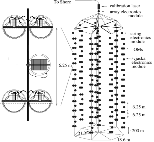
Figure 1: A schematic view of NT200. The expansion left-hand shows 2 pairs of optical modules (“svjaska”) with the svjaska electronics module, which houses part of the readout and control electronics.

An umbrella-like frame carries 8 strings, each with 24 pairwise arranged OMs. All OMs face downward, with the exception of the second and eleventh pairs on each string which face upward. Three underwater electrical cables connect the detector with the shore station. Each OM contains a 37-cm diameter QUASAR - photo multiplier (PM), which has been developed specially for our project [5]. The PMs record the Cherenkov light produced by charged particles in water. The two PMs of a pair are switched in coincidence in order to suppress background from bioluminescence and PM noise. A pair of OMs defines a channel. The light arrival time assigned to a channel is the response time of the OM with the earliest hit. The amplitude assigned to a channel is that recorded by one pre-selected PM of the two PMs in a pair. For those channels for which one of the two OMs failed and the single PM noise rates of the remaining OM are not too high (smaller than the average noise rate of 100 kHz), that OM is operated in single mode (1PM/channel), with a threshold slightly higher than the typical 0.3 photo electrons.

A trigger is formed by the requirement of $\geq N$ hits (with hit referring to a channel) within 500 ns. $N$ is typically set to 3 or 4. For these events, amplitude and time of all fired channels are digitized and sent to shore.

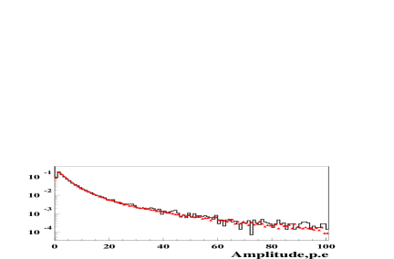
Figure 2: Left panel: the normalized amplitude distribution for channel 2 (points – experiment, histogram – atmospheric muon simulation). Right panel: the normalized time difference of channel 42 and channel 43. Histogram - experiment, dashed histogram - expectation from atmospheric muons.

Two nitrogen lasers are used for calibration of the detector. The first one (fiber laser) is mounted just above the array. Its light is guided via optical fibers of equal length to each OM pair. The fiber laser provides the OMs with simultaneous light signals in order to determine the offset for each channel. The second laser (water laser) is arranged 20 m below the array. Its light propagates through the water. This laser serves to monitor the water quality, in addition to dedicated environmental devices located along a separate string. In the context of this analysis, however, its main purpose is to simulate high energy particle cascades outside the geometrical volume of NT200. The maximum light intensity of the water laser ($\sim$10¹¹ photons/pulse) roughly corresponds to the Cherenkov radiation emitted by high-energy cascades with $E_{cas}\approx$1 PeV. A full cycle of detector calibration running both lasers over a wide range of intensities is repeated every third day.

Figure 2 demonstrates the level to which basic features of the detector are understood and can be reproduced by Monte-Carlo (MC) simulations. We have used atmospheric muons as a high statistics standard calibration signal. The figure shows distributions of recorded amplitudes and light arrival time differences compared to MC-simulation. The experimental data are in good agreement with simulation (see also [2]).

Lake Baikal deep water is characterized by an absorption length of $L_{abs}$(480 nm)=20$\div$24 m, a scattering length of $L_{s}=$30$\div$70 m and a strongly anisotropic scattering function $f(\theta)$ with a mean cosine of the scattering angle $\overline{\cos}(\theta)=0.85\div 0.9$.

3 The analysis method

3.1 Search strategy

The BAIKAL survey for high energy neutrinos searches for bright cascades produced at the neutrino interaction vertex in a large volume around and below the neutrino telescope (see fig. 3). Lack of significant light scattering allows to monitor a volume exceeding the geometrical volume by more than an order of magnitude. This results in sensitivities for high energy cascade detection which are close to those of the much larger AMANDA detector [6]. The main background source to this analysis are atmospheric muons, with a flux 10⁶ times higher than that of atmospheric neutrinos.

We select events with high multiplicity of hit channels $N_{\mbox{\small hit}}$, corresponding to bright cascades. The main remaining background to isolated cascades from neutrino interactions are then cascades from bremsstrahlung along energetic downward muons. To separate high-energy neutrino events from background events a cut on the variable $t_{\mbox{\footnotesize min}}=\mbox{\footnotesize min}(t_{i}-t_{j})$ (with $i<j$) is applied.

Figure 3: Detection principle for neutrino induced cascades with NT200.

Here, $t_{i},\,t_{j}$ are the arrival times at channels $i,j$ on each string (the numbering of channels is from top to bottom along strings), the minimum over all strings is calculated. Positive and negative values of $t_{\mbox{\footnotesize min}}$ correspond to upward and downward propagation of light, respectively. We require

$$t_{\mbox{\footnotesize min}}>-10\,\,\mbox{ns}.$$ (4)

This cut accepts only time patterns corresponding to upward traveling light signals. It rejects most events from brems-cascades produced by downward going muons since the majority of muons is close to the vertical; they would cross the detector or pass nearby and generate a downward time pattern. Only few muons with large zenith angles may escape this cut and illuminate the array by their own Cherenkov radiation or that from bright cascades from below.

The energy spectrum of neutrinos from galactic and cosmological sources or from the decay of topological defects is expected to have a significantly flatter shape than the spectrum of atmospheric muons. This is reflected by different $N_{\mbox{\small hit}}$ distributions. In fig. 4 we show $N_{\mbox{\small hit}}$ distributions of simulated events which survive cut (4) and would be induced by electron neutrinos with fluxes of shape $\sim E^{-\gamma}$, with $\gamma$=1.5, 2 and 2.5 (normalized to each other, simulations is for 80 operating channels). Also shown is the $N_{\mbox{\small hit}}$ distribution of background events induced by atmospheric muons (normalized arbitrarily to neutrino events). This distribution is much steeper, so that an extraterrestrial neutrino signal would appear as an excess of events with large $N_{\mbox{\small hit}}$ above the background of atmospheric muons.

Figure 4: The normalized hit multiplicity distributions of events from $\nu_{e}$ fluxes after selection criterion (4). Solid, dashed and dotted histograms correspond to $\gamma$=1.5, 2, 2.5, respectively. Also shown is the $N_{\mbox{\small hit}}$ distribution of background events from atmospheric muons (thick line).

3.2 Laser calibration

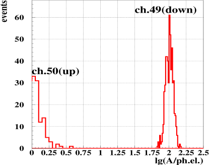
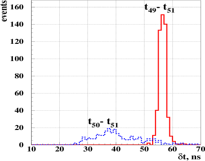
Figure 5: Laser calibration: left panel - the amplitude distributions of channels directed downward (channel 49) and upward (channel 50). Right panel: time difference distribution $\delta t$ for pairs of channels facing both downward (49,51) and upward (50)/downward (51), respectively.

As mentioned above, a central purpose of the water laser is to investigate the response of NT200 to bright light sources below the detector. The water laser is mounted on the central string about 20 m below the bottom OMs of NT200. An attenuator allows to operate the device with five gradually decreasing light pulse intensities. In the most powerful mode, about 10¹¹ photons/pulse are emitted isotropically. Figure 5 (left panel) shows the amplitudes on channel 49 (turned downward) and channel 50 (turned upward) induced by these pulses. The distances between the water laser and channels 49 and 50 (both on central string and above water laser) are 88.8 m and 81.3 m, respectively. In contrast to channel 49, which faces the light source, channel 50 is directed in the opposite direction. Therefore it is almost blind to direct light and detects mostly scattered photons. Due to the low scattering coefficient of Baikal water, the signals in channel 50 are about 70 times lower than in channel 49.

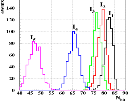
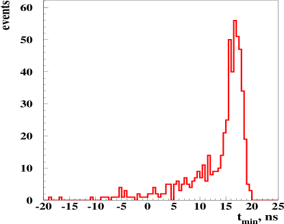
Figure 6: Left panel: the hit channels multiplicity of events induced by laser pulses with five different intensities for. Right panel: the $t_{\mbox{\footnotesize min}}$ distribution for laser events.

Figure 5 (right panel) shows the difference $\delta t$ of laser light arrival times on channel 49 (channel 50) and channel 51. Like channel 49, channel 51 is turned downward. It is located 12.5 m below channel 49. The r.m.s. of $\delta t=(t_{49}-t_{51})$, i.e. for the two downward looking channels, is about 1.4 ns. It is not affected by light scattering in water and entirely due to experimental time resolution. The r.m.s. of $\delta t=(t_{50}-t_{51})$ is about 8.4 ns. This large value is caused by the dispersion of photon arrival times on channel 50 due to light scattering. To reach maximum background suppression in the cascade search by application of strict arrival time cuts, we exclude upward looking channels from the analysis.

The distributions of the variables $N_{\mbox{\small hit}}$ and $t_{\mbox{\footnotesize min}}$, which are used for the selection of neutrino induced events, are shown in fig. 6. Distributions on the left panel correspond to the five laser intensities - 1.2$\times$10¹¹, 2.2$\times$10¹⁰, 4.7$\times$10⁹, 1.0$\times$10⁹ and 2.5$\times$10⁸ photons/pulse - which approximately correspond to cascade energies 1200, 220, 47, 10 and 2.5 TeV, respectively. The $t_{\mbox{\footnotesize min}}$ distribution on the right panel corresponds to the most powerful laser intensity mode. In agreement with above discussion of the upward moving light selection criteria (4) we found for nearly all laser events $t_{\mbox{\footnotesize min}}>-$10 ns.

The high transparency and the low scattering of Baikal water allow the reconstruction of coordinates and intensity of bright light flashes. The laser experiment allowed to verify the reconstruction procedure of shower position and intensity. We found a vertical laser coordinate precision of $\sim$1 m and relative intensity precision of $\sim$10 % [7].

3.3 High-energy neutrino simulation

The number of expected events $N_{\nu_{i}}$ during observation time T is:

$$N_{\nu_{i}}=T\int d\vec{\Omega}\int dE_{h}V_{eff}(\vec{\Omega},E_{sh})\times$$

$$\sum_{k}\int N_{A}\rho_{H_{2}O}\frac{d\sigma_{\nu k}}{dE_{h}}\Phi_{\nu_{i}}(\vec{\Omega},E_{\nu},X)dE_{\nu}$$ (5)

$$X(\vec{\Omega})=\int_{0}^{L}\rho_{earth}(l)dl,$$

where $\Phi_{\nu_{i}}(\vec{\Omega},E_{\nu},X)$ is the flux of high energy neutrinos with energy $E_{\nu}$ in the vicinity of the detector, $\vec{\Omega}$ - the neutrino direction, $X(\vec{\Omega})$ - the thickness of matter encountered by the neutrino on its passage through the Earth, $E_{\mbox{\footnotesize h}}$ - the energy transferred to the hadron, $E_{\mbox{\footnotesize sh}}$ - total energy of secondary showers, $V_{\mbox{\footnotesize eff}}(\vec{\Omega},E_{\mbox{\footnotesize sh}})$ - the detection volume. The index $\nu_{i}$ indicates the neutrino type ($\nu_{i}=\nu_{e},\bar{\nu_{e}},\nu_{\mu},\bar{\nu_{\mu}},\nu_{\tau},\bar{\nu_{\tau}}$) and $k=$1,2 corresponds to CC- and NC-interactions respectively. $N_{A}$ is the Avogadro number and $\rho_{H_{2}O}$ the water density.

For $\nu_{e}$ and $\nu_{\mu}$, the flux $\Phi_{\nu}$ satisfies the following transport equation:

$$\frac{d\Phi_{\nu}(E_{\nu})}{dX}=-N_{A}\sigma_{tot}\Phi_{\nu}(E_{\nu})+$$

$$N_{A}\int_{E_{\nu}}^{\propto}dE^{\prime}_{\nu}\Phi_{\nu}(E^{\prime}_{\nu})\frac{d\sigma^{NC}}{dE_{\nu}}(E^{\prime}_{\nu},E_{\nu})$$ (6)

where $\sigma_{tot}=\sigma_{CC}+\sigma_{NC}$.

For $\nu_{\tau}$, the tau neutrino and tau lepton fluxes satisfy the equations:

$$\frac{d\Phi_{\nu_{\tau}}(E_{\nu_{\tau}})}{dX}=-N_{A}\sigma_{tot}\Phi_{\nu_{\tau}}(E_{\nu_{\tau}})+$$

$$N_{A}\int_{E_{\nu_{\tau}}}^{\propto}dE^{\prime}_{\nu_{\tau}}\Phi_{\nu_{\tau}}(E^{\prime}_{\nu_{\tau}})\frac{d\sigma^{NC}}{dE_{\nu_{\tau}}}(E^{\prime}_{\nu_{\tau}},E_{\nu_{\tau}})$$

$$+\int_{E_{\nu_{\tau}}}^{\propto}dE_{\tau}\frac{\Phi_{\tau}(E_{\tau})}{\lambda^{dec}_{\tau}}\frac{dn}{dE_{\nu_{\tau}}}(E_{\tau},E_{\nu_{\tau}})$$ (7)

$$\frac{d\Phi_{\tau}(E_{\tau})}{dX}=-\frac{\Phi_{\tau}(E_{\tau})}{\lambda^{dec}_{\tau}(E_{\tau})}+$$

$$N_{A}\int_{E_{\tau}}^{\propto}dE_{\nu_{\tau}}\Phi(E_{\nu_{\tau}})\frac{d\sigma^{CC}}{dE_{\tau}}(E_{\nu_{\tau}},E_{\tau})$$

where $\lambda^{dec}_{\tau}=\gamma c\tau_{\tau}\rho$ is the decay length of the $\tau$-lepton, $dn/dE_{\nu_{\tau}}$ - $\nu_{\tau}$ production probability. The transport equation for the $\tau$-lepton is valid under the assumption that $\lambda^{dec}_{\tau}/\lambda_{\tau}<<1$, where $\lambda_{\tau}$ - the interaction length of $\tau$ propagation through the medium. This assumption is valid for energies $E_{\tau}<$10⁸ GeV.

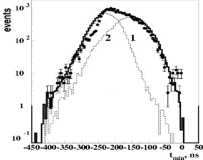
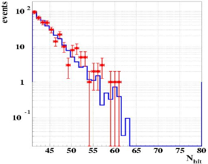
Figure 7: Left panel: the $t_{\mbox{\footnotesize min}}$ distributions for experiment (dots) and atmospheric muon simulation (bold histogram) for $N_{\mbox{\small hit}}>$40. Histograms 1 and 2 correspond to atmospheric muon simulation with $\cos\theta>0.8$ and $\cos\theta<0.8$, respectively. Right panel: the $N_{\mbox{\small hit}}$ distributions for experiment (dots) and atmospheric muon simulation (histogram) with $t_{\mbox{\footnotesize min}}>$-100 ns.

A MC-code is used to solve equations (6) - (7), with the boundary conditions for neutrino fluxes $\Phi_{\nu_{i}}(E,0)=A_{\nu_{i}}f_{\nu_{i}}(E)$, where $f_{\nu_{i}}(E)$ is a diffuse AGN-like flux or other predicted UHE neutrino fluxes, and a $A_{\nu_{i}}$ a normalization coefficient. For tau leptons $\Phi_{\tau}(E,0)=0$. For neutrino interactions and tau-neutrino regeneration we used cross-sections from [8, 9]. The neutrinos are propagated through the Earth assuming the density profile of the Preliminary Reference Earth Model [10]. Although a flavor ratio of $\nu_{e}:\nu_{\mu}:\nu_{\tau}\approx$1:2:0 is predicted for generic neutrino fluxes at cosmic sources, equal fractions of all three neutrino flavors are expected at Earth because of neutrino oscillations. Throughout this paper we assumed a neutrino flavor ratio at Earth of $\nu_{e}:\nu_{\mu}:\nu_{\tau}=$1:1:1 and the same shape of energy spectra $f(E_{\nu})$ for all neutrino flavors, as well as a flux ratio for neutrino and antinutrino of $\nu/\bar{\nu}=$1.

The detector response to Cherenkov radiation of high energy cascades was simulated taking into account the effects of absorption and scattering of light as well as light velocity dispersion in water [11, 12, 13]. We also implemented the longitudinal development of cascades. For electron cascades with $E_{\mbox{\footnotesize sh}}>$2$\times$10⁷ GeV and for hadronic cascades with $E_{\mbox{\footnotesize sh}}>$10⁹ GeV, the increase in cascade length due to the LPM effect [14] was approximated as $E^{1/3}$ according to Ref. [15].

3.4 Atmospheric muon simulation

Downward going atmospheric muons are the most important source of background. The simulation chain of these muons starts with cosmic ray air shower generation using the CORSIKA program [16] with the QGSJET [17] interaction model and the primary composition and spectral slopes for individual elements taken from [18]. Atmospheric muons are propagated through the water using the MUM program [19]. During passage through the detection volume the detector response to Cherenkov light from all muon energy loss processes is simulated.

For illustration of the consistency of experimental data with simulation we present in fig. 7 (left panel) the $t_{\mbox{\footnotesize min}}$ distributions for simulated background events (histograms), as well as for experimental events with a hit multiplicity $N_{\mbox{\small hit}}>40$ taken during 41.8 live days in 1999. Curves 1 and 2 correspond to atmospheric muons with zenith angles $\cos\theta>0.8$ and $\cos\theta<0.8$, respectively. We find good agreement for all $t_{\mbox{\footnotesize min}}$ values, with a small deficit only for vertical downward going muons in the interval -300, -230 ns (i.e. far-off the cut value -10 ns). This deficit is due to the difficulty to precisely determine the low OM detection efficiency of downward looking OMs for straight backward light illumination by vertical atmospheric muons. Figure 7 (right panel) shows the $N_{\mbox{\small hit}}$ distribution of events with $t_{\mbox{\footnotesize min}}>$-100 ns as well as background simulation (histogram). We conclude that experimental $t_{\mbox{\footnotesize min}}$ and $N_{\mbox{\small hit}}$ distributions are consistent with distributions expected for atmospheric muons.

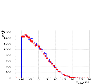
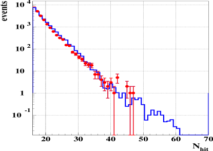
Figure 8: Left panel: the $t_{\mbox{\footnotesize min}}$ distribution of experimental events (dots) which survive cut (4) as well as the expected distribution of simulated background events (histogram). Right panel: the $N_{\mbox{\small hit}}$ distribution of experimental events (dots) as well as the background prediction (histogram) after cut (4).

4 Data selection and analysis

Within the 1038 days of the detector live time between April 1998 and February 2003, $3.45\times 10^{8}$ events with $N_{\mbox{\small hit}}\geq 4$ have been recorded. For this analysis we used 22597 events with hit channel multiplicity $N_{\mbox{\small hit}}>$15 which obey the condition (4). For these events upward looking channels as well as channels which are operated in the 1-PM/channel mode (see section 2) have been excluded from the following analysis.

Table 1: NT200 effective configurations.

Conf.	$\bar{N}_{\mbox{\footnotesize op}}$	$T$	$N_{\mbox{\footnotesize ev}}$	$N_{\mbox{\footnotesize hit}}^{\mbox{\footnotesize max}}$
		(days)
1	71	316	12146	47
2	59	612	9473	42
3	46	110	978	32

During the 1038 days NT200 took data in various configurations, which have evolved due to groups of OMs failing. Neglecting few-OM differences, the data can be grouped according to three basic configurations. The average number of working channels $\bar{N}_{\mbox{op}}$, the data taking time $T$, the number of detected events $N_{\mbox{ev}}$, as well as the largest multiplicity of hit channels for detected events $N_{\mbox{\small hit}}^{\mbox{\small max}}$ are shown in Table 1.

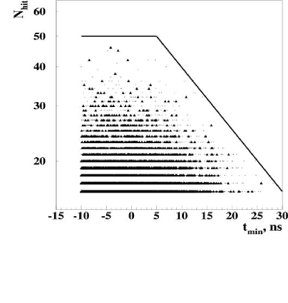
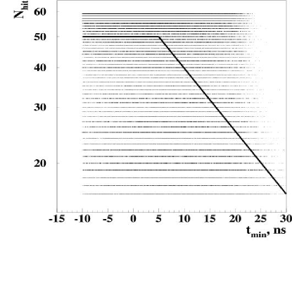
Figure 9: Left panel: distributions of experimental (triangles) and expected background (dots) events in the ($t_{\mbox{\footnotesize min}},N_{\mbox{\small hit}}$)-plane. Right panel: same distribution for events expected from high energy cascades. Results are shown for configuration 1 (Table 1). The line shows cut condition (see Table 2).

Table 2: Cut conditions in the ($t{\mbox{\footnotesize min}},N_{\mbox{\small hit}}$)-plane used for the selection of neutrino induced events ($t{\mbox{\footnotesize min}}$ in ns).

Conf. 1	-10$<t_{\mbox{\footnotesize min}}\leq$5	5 $<t_{\mbox{\footnotesize min}}\leq$30	$t_{\mbox{\footnotesize min}}>$30
	$N_{\mbox{\small hit}}\geq$ 50	$N_{\mbox{\small hit}}\geq$ 10${}^{(1.8-0.02t_{min})}$	$N_{\mbox{\small hit}}\geq$ 16
Conf. 2	-10 $<t_{\mbox{\footnotesize min}}\leq$10	10$<t_{\mbox{\footnotesize min}}\leq$30	$t_{\mbox{\footnotesize min}}>$30
	$N_{\mbox{\small hit}}\geq$ 44	$N_{\mbox{\small hit}}\geq$ 10${}^{(1.865-0.0223t_{min})}$	$N_{\mbox{\small hit}}\geq$ 16
Conf. 3	-10 $<t_{\mbox{\footnotesize min}}\leq$10	10 $<t_{\mbox{\footnotesize min}}\leq$30	$t_{\mbox{\footnotesize min}}>$30
	$N_{\mbox{\small hit}}\geq$ 33	$N_{\mbox{\small hit}}\geq$ 42-0.9$t_{\mbox{\footnotesize min}}$	$N_{\mbox{\small hit}}\geq$ 16

Figure 8 shows the $t_{\mbox{\footnotesize min}}$ and $N_{\mbox{\small hit}}$ distributions for experiment (dots) and background simulation (histograms). We conclude that after application cut (4) data are consistent with simulated background for both $t_{\mbox{\footnotesize min}}$ and $N_{\mbox{\small hit}}$ distributions. No statistically significant excess above the background from atmospheric muons has been observed.

To maximize the sensitivity to a neutrino signal we introduce a cut in the ($t_{\mbox{\footnotesize min}},N_{\mbox{\small hit}}$) phase space. Figure 9 (left panel) shows the population of the ($t_{\mbox{\footnotesize min}},N_{\mbox{\small hit}}$) phase space for experimental events (triangles) as well as for background simulation (dots). The distribution for neutrino induced events (dots) is shown in the right panel of fig. 9 (for spectral index $\gamma=-$2). We note that background events populate the lower-left part of the plot, in contrast to signal events. The bounds which fence the ($t_{\mbox{\footnotesize min}},N_{\mbox{\small hit}}$) area which we assigned to background are listed in Table 2 for the three NT200 configurations.

With no experimental events outside the area populated by background events in the ($t_{\mbox{\footnotesize min}},N_{\mbox{\small hit}}$) phase space we can derive upper limits on the fluxes of high energy neutrinos as predicted by different models of neutrino sources.

The neutrino detection energy range of NT200 which contains, for instance, 90% of expected events, depends on the energy shape of the neutrino flux. Figure 10 shows the fractions of expected events induced by diffuse neutrino fluxes following an $E^{-\gamma}$ shape with spectral indices $\gamma$=1, 1.5, 2, 2.5 and 3.7, for energies ranges 10 TeV$<E<E_{\nu}$. The effective detection range is shifting towards higher energies with decreasing $\gamma$. Table 3 shows the energy ranges for effective detection of neutrino fluxes with different $\gamma$, as well as the median values of the energy distributions.

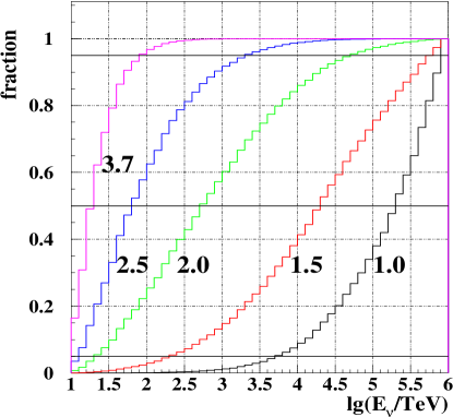
Figure 10: The fraction of expected events induced by diffuse $\nu_{e}$ fluxes with spectral indices $\gamma$=1, 1.5, 2, 2.5 and 3.7 within energy range 10 TeV$<E<E_{\nu}$.

Table 3: Detection energy range and median energy for different spectra.

$\gamma$	$\Delta E$, TeV	$E_{\mbox{med}}$, TeV
1.0	5$\times$103 - 7$\times$105	2.2$\times$105
1.5	2$\times$102 - 5.6$\times$105	2.0$\times$104
2.0	22 - 5.0$\times$104	5.6$\times$102
2.5	14 - 2.0$\times$103	63
3.7	10 - 89	20

With increasing energy, neutrinos are stronger absorbed when propagating through the Earth, and upward going fluxes are suppressed. Our search strategy accepts neutrinos from all directions. With increasing neutrino energy the angular distributions are shifted towards smaller zenith angles. Zenith angle ranges $\Delta\theta$ which contain 90% of expected events induced by an $E^{-2}$ neutrino flux are 75^o - 150^o and 40^o - 90^o for energy ranges 10 TeV - 100 TeV and 10⁵ - 10⁶ TeV, respectively.

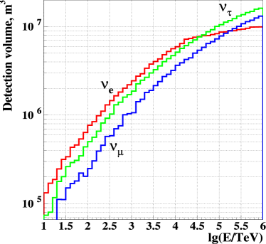
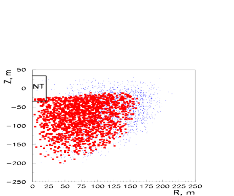
Figure 11: Left panel: energy dependence of detection volumes. Right panel: coordinates of $\nu_{e}$ interaction vertices for events which fulfill cut (4) (dots) and all final cuts for neutrino event selection (rectangles), respectively. The ordinate gives the vertical position, the abscissa the radial distance, with (z=0, R=0) corresponding to the center of NT200. The small rectangle marks the geometrical volume of NT200.

The detection volumes V${}_{\mbox{\footnotesize eff}}$ for all three neutrino flavors after all cuts were calculated as a function of neutrino energy and zenith angle $\theta$. The energy dependence of the detection volumes, averaged over all neutrino arrival directions, are shown in fig. 11 (left panel). The value of $V_{\mbox{\footnotesize eff}}$ rises from $\sim$10⁵ m³ for 10 TeV up to (4-6)$\times$10⁶ m³ for $10^{4}$ TeV and significantly exceeds the geometrical volume $V_{\mbox{\footnotesize g}}\approx$ 10⁵ m³ of NT200. This is due to the low light scattering and the nearly not distorted light fronts from Cherenkov waves originating far outside the geometrical volume. In the case of $\nu_{e}$ detection, the volume saturates for $E_{\nu_{e}}>$10⁴ TeV because of the LPM effect. Figure 11 (right panel) illustrates the difference between $V_{\mbox{\footnotesize eff}}$ and $V_{\mbox{\footnotesize g}}$. Shown here are the coordinates of neutrino interaction vertices for events which survive cuts (4) (dots) and all cuts (rectangles), assuming an $E^{-2}$ spectrum.

Systematic uncertainties in the optical properties of water, the absolute detector sensitivity and the neutrino cross sections at high energies influence the number of expected signal events. The uncertainty of 10% in absorption length results in 20% uncertainty in the number of expected events. The uncertainty of 14% in the sensitivity of OMs results in 10% uncertainty in the number of expected events. Below 10¹⁶ eV, all standard sets of parton distributions yield very similar cross sections. Above this energy, the cross sections are sensitive to assumptions made about the behavior for $x\rightarrow 0$. The uncertainties of cross sections are less than 10% below 10¹⁸ eV [8, 20, 21] and result in uncertainties of 8% in the number of expected events. Treating these errors as independent and adding them quadratically, the signal uncertainty becomes 24%.

5 Limits on the high energy neutrino fluxes

Table 4: Expected number of events $N_{\mbox{\footnotesize model}}$ and model rejection factors for models of astrophysical neutrino sources. The assumed upper limit on the number of signal events with all uncertainties incorporated is $n_{90\%}=2.5$

	BAIKAL					AMANDA [6, 24]
Model	$\nu_{e}$	$\nu_{\mu}$	$\nu_{\tau}$	$\nu_{e}+\nu_{\mu}+\nu_{\tau}$	$n_{90\%}/N_{\mbox{\footnotesize model}}$	$n_{90\%}/N_{\mbox{\footnotesize model}}$
10${}^{-6}\times E^{-2}$	1.33	0.63	1.12	3.08	0.81	0.86
SS Quasar [25]	4.16	2.13	3.71	10.00	0.25	0.21
SP u [26]	17.93	7.82	14.43	40.18	0.062	0.054
SP l [26]	3.14	1.24	2.37	6.75	0.37	0.28
P $p\gamma$ [27]	0.81	0.53	0.85	2.19	1.14	1.99
M $pp+p\gamma$ [28]	0.29	0.22	0.35	0.86	2.86	1.19
MPR [29]	0.25	0.14	0.24	0.63	4.0	4.41
SeSi [30]	0.47	0.26	0.44	1.18	2.12	-

Since no events have been observed which pass the final cuts (see Table 2), upper limits on the diffuse flux of extraterrestrial neutrinos are calculated. For a 90% confidence level an upper limit on the number of signal events of $n_{90\%}=$2.5 is obtained according to Conrad et al. [22] with the unified Feldman-Cousins ordering [23]. We assume an uncertainty in signal detection of 24% and a background of zero events (which leads to a conservative estimation of $n_{90\%}$ according to the Feldman-Cousins approach).

The expected number of signal events $N_{\nu_{i}}$ for any assumed flux $\Phi_{\nu_{i}}(E)$ of neutrinos of flavor $i$, is given by expression (5). A model of astrophysical neutrino sources, for which the total number of expected events, $N_{\mbox{\footnotesize model}}$, is large than $n_{90\%}$, is ruled out at 90% CL. $N_{\mbox{\footnotesize model}}$ is given as $N_{\mbox{\footnotesize model}}=\sum N_{\nu_{i}}$. Table 4 represents event rates and model rejection factors (MRF) $n_{90\%}/N_{\mbox{\footnotesize model}}$ for models of astrophysical neutrino sources obtained from our search. Recently, similar results have been presented by the AMANDA collaboration [6, 24], model rejection factors are shown in Table 4.

The models by Stecker and Salamon [25] labeled “SS Q”, as well as the models by Szabo and Protheroe [26] “SP u” and “SP l” represent models for neutrino production in the central region of Active Galactic Nuclei. As can be seen from Table 4, these models are ruled out with $n_{90\%}/N_{\mbox{\footnotesize model}}\approx$ 0.06 - 0.4. Further shown are models for neutrino production in AGN jets: calculations by Protheroe [27] and by Mannheim [28], which include neutrino production through $pp$ and $p\gamma$ collisions (models “P $p\gamma$” and “M $pp+p\gamma$”, respectively), as well as an evaluation of the maximum flux due to a superposition of possible extragalactic sources by Mannheim, Protheroe and Rachen [29] (model “MPR”) and a prediction for the diffuse flux from blazars by Semikoz and Sigl [30] “SeSi”. The latter models for blazars are currently not excluded.

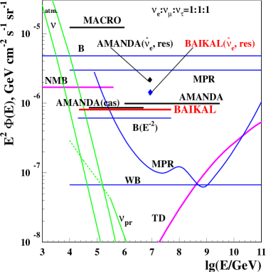
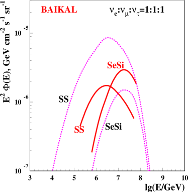
Figure 12: Left panel: all-flavor neutrino flux predictions in different models of neutrino sources compared to experimental upper limits to $E^{-2}$ fluxes obtained by this analysis and other experiments (see text). Right panel: Baikal experimental limits compared to two model predictions. Dotted curves: predictions from model SS [25] and SeSi [30]. Full curves: upper limits to spectra of the same shape. Model SS is excluded (MRF=0.25), model SeSi is not (MRF=2.12).

For an $E^{-2}$ behaviour of the neutrino spectrum and a flavor ratio $\nu_{e}:\nu_{\mu}:\nu_{\tau}=1:1:1$, the 90% C.L. upper limit on the neutrino flux of all flavors obtained with the Baikal neutrino telescope NT200 (1038 days) is:

$$E^{2}\Phi<8.1\times 10^{-7}\mbox{cm}^{-2}\mbox{s}^{-1}\mbox{sr}^{-1}\mbox{GeV}.$$

(8)

For the resonant process

$$\bar{\nu_{e}}+e^{-}\rightarrow W^{-}\rightarrow\mbox{anything},$$ (9)

with the resonant neutrino energy $E_{0}=M^{2}_{w}/2m_{e}=6.3\times 10^{6}\,$GeV and a cross section $5.02\times 10^{-31}$cm², the event number is given by:

$$N_{\bar{\nu_{e}}}=T\int d\Omega\int dEV_{eff}\int\limits_{E^{-}}^{E^{+}}dE_{\nu}\times$$

$$\times\Phi_{\bar{\nu_{e}}}(E_{\nu})\frac{10}{18}N_{A}\rho_{H_{2}O}\frac{d\sigma_{\bar{\nu_{e}},e}}{dE},$$ (10)

where $E^{\pm}=(M_{w}\pm 2\Gamma_{w})^{2}/2m_{e}$ and $M_{w}=$80.22 GeV, $\Gamma_{w}=$2.08 GeV.

Assuming an upper limit on the number of signal events $n_{90\%}=$2.5, the model-independent limit on $\bar{\nu_{e}}$ at the W - resonance energy is:

$$\Phi_{\bar{\nu_{e}}}<3.3\times 10^{-20}\mbox{cm}^{-2}\mbox{s}^{-1}\mbox{sr}^{-1}\mbox{GeV}^{-1}.$$

(11)

Figure 12 (left panel) shows our upper limit on the all flavor $E^{-2}$ diffuse flux (8) as well as the model independent limit on the resonant $\bar{\nu}_{e}$ flux (diamond) (11). Also shown are the limits obtained by AMANDA and MACRO [6, 24, 31], theoretical bounds obtained by Berezinsky (model independent (B) and for an $E^{-2}$ shape of the neutrino spectrum (B($E^{-2}$)) [32], by Waxman and Bahcall (WB) [33], by Mannheim et al.(MPR) [29], predictions for neutrino fluxes from topological defects (TD) [30], prediction on diffuse flux from AGNs according to Nellen et al. (NMB) [34], as well as the atmospheric conventional neutrino fluxes [35] from horizontal and vertical directions ( ($\nu$) upper and lower curves, respectively) and atmospheric prompt neutrino fluxes ($\nu_{pr}$) obtained by Volkova et al. [36]. The right panel of fig. 12 shows our upper limits (solid curves) on diffuse fluxes from AGNs shaped according to the model of Stecker and Salamon (SS) [25] and of Semikoz and Sigl (SeSi) [30], according to Table 4.

The diffuse neutrino flux is assumed to be composed of contributions from cosmological sources with different luminosity and energy spectra. To benchmark the energy dependence of our limit without referring to a special model, we show in Fig.13 the upper limits derived for $E^{-1}$ spectra with variable, sharp cutoff. The parts of the spectra drawn with thick lines cover the energy ranges containing 90% of expected events. Also shown is a curve connecting the points which correspond to the median energies of recorded events. This curve represents the upper limit on a diffuse flux formed by superposition of the benchmark spectra. Also shown (horizontal line) is the upper limit on an $E^{-2}$ spectrum, as given in (8) above.

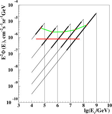
Figure 13: Upper limits on $E^{-1}$ benchmark spectra with variable cutoff. Thick lines cover the energy ranges containing 90% of expected events. Points at the median energies are connected by the thick curve. Also shown is the upper limit on $E^{-2}$ spectrum.

6 Conclusion

The neutrino telescope NT200 in Lake Baikal is taking data since April 1998. Due to high water transparency and low light scattering, the detection volume of NT200 for high energy $\nu_{e}$, $\nu_{\mu}$ and $\nu_{\tau}$ events is several megatons and exceeds the geometrical volume by a factor of about 50 for highest energies. This results in a high sensitivity to diffuse neutrino fluxes from extraterrestrial sources – more than an order of magnitude better than that of underground searches and similar to the published limits of AMANDA, the other operating large neutrino telescope. The upper limit obtained for a diffuse ($\nu_{e}+\nu_{\mu}+\nu_{\tau}$) flux with $E^{-2}$ shape is $E^{2}\Phi=8.1\times 10^{-7}$cm^-2s^-1sr^-1GeV. With $3.3\times 10^{-20}$cm^-2s^-1sr^-1GeV^-1, the limit on a $\bar{\nu_{e}}$ flux at the resonant energy 6.3$\times$10⁶GeV is presently the most stringent.

To extend the search for diffuse extraterrestrial neutrinos with higher sensitivity, NT200 was significantly upgraded. [37]. In March/April 2005 we fenced a large part of the search volume (see Fig.12, right) with three sparsely instrumented strings. The three-year sensitivity of this enlarged detector NT200$+$ on the neutrino flux of all flavors, with about 5 Mton enclosed volume, is approximately $2\times 10^{-7}$cm^-2s^-1sr^-1GeV for $E>$10² TeV, i.e. three-four times better than that of NT200. NT200$+$ will search for neutrinos from AGNs, GRBs and other extraterrestrial sources, neutrinos from cosmic ray interactions in the Galaxy as well as high energy atmospheric muons with $E_{\mu}>10$ TeV.

7 Acknowledgments

This work was supported by the Russian Ministry of Education and Science, the German Ministry of Education and Research and the Russian Fund of Basic Research (grants 05-02-17476 and 04-02-17289), and by the Grant of President of Russia NSh-1828.2003.2.

References

- [1] V.A.Balkanov et al. [BAIKAL Collaboration], Astropart. Phys., 14 (2000) 61.
- [2] I.A. Belolaptikov et al. [BAIKAL Collaboration], Astropart. Phys. 7 (1997) 263.
- [3] V.A.Balkanov et al. [BAIKAL Collaboration], Astropart. Phys. 12 (1999) 75.
- [4] V.A. Balkanov et al. [BAIKAL Collaboration], Nucl. Phys. (Proc. Suppl.) B91 (2001) 438.
- [5] R.I.Bagduev et al. Nucl. Instr. Meth. A420 (1999) 138.
- [6] M. Ackermann et al., Astropart Phys. 22 (2004) 127.
- [7] B.A. Shaibonov, Diploma thesis, Moscow Phys. Eng. Inst., (2003) Moscow (in russian).
- [8] R. Gandhi et al., Astropart. Phys. 5 (1996) 81; R. Gandhi et al., Phys. Rev. D58 (1998) 093009.
- [9] P. Lipari, Astropart. Phys. 1 (1993) 195.
- [10] A.M. Dziewonski, D.L. Anderson, Phys. Earth Planet. Interiors 25 (1981) 297.
- [11] L.A.Kuzmichev. NIM, A482 (2001) 304.
- [12] Zh.-A.M. Dzhilkibaev, and B.A. Shai- bonov, Preprint INR-1073/2002 (2002) (in russian).
- [13] Zh.-A. Dzhilkibaev, A. Gazizov, and Ch. Spiering, Proc. of the workshop on Technical Aspects of a Very Large Volume Neutrino Telescope in the Mediterranean, ed. by E. de Wolf, Amsterdam (2003) 99.
- [14] A. Migdal, Phys. Rev., 103 N6 (1956) 1811.
- [15] J. Alvarez-Muniz, E. Zas, Phys. Lett. B411 (1997) 218.
- [16] J. Capdevielle et. al., KfK Report 4998, Kernforschungszentrum, Karlsruhe (1992).
- [17] N.N. Kalmykov, S.S. Ostapchenko and A.I. Pavlov, Nucl. Phys. (Proc. Suppl.) B52 (1997) 17.
- [18] B. Wiebel-Smooth, P. Biermann and Landolt-Bornstein, Cosmic Rays, v. 6/3c, Springer Verlag (1999) 37-90.
- [19] E.V. Bugaev et al., Phys. Rev. D64 (2001) 074015.
- [20] M. Gluck, S. Kretzer and E. Reya, Inst. fur Physik, Univ. Dortmund, DO-th 98/20 (1998) 1-16; arXiv:astro-ph/9809273.
- [21] J. Kwiecinski, A. Martin and A.M. Stasto, Univ. of Durham, DTP-98-98 (1998) 1-28; arXiv:astro-ph/9812262.
- [22] J. Conrad et al., Phys. Rev. D67 (2003) 012002.
- [23] G.J. Feldman and R.D. Cousins, Phys. ReV. D57 (1998) 3873.
- [24] M. Ackermann et al., Astropart. Phys. 22 (2005) 339.
- [25] F. Stecker and M. Salamon, Space Sci. Rev. 75 (1996) 341.
- [26] A. Szabo and R. Protheroe, Proc. High Energy Neutrino Astrophy- sics, ed. V.J. Stenger et al., Honolulu, Hawaii (1992).
- [27] R.J. Protheroe, arXiv:astro-ph /9612213.
- [28] K. Mannheim, Astropart. Phys. 3 (1995) 295.
- [29] K. Mannheim, R.J. Protheroe and J.P. Rachen, Phys. Rev. D63 (2001) 023003.
- [30] D. Semikoz and G. Sigl, arXiv:hep-ph/0309328.
- [31] M. Ambrosio et al., Nucl. Phys. (Proc. Suppl.) B110 (2002) 519.
- [32] V. Berezinsky et al., Astrophysics of Cosmic Rays, North Holland (1990).
- [33] E. Waxman and J. Bahcall, Phys. Rev. D59 (1999) 023002.
- [34] L. Nellen, K. Mannheim and P. Biermann, Phys. Rev. D47 (1993) 5270.
- [35] L.V. Volkova, Yad. Fiz. 31 (1980) 1510; Sov. J. Nucl. Phys. 31 (1980) 784.
- [36] L.V. Volkova and G.T. Zatsepin, Phys. Lett. B462 (1999) 211.
- [37] V. Aynutdinov et al.. arXiv:astro-ph /0507709; arXiv:astro-ph /0507715.