Gamma-ray Bursts in Wavelet Space

Abstract

The gamma-ray burst’s lightcurves have been analyzed using a special wavelet transformation. The applied wavelet base is based on a typical Fast Rise-Exponential Decay (FRED) pulse. The shape of the wavelet coefficients’ total distribution is determined on the observational frequency grid. Our analysis indicates that the pulses in the long bursts’ high energy channel lightcurves are more FRED-like than the lower ones, independently from the actual physical time-scale.

1 Introduction

The shape of the gamma-ray burst’s (GRB’s) $64$ ms resolution lightcurves in the BATSE Gamma-Ray Burst Catalog Meegan et al. (2000) carry an immense amount of information. However, the chaging S/N ratio complicates the detailed comparative analysis of the lightcurves. During the morphological analysis of the GRB’s Kouveliotou et al. (1992); Norris et al. (1994); Norris, Scargle, Bonnell, & Nemiroff (1998) a subclass with Fast Rise-Exponential Decay (FRED) pulse shape were observed. This shape is quite attractive because its fenomenological simplicity. Here we use a special wavelet transformation with a kernel function based on a FRED-like pulse. Similar approach have been used by Quilligan et al. (2002), but their base functions were constructed differently.

2 The FRED Wavelet Transform

We have used the Discrete Wavelet Transform (DWT) matrix formalism (e.g. Press et al. (1992)): here for an input data vector $v$, the one step of the wavelet transform is a multiplication with a special matrix $F$:

$$\mathbf{F}=\left[\matrix{c_{0}&c_{1}&c_{2}&c_{3}&&&&&&&\cr c_{3}&-c_{2}&c_{1}&-c_{0}&&&&&&&\cr&&c_{0}&c_{1}&c_{2}&c_{3}&&&&&\cr&&c_{3}&-c_{2}&c_{1}&-c_{0}&&&&&\cr\vdots&\vdots&&&&&\ddots&&&&\cr c_{2}&c_{3}&&&&&&&&c_{0}&c_{1}\cr c_{1}&-c_{0}&&&&&&&&c_{3}&-c_{2}\cr}\right]$$ (1)

where the $c_{0},\ldots,c_{3}$ are the 4-stage FIR filter parameters defining the wavelet. To obtain these values we require the matrix $F$ to be orthogonal (e.g. no information loss), and the output of the even (derivating-like) rows should disappear for a constant and for a FRED-like $e^{-\mbox{t}/\tau}$ input signal. These requirements give two different solutions for $c_{0},\ldots,c_{3}$: a rapidly oscillating one and a smooth one. In the following we’ll use the later one.

Our filter process with the FRED wavelet transform consists of the usual $\mbox{{\em transform}}\rightarrow\mbox{{\em filter/cut}}\rightarrow\mbox{{\em inverse transform}}$ digital filtering steps. During the filtering we’ll loose some information, however this could be quite small. To demonstrate the efficiency of the algorithm on Fig. 1. we reconstructed the 100-320 keV 64ms ligthcurve of BATSE trigger 0143 from the biggest 5% of the total wavelet coefficients. The excellent reconstruction of each individual pulse is obvious.

The wavelet transformation algorithm divides the phase-space into equal area regions. On Fig. 2. the wavelet transform are shown. Here the dark segments are the really important coefficients - however they cover only a small portion of the total area which explains the high efficiency of the reconstruction.

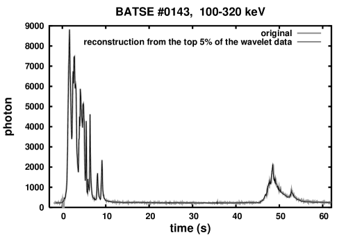
Figure 1: The original and the reconstructed ligthcurve of BATSE trigger 0143 - only 5% of the total wavelet data is used.

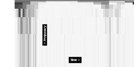
Figure 2: The wavelet phase-space density for BATSE trigger 0143.

3 Wavelet scale analysis

For a frequency-like wavelet scale analysis we would like to create a power-spectrum like distribution along the frequency axis. However, one should be careful. In the classical signal processing one uses the power spectrum from the Fourier-transform, because the signals are electromagnetic-like usually, e.g. the power (or energy) is proportional to the square of the signal. Here the lightcurves measure photon counts — so the signal’s energy is simply the sum of the counts. For this reason we approximate the signal’s strength as a sum the magnitude of the coefficients along the given frequency rows.

Figure 3: The wavelet signal’s frequency distribution for BATSE triggers 0143 and 7343 respectively.

This signal’s strength indicate on Fig 3. (BATSE trigger 0143) the maximum power to be around $f\approx 500\mbox{Hz}$. In each energy channel the signals are similar (observe the logarithmic scale), because the signal is strong even at high energies (channel 4). For BATSE trigger 7343 (with optical redshift $z=1.6006$) one can observe a strong high frequency cutoff: some of the signal’s high frequency part is missing. However all the 4 channels are visible, while the maximum power is around $f\approx 62.5\mbox{Hz}$. It is interesting to remark that the signal’s shape is quite similar to trigger 0143 if that is scaled down by a factor of $\approx 2.4-2.8$ in frequency.

4 Wavelet filtering and similarity

The FRED wavelet transform measures the similarity between the different wavelet kernel functions (here all are FRED-based) and the actual signal. To quantify the similarity we define a magnitude cutoff in the wavelet space so, that the reconstructed $T_{50}$ value from the filtered data should be similar to the original values. The $T_{50}$ value and its $\sigma_{P}$ error from the photon count statistics could be easily determined from the original ligthcurve. To keep only the important features we define the $T_{50\mbox{break}}$ breakpoint where

$$\mid T_{50\mbox{break}}-T_{50}\mid=10.0\sigma_{P}$$

Using a cut-off point it is possible to define a Compressed Size (CS) for a burst: it is the number of bins (in the wavelet space) needed to restore the curve at the break.

The CS value is a robust measure quantifying the similarity between the FRED kernel and the different channels’ lightcurves. Our analysis suggest that all the low energy channels #1, #2 and #3 behaves similarly, while the high energy ($>320$ keV) channel is different (which is not very surprising, e.g. Bagoly et al. (1998)). Fig. 4. shows the ratio of the CS’s against the total count lightcurves’ CS for channels 2 and 4. This distributions indicate that the pulse-shapes in the long bursts’ high energy channel are more FRED-like than the lower ones - and this is independent from the actual FRED time-scale!

Figure 4: The relative value of the CS’s against the total lightcurves’ CS for channels 2 and 4.

References

- Bagoly et al. (1998) Bagoly, Z., Mészáros, A., Horváth, I., Balázs, L. G., & Mészáros, P. 1998, ApJ, 498, 342.
- Kouveliotou et al. (1993) Kouveliotou, C., Meegan, C.A. & Fishman, G.J. 1993, ApJ, 413, L101
- Kouveliotou et al. (1992) Kouveliotou, C., Paciesas, W. S., Fishman, G. J., Meegan, C. A., & Wilson, R. B. 1992, The Compton Observatory Science Workshop, 61
- Meegan et al. (2000) Meegan, C., Malozzi, R.S., Six, F. & Connaughton, V. 2001, Current BATSE Gamma-Ray Burst Catalog, http://gammaray.msfc.nasa.gov/batse/grb/catalog
- Norris et al. (1994) Norris, J. P., Nemiroff, R. J., Bonnell, J. T., Paciesas, W. S., Kouveliotou, C., Fishman, G. J., & Meegan, C. A. 1994, American Astronomical Society Meeting, 26, 1333
- Norris, Scargle, Bonnell, & Nemiroff (1998) Norris, J. P., Scargle, J. D., Bonnell, J. T., & Nemiroff, R. J. 1998, Gamma-Ray Bursts, 4th Hunstville Symposium, 171
- Press et al. (1992) Press W.H., Teukolsky S.A., Vetterling W.T., Flannery B.P. 1992, Numerical Recipes in Fortran, Second Edition, Cambridge University Press, Cambridge
- Quilligan et al. (2002) Quilligan, F., McBreen, B., Hanlon, L., McBreen, S., Hurley, K. J. & Watson, D., 2002, A&A, 385, 377