A Possible Origin of Magnetic Fields in Galaxies and Clusters: Strong Magnetic fields at $z\sim 10$?

Abstract

We propose that strong magnetic fields should be generated at shock waves associated with formation of galaxies or clusters of galaxies by the Weibel instability, an instability in collisionless plasmas. The strength of the magnetic fields generated through this mechanism is close to the order of those observed in galaxies or clusters of galaxies at present. If the generated fields do not decay rapidly, this indicates that strong amplification of magnetic fields after formation of galaxies or clusters of galaxies is not required. This mechanism could have worked even at a redshift of $\sim 10$, and therefore the generated magnetic fields may have affected the formation of stars in protogalaxies. This model will partially be confirmed by future observations of nearby clusters of galaxies. Mechanisms that preserve the magnetic fields for a long time without considerable decay are discussed.

1 Introduction

The question of the origin of galactic magnetic fields is one of the most challenging problems in modern astrophysics. It is generally assumed that magnetic fields in spiral galaxies are amplified and maintained by a dynamo through rotation of the galaxies (Widrow, 2002). The dynamo requires seed fields to be amplified. However, observations of microgauss fields in galaxies at moderate redshifts strongly constrain the lower boundary of the seed fields (Athreya et al., 1998). Moreover, magnetic fields are also observed in elliptical galaxies and galaxy clusters, in which rotation cannot play a central role as the dynamo mechanism (Clarke, Kronberg, & Böhringer, 2001; Widrow, 2002; Vallée, 2004).

The Weibel instability is another mechanism to generate strong magnetic fields (Weibel, 1959; Fried, 1959). This instability is driven in a collisionless plasma, or a tenuous ionised gas, by the anisotropy of the particle velocity distribution function (PDF) of the plasma. When the PDF is anisotropic, currents and then magnetic fields are generated in the plasma so that the plasma particles are deflected and the PDF becomes isotropic (Medvedev & Loeb, 1999). Through the instability, the free energy attributed to the PDF anisotropy is transferred to magnetic field energy. This instability does not need seed magnetic fields. It can be saturated only by nonlinear effects, and thus the magnetic fields can be amplified to very high values. This instability has been observed directly in recent laser experiments (Wei et al., 2002). In astrophysical plasmas, the instability is expected to develop at shocks or at steep temperature gradients, where the PDF is anisotropic. Examples of the sites are pulsar winds, shocks produced by gamma-ray bursts, jets from active galactic nuclei (AGNs), cosmological shocks, and cold fronts (contact discontinuities between cold and hot gas) in clusters of galaxies (Medvedev & Loeb, 1999; Kazimura et al., 1998; Nishikawa et al., 2003; Schlickeiser & Shukla, 2003; Okabe & Hattori, 2003). Although the instability was found in 1959, its nonlinear nature had prevented us from understanding its long-term evolution. Recently, however, as computer power increases, detailed particle simulations of plasmas have been initiated and they have revealed the evolution of magnetic fields even after saturation of the instability (Silva et al., 2003; Medvedev et al., 2005). Based on these results, we consider the generation of magnetic fields at galaxy and cluster-scale shocks through the Weibel instability at the formation of galaxies (both ellipticals and spirals) and clusters. We use the cosmological parameters of $\Omega_{0}=0.3$, $\lambda=0.7$, the Hubble constant of $H_{0}=70\rm\>km\>s^{-1}\>Mpc^{-1}$, and $\sigma_{8}=0.9$.

2 Models

2.1 Generation of Magnetic Fields at Shocks

At the vicinity of the shock front of a collisionless shock, particles from the upstream are mixed up with those in the downstream, and an anisotropy of PDF will be generated in the plasma. As discussed by Schlickeiser & Shukla (2003), the particles from the upstream region firstly will be affected by the Langmuir instability. Since the Langmuir instability is a longitudinal electrostatic mode, the velocity component parallel to the shock normal will be thermalized, while the other components will remain unaffected. Therefore, it is natural to assume that the thermal velocity parallel to the shock normal is on the order of the relative velocity between the upstream and the downstream or on the order of the shock velocity $V_{\mathrm{sh}}$, and those perpendicular to the shock normal are on the order of the thermal velocity of the upstream plasma. This velocity or temperature anisotropy should develop the Weibel instability.

For shocks in electron-proton plasmas, Schlickeiser & Shukla (2003) indicated that the temperature anisotropy for electrons is too small to drive the Weibel instability if $\mathcal{M}\la(m_{\mathrm{p}}/m_{\mathrm{e}})^{1/2}=43$, where $\mathcal{M}=V_{\mathrm{sh}}/v_{\mathrm{th,p}}$ is the shock Mach number, $v_{\mathrm{th,p}}$ is the proton thermal velocity in the upstream, and $m_{\mathrm{p}}$ and $m_{\mathrm{e}}$ are the mass of a proton and that of an electron, respectively. However, if $\mathcal{M}\ga 2$ (note that $\mathcal{M}$ provides a measure of the anisotropy in protons), the temperature anisotropy for the protons is large enough to drive the Weibel instability; this is the case, even if the PDF of the electrons is completely isotropic (see Appendix A).

The magnetic field strength reaches its maximum when the Weibel instability saturates, and the saturation level would be given as follows. As the Weibel instability develops, magnetic fields are generated around numerous current filaments (Medvedev et al., 2005; Kato, 2005). The instability saturates when the generated magnetic fields eventually interrupt the current in each filament, or in other words when the particle’s gyroradii in the excited magnetic fields are comparable to the characteristic wavelength of the excited field (Medvedev & Loeb, 1999). For electron-positron plasmas, Kato (2005) showed that the typical current at and after the saturation is given by the Alfvén current (Alfvén, 1939). In terms of the Alfvén current, the saturated magnetic field strength is given by

$$B_{\mathrm{sat}}\sim\sqrt{2}I_{A}/(\tilde{R}c),$$ (1)

where $\tilde{R}$ is the typical radius of a current filament at the saturation and $I_{A}\equiv\langle v_{\parallel,\rm e}/c\rangle m_{\mathrm{e}}c^{3}/e$ is the Alfvén current (for nonrelativistic cases). Here, $v_{\parallel,\rm e}$ is the electron thermal velocity in the direction of the higher temperature. For strongly anisotropic cases (i.e., the particle limit cases discussed by Kato, 2005), the radius at the saturation is given by $\tilde{R}\sim 2c/\omega_{\rm pe}$, where $\omega_{\rm pe}\equiv(4\pi n_{\mathrm{e}}e^{2}/m_{\mathrm{e}})^{1/2}$ is the electron plasma frequency, and the saturated magnetic field strength is given by

$$B_{\mathrm{sat}}\sim 0.5\ v_{\parallel,\rm e}\ (4\pi n_{\mathrm{e}}m_{\mathrm{e}})^{1/2},$$ (2)

where $n_{\mathrm{e}}$ is the electron number density.

For electron-proton plasmas we consider below, currents carried by heavier protons will generate stronger magnetic fields at the saturation. It is natural to assume that the saturation for the proton currents is determined by the Alfvén current defined for protons, $I^{\prime}_{A}\equiv\langle v_{\parallel,\rm p}/c\rangle m_{\mathrm{p}}c^{3}/e$, where $v_{\parallel,\rm p}$ is the proton thermal velocity in the direction of the higher temperature. In a shock wave, this leads to

$$B_{\mathrm{sat}}\sim 0.5\ V_{\mathrm{sh}}\ (2\pi n_{\mathrm{p}}m_{\mathrm{p}})^{1/2}\>,$$ (3)

where $n_{\mathrm{p}}$ is the proton number density and we used the assumption of $v_{\parallel,\rm p}\sim V_{\mathrm{sh}}$. This expression is valid when the PDF of the protons has a strong anisotropy or $\mathcal{M}\ga 2$ (Kato, 2005). Note that the energy density of the saturated magnetic fields attains to a sub-equipartition level with the particle kinetic energy. The numbers in the parentheses in equations (2) and (3) are different by a factor of two, because in electron-positron plasmas, both electron and positron compose currents at the same time, while in electron-proton plasmas, only protons contribute to currents when the proton Weibel instability develops. In electron-proton plasmas, if electron anisotropy is sufficiently large, electrons first generate magnetic fields, which saturate at the early stage of the instability, and then protons generate magnetic fields, which leads to the second saturation. Such an evolution was also observed in numerical simulations (Frederiksen et al., 2004).

The magnetic fields generated at the shock front will be convected downstream at the fluid velocity (in the shock rest frame). At least for a short period after the saturation, the magnetic field strength decreases as the current filaments merge together, because the current in each filament is limited to the proton Alfvén current while the size of the current filaments increases (Kato, 2005). However, the long-term evolution is still an open question. Medvedev et al. (2005) indicated that the field should reach an asymptotic value beyond which it will not decay, although their model can be applied only when currents are not dissipated. Recent particle simulations have also shown that the final magnetic field strength is given by $B_{f}=\eta_{\rm mer}^{1/2}B_{\mathrm{sat}}$, where $\eta_{\rm mer}\sim 0.01$ (Silva et al., 2003; Medvedev et al., 2005). In the following, we assume that the magnetic fields of $B_{f}$ are preserved. The very long-term evolution of the magnetic fields, for which the results of Medvedev et al. (2005) and Silva et al. (2003) cannot be directly applied, will be discussed in Section 4.

We note that unfortunately, at present, most simulations treat electron-positron shocks and there are virtually no simulations that reveal the evolution of collisionless electron-proton shocks satisfactorily (in terms of box sizes, duration times, and so on), because of the lack of computational power. Therefore, the model stated above and used in this paper should be confirmed by direct numerical simulations in the future.

2.2 Shock Formation

According to the standard hierarchical clustering scenario of the universe, an initial density fluctuation of dark matter in the universe gravitationally grows and collapses; its evolution can be approximated by that of a spherical uniform over-dense region (Gunn & Gott, 1972; Peebles, 1980). The collapsed objects are called ‘dark halos’ and the gas in these objects later forms galaxies or clusters of galaxies. At the collapse, the gas is heated by the ‘virial shocks’ to the virial temperature of the dark halo, $T_{\rm vir}=GM/(2r_{\rm vir})$, where $G$ is the gravitational constant, and $M$ and $r_{\rm vir}$ are the mass and the virial radius of the dark halo, respectively. The relation between the virial radius and the virial mass of an object is given by

$$r_{\rm vir}=\left[\frac{3\>M}{4\pi\Delta_{c}(z)\rho_{\rm crit}(z)}\right]^{1/3}\>,$$ (4)

where $\rho_{\rm crit}(z)$ is the critical density of the universe, and $\Delta_{c}(z)$ is the ratio of the average density of the object to the critical density at redshift $z$. The critical density depends on redshift because the Hubble constant depends on that, and it is given by

$$\rho_{\rm crit}(z)=\frac{\rho_{\rm crit,0}\Omega_{0}(1+z)^{3}}{\Omega(z)}\>,$$ (5)

where $\rho_{\rm crit,0}$ is the critical density at $z=0$, and $\Omega(z)$ is the cosmological density parameter given by

$$\Omega(z)=\frac{\Omega_{0}(1+z)^{3}}{\Omega_{0}(1+z)^{3}+\lambda}$$ (6)

for the flat universe with non-zero cosmological constant. The ratio $\Delta_{c}(z)$ is given by

$$\Delta_{c}(z)=18\>\pi^{2}+82x-39x^{2}\>,$$ (7)

for the flat universe (Bryan & Norman, 1998), where the parameter $x$ is given by $x=\Omega(z)-1$. The virial shocks form at $r\approx r_{\rm vir}$ and the velocity is $v_{\rm vir}\approx\sqrt{GM/r_{\rm vir}}$.

In addition, recent cosmological numerical simulations have shown that ‘large-scale structure (LSS) shocks’ form even before the collapse (Cen & Ostriker, 1999; Miniati et al., 2000; Davé et al., 2001; Ryu et al., 2003). They form at the turnaround radius ($r_{\rm ta}\sim 2r_{\rm vir}$), the point at which the density fluctuation breaks off from the cosmological expansion. For simplicity, we assume that $r_{\rm ta}=2r_{\rm vir}$, which is close to the self-similar infall solution for a particular mass shell in the Einstein-de Sitter Universe ($r_{\rm ta}=1/0.56\>r_{\rm vir}$; Bertschinger, 1985). The gas that later forms a galaxy or a cluster passes two types of shocks; first, the gas passes the outer LSS shock, and then, the inner virial shock. The typical velocity of the LSS shocks is $V_{\mathrm{sh}}\approx H(z)r_{p}$ (Furlanetto & Loeb, 2004), where $H(z)$ is the Hubble constant at redshift $z$, and $r_{p}$ is the physical radius that the region would have had if it had expanded uniformly with the cosmological expansion. The temperature of the postshock gas is $T_{s}\approx 3/16\>(\mu m_{\mathrm{p}}/k_{\mathrm{B}})V_{\mathrm{sh}}^{2}$, where $\mu m_{\mathrm{p}}$ is the mean particle mass, and $k_{\mathrm{B}}$ is the Boltzmann constant. Note that although the model of Furlanetto & Loeb (2004) has been compared with numerical simulations at $z\sim 0$, it has not been at high-redshifts; it might have some ambiguity there. We do not consider mergers of objects that have already collapsed as the sites of magnetic field generation because the Weibel instability applies only to initially unmagnetised or weakly magnetised plasmas; at the merger, collapsed objects just bring their magnetic fields to the newly born merged object.

Since the Weibel instability develops in ionised gas (plasma), we need to consider the ionisation history of the universe. After the entire universe is ionised by stars and/or AGNs ($z\la 8$), magnetic fields are first generated at the LSS shocks. In this case, we do not consider the subsequent generation of magnetic fields at the inner virial shocks, because the strength is at most comparable to that of the magnetic fields generated at the LSS shocks. On the other hand, when the universe is not ionised ($z\ga 8$), the Weibel instability cannot develop at the outer LSS shocks. However, if the LSS shocks heat the gas (mostly hydrogen) to $T_{s}>10^{4}{\rm\>K}$ and ionise it, the instability can develop at the inner virial shocks.

In this case, the gas ionised at the LSS shock may recombines before it reaches the virial shock. The recombination time-scale is given by

$$\tau_{\rm rec}=\frac{1}{\alpha n_{\mathrm{e}}}\approx 1.22\times 10^{5}\;{\rm yr}\>\frac{1}{y}\left(\frac{T}{\rm 10^{4}K}\right)^{0.7}\left(\frac{n_{\mathrm{H}}}{\rm cm^{-3}}\right)^{-1}\>,$$ (8)

where $\alpha$ is the recombination coefficient, $T$ is the gas temperature, $y$ is the ionisation fraction, and $n_{\mathrm{H}}$ is the hydrogen density (Shapiro & Kang, 1987). If we assume that $\tau_{\rm rec}=\tau_{\rm dyn}$, where $\tau_{\rm dyn}\approx(1/2)r_{\rm ta}/V_{\mathrm{sh}}$ is the time-scale that the gas moves from the LSS shock to the virial shock, the ionisation rate when the gas reaches the virial shock is

$$y\approx\left(\frac{\tau_{\rm dyn}}{1.22\times 10^{5}\;{\rm yr}}\right)^{-1}\left(\frac{T}{\rm 10^{4}K}\right)^{0.7}\left(\frac{n_{\mathrm{H}}}{\rm cm^{-3}}\right)^{-1}\;$$ (9)

for $y<1$. We found that $y<1$ for $z\ga 9$, and the minimum value when the generation of magnetic fields is effective ($z\la 12$, see §3) is $y\sim 0.3$. When $y<1$, we simply replace $n_{\mathrm{p}}$ in equation (3) with $yn_{\mathrm{H}}$. For temperature, we assumed that $T=T_{s}$ in equation (9). Since the magnetic fields do not much depend on the temperature ($B_{\mathrm{sat}}\propto y^{0.5}\propto T^{0.35}$), they do not much change even when radiative cooling reduces the temperature; at least $B_{\mathrm{sat}}$ does not change by many orders of magnitude. It was shown that the ionisation rate just behind a shock is $y\sim 0.1$, if the shock velocity is relatively small ($V_{\mathrm{sh}}\sim 40\rm\;km\;s^{-1}$; Shapiro & Kang, 1987; Susa et al., 1998). If the shock velocity is larger, $y\sim 1$. In our calculations, the velocity of the LSS shocks is $V_{\mathrm{sh}}\ga 40\rm\;km\;s^{-1}$, when the generation of magnetic fields is effective. Thus, $y$ just behind the shocks is at least comparable to that obtained through the condition of $\tau_{\rm rec}\sim\tau_{\rm dyn}$, and the incomplete ionisation does not much affect the results shown in the next section (see also Section 4).

3 Results and Discussion

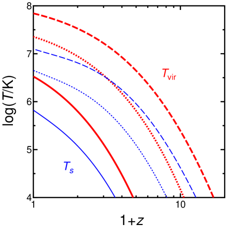
Fig.1 shows the typical mass of objects, $M$, as a function of redshift $z$; the labels $1\sigma$, $2\sigma$, and $3\sigma$ indicate the amplitudes of initial density fluctuations in the universe from which the objects form, on the assumption of the CDM fluctuations spectrum (Barkana & Loeb, 2001). Fig.2 shows the downstream temperature at the virial shock ($T_{\rm vir}$) and that at the LSS shock ($T_{s}$) for the objects; $T_{\rm vir}$ is always larger than $T_{s}$. The ratio $T_{\rm vir}/T_{s}$ indicates that ${\cal M}\ga 4$ for the virial shock. For the LSS shock, ${\cal M}\gg 1$, because the gas outside the shock is cold. Thus, equation (3) can be applied to both shocks. In Fig.3, we present the strength of magnetic fields ($B_{c}$) at a scale of $r_{\rm vir}$ for the collapsed objects. We assume that the entire universe is reionised at $z=8$. Thus, for $z>8$, magnetic fields are generated only at the virial shocks if $T_{s}>10^{4}\rm\>K$. We assume that $B_{c}=B_{f}$ and plot the lines only when $T_{s}>10^{4}\rm\>K$. The recombination is effective at $z>10$ for the $3\sigma$ model. On the other hand, for $z<8$, the magnetic fields are generated at the LSS shocks. We consider the compression of the fields while the size of the gas sphere decreases from $r=r_{\rm ta}$ to $r=r_{\rm vir}$, and thus we assume that $B_{c}=8^{2/3}\>B_{f}$. Moreover, we plot the lines only for $T_{\rm vir}>2\times 10^{5}$ K, because below this temperature, gas infall is suppressed by photoionisation heating (Efstathiou, 1992; Furlanetto & Loeb, 2004).

Figure 1: Typical masses of objects forming at redshift $z$. The labels, $1\sigma$, $2\sigma$, and $3\sigma$ (solid, dotted, and dashed lines, respectively) indicate the amplitudes of initial density fluctuations from which the objects formed; $\sim 1$–$3\sigma$ is the typical value (Barkana & Loeb, 2001). Objects with masses of $M\la 10^{12}\>M_{\odot}$ and $M\ga 10^{13}\>M_{\odot}$ correspond to galaxies (ellipticals and spirals) and clusters of galaxies, respectively.

Figure 2: Temperatures behind the virial shocks ($T_{\rm vir}$; thick lines) and those behind the LSS shocks ($T_{s}$; thin lines) for objects forming at redshift $z$. Solid, dotted, and dashed lines correspond to $1\sigma$, $2\sigma$, and $3\sigma$ fluctuations, respectively (see Fig.1)

Figure 3: Typical magnetic field strengths of objects forming at redshift $z$. Solid, dotted, and dashed lines correspond to $1\sigma$, $2\sigma$, and $3\sigma$ fluctuations, respectively (see Fig.1).

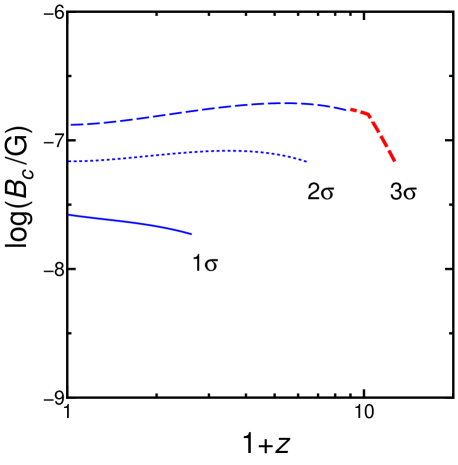
In Fig.3, the strength of magnetic fields generated by protons reaches $\sim 10^{-8}$–$10^{-7}$ G and is very close to the values observed in nearby galaxies and clusters of galaxies ($\sim 10^{-6}$ G; Clarke et al., 2001; Widrow, 2002; Vallée, 2004). On a galactic scale, the gas sphere may further contract to $r\ll r_{\rm vir}$ because of radiative cooling. If magnetic fields are frozen in the gas, the strength exceeds $\sim 10^{-6}$ G. However, if this happens, the magnetic energy exceeds the thermal or kinetic energy of the gas. As a result, magnetic reconnection may reduce the strength. In fact, the equipartition between the magnetic energy density and the thermal or kinetic energy density appears to be held in the Galaxy (Beck et al., 1996).

The strong magnetic fields shown in Fig. 3 indicate that strong amplification of magnetic fields, such as dynamo amplification, is not required after formation of the galaxies and clusters. This is consistent with the observations of galactic magnetic fields at $z\ga 2$ (Athreya et al., 1998). Future observations of higher-redshift galaxies would discriminate between our model and strong dynamo amplification models; the latter predict much weaker magnetic fields at higher redshifts. Moreover, since the predicted galactic magnetic fields are comparable to those at present, they might have affected the formation of stars in protogalaxies. Fig.3 also shows that our model naturally explains the observational fact that the magnetic field strengths of galaxies and galaxy clusters fall in a small range (a factor of 10). Since our model predicts that magnetic fields are generated around objects, magnetic fields in intergalactic space are not required as the seed or origin of galactic magnetic fields.

Some recent numerical simulations indicated that gas is never heated to $\sim T_{\rm vir}$ for less massive objects because radiative cooling is efficient and the shocks forming at $\ga r_{\rm vir}$ are unstable (Birnboim & Dekel, 2003; Kereš et al., 2005). This effect may be important for $M\la 10^{12}\>M_{\odot}$. If it is correct, the generation of magnetic fields is only effective for $z\la 5$ (the $3\sigma$ curve in Fig. 1). However, even for $M\la 10^{12}\>M_{\odot}$, multiple shocks may form at the inner halo when the cold gas reaches there and collides each other (Kereš et al., 2005). Therefore, magnetic fields may be created there. The details of these shocks could be studied by high-resolution numerical simulations.

Although it would be difficult to directly observe the generation of magnetic fields through the Weibel instability for distant high-redshift galaxies, it would be easier for nearby clusters of galaxies. Since clusters are now growing, LSS shocks should be developing outside of the virial radii of the clusters (Miniati et al., 2000; Ryu et al., 2003). Since particles are often accelerated at shocks, the synchrotron emission from the accelerated particles could be observed with radio telescopes with high sensitivity at low frequencies (Keshet, Waxman, & Loeb, 2004). The total non-thermal luminosity (synchrotron luminosity plus inverse Compton scattering with cosmic microwave background [CMB] photons) is estimated as

$$L_{\rm nt}\approx\frac{\epsilon}{r_{\rm ta}/u}\frac{fM}{m_{\mathrm{p}}}\frac{1}{2}V_{\mathrm{sh}}^{2}\>,$$ (10)

where $\epsilon$ is the acceleration efficiency and $f$ is the gas fraction of a cluster. If we assume $\epsilon=0.03$ (Tanimori et al., 1998; Muraishi et al., 2000) and $f=0.15$ (Mohr, Mathiesen, & Evrard, 1999), the maximum value of $L_{\rm nt}$ is $\sim 10^{43}\rm\>erg\>s^{-1}$. Since the energy density of magnetic fields ($u_{\rm B}$) is smaller than that of the CMB ($u_{\mathrm{CMB}}$), most of the non-thermal luminosity ($L_{\rm nt}$) is attributed to the inverse Compton scattering such as $u_{\mathrm{CMB}}L_{\rm nt}/(u_{\rm B}+u_{\mathrm{CMB}})$, which may have been detected in the hard X-ray band ($\ga 20$ keV; Fusco-Femiano et al., 2004). Thus, the synchrotron radio luminosity is $u_{\rm B}L_{\rm nt}/(u_{\rm B}+u_{\mathrm{CMB}})\la 10^{39}\rm\>erg\>s^{-1}$. Some of the diffuse radio sources observed in the peripheral cluster regions (‘radio relics’) may be this emission (Govoni & Feretti, 2004). Since the Weibel instability generates magnetic fields on the plane of the shock front, the synchrotron emission should be polarised perpendicular to the shock front (Medvedev & Loeb, 1999), which is actually observed for some radio relics (Govoni & Feretti, 2004). The synchrotron emission will tell us the positions of the LSS shocks, if they exist. If magnetic fields are generated there, they should be observed only downstream of the shock. This may be confirmed through Faraday rotation measurements of radio sources behind the cluster for both sides of the shock, if the coherent length of the fields sufficiently increases (see Section 4).

4 On the long-term evolution of magnetic fields

The model proposed here has large uncertainties, especially on the very long-term (say Gyr) evolution of magnetic fields. The typical time-scale of the Weibel instability until the saturation is given by the inverse of the proton plasma frequency, $\omega_{\rm pp}\equiv(4\pi n_{\mathrm{p}}e^{2}/m_{\mathrm{p}})^{1/2}$. However, it is evident that this time-scale is much smaller than the cosmological time-scale we have considered in this paper. The typical scale-length of the saturated fields is given by the proton inertial length $c/\omega_{\rm pp}$, and it is also much smaller than a kpc scale. Thus, there is a ‘missing link’ between the generated fields and those observed in galaxies and clusters at present.

If the observed magnetic fields have their origin in the Weibel instability, there should be another mechanism that takes over the instability. If the saturation and current evolution model of Kato (2005) is applied to proton currents, the magnetic field strength should decrease after the saturation as

$$B=B_{\mathrm{sat}}\ (R/\tilde{R})^{-1},$$ (11)

where $R$ is the radius of a filament, and the filament radius at saturation, $\tilde{R}$, is defined for protons ($\tilde{R}\sim 2c/\omega_{\rm pp}$). This is because the current strength is limited to the proton Alfvén current $I^{\prime}_{A}$ while the radius of current filaments increases through mergers of the filaments. Since $\tilde{R}\sim 10^{10}\mathrm{cm}$ for $n_{\mathrm{p}}\sim 10^{-5}\mathrm{cm}^{-3}$ (at $r\sim r_{\rm vir}$ for a cluster at $z\sim 0$), the magnetic field strength should be reduced by a factor of $\sim 10^{11}$, if relation (11) holds even for an long-term evolution to a kpc ($\sim 10^{21}$ cm) scale field.

One possibility to overcome this difficulty is that the currents are carried in another form at later times. At early times of the evolution, the state of the plasma is in a kinetic regime in which the characteristic scale of magnetic fields is comparable to or smaller than the Larmor radius of particles. Probably, at later times, the former would increase via current mergers, and would become larger than the latter. After this situation is realised, the straight currents generated by the Weibel instability, which are limited to the Alfvén current, might be superseded by a kind of drift currents, and the plasma might behave as a MHD fluid. In this case, mergers of the cylindrical structures, which were originally the current filaments, would occur through the reconnection process as usually considered for MHD fluids, and therefore the magnetic field strength would not decrease considerably unless the diffusion of magnetic fields owing to collisions between charged particles or collisions with neutrals becomes effective. This would allow the magnetic fields to survive for a long time. For example, in a MHD fluid, for the scale of $L\sim 10^{10}\rm\>cm$ and the temperature of a few keV, the dissipation time-scale of magnetic fields through the collisions between charged particles is $t_{\rm diss}\sim 10^{9}$ yr (Spitzer, 1962), which is the dynamical time-scale of a cluster. If current mergers make $L$ larger, $t_{\rm diss}$ also becomes larger. The numerical simulations performed by Silva et al. (2003) showed that magnetic fields do not much decay after the saturation. This might reflect the transition to a MHD fluid. Moreover, a MHD inverse cascade mechanism (e.g. Vishniac & Cho, 2001) could provide another process to make larger-scale magnetic fields observed in galaxies and clusters ($\ga$ kpc). Since the ionisation rate, $y$, is fairly large (Section 2.2), the ambipolar diffusion of magnetic fields (the collisions with neutrals) can be ignored (e.g. eq. 13–57 in Spitzer, 1978). At any rate, studies about the long-term evolution of magnetic fields are strongly encouraged.

5 Conclusions

In this paper, we showed that the Weibel instability can generate strong magnetic fields in shocks around galaxies and clusters. The strength is comparable to those observed in galaxies and clusters at present. The mechanism could have worked even at $z\sim 10$. The results are based on the assumption that the magnetic fields generated by the Weibel instability are conserved for a long time. The validity of this assumption must be confirmed in future studies.

Appendix A Dispersion relation of the Weibel instability

Here, we derive the dispersion relation of the Weibel instability in a plasma which consists of some species (or populations) of charged particles. In the following, each species is denoted by a label ‘s’ (s = e for electron, p for proton, and so on), and the mass, charge, and number density of the species are denoted by $m_{\mathrm{s}}$, $q_{\mathrm{s}}$ and $n_{\mathrm{s}}$, respectively. We assume here that each species has a bi-Maxwellian distribution

$$f_{0}^{(\mathrm{s})}(\mathbf{v})=\frac{n_{\mathrm{s}}}{(2\pi)^{3/2}\alpha_{\mathrm{s}}\sigma_{\mathrm{s}}^{3}}\exp\left[-\frac{v_{x}^{2}+v_{y}^{2}}{2\sigma_{\mathrm{s}}^{2}}-\frac{v_{z}^{2}}{2\alpha_{\mathrm{s}}^{2}\sigma_{\mathrm{s}}^{2}}\right],$$ (12)

where the thermal velocity is given by $\sigma_{\mathrm{s}}$ for $x$ or $y$ directions, and it is given by $\alpha_{\mathrm{s}}\sigma_{\mathrm{s}}$ for $z$ direction.

If the thermal velocity in $z$ direction is larger than the other directions , that is, $\alpha_{\mathrm{s}}\geq 1$, the linear dispersion relation of the Weibel mode, which is relevant to the $z$ component of the current density, is given as

$$\omega^{2}-(ck)^{2}+\sum_{\mathrm{s}}\omega_{\mathrm{ps}}^{2}\left[\alpha_{\mathrm{s}}^{2}\zeta_{\mathrm{s}}Z(\zeta_{\mathrm{s}})+\alpha_{\mathrm{s}}^{2}-1\right]=0,$$ (13)

where

$$\omega_{\mathrm{ps}}\equiv\sqrt{\frac{4\pi n_{\mathrm{s}}q_{\mathrm{s}}^{2}}{m_{\mathrm{s}}}},\qquad\zeta_{\mathrm{s}}\equiv\frac{\omega}{k\sqrt{2}\sigma_{\mathrm{s}}},$$ (14)

and $Z(\zeta)$ is the plasma dispersion function defined as

$$Z(\zeta)\equiv\frac{1}{\sqrt{\pi}}\int_{-\infty}^{\infty}\frac{1}{z-\zeta}e^{-z^{2}}dz.$$ (15)

It is shown that the dispersion relation (13) can have purely positive-imaginary solution of $\omega$, i.e., purely growing mode. Since the growth rate becomes zero at the maximum wave number of the unstable mode, $k_{\mathrm{max}}$, we can set $\omega=0$ and $\zeta_{\mathrm{s}}Z(\zeta_{\mathrm{s}})=0$ at $k=k_{\mathrm{max}}$ in Eq.(13) to obtain

$$k_{\mathrm{max}}^{2}=\frac{1}{c^{2}}\sum_{\mathrm{s}}\omega_{\mathrm{ps}}^{2}(\alpha_{\mathrm{s}}^{2}-1).$$ (16)

It is evident that there is no unstable mode if $k_{\mathrm{max}}^{2}\leq 0$, while unstable modes exist if $k_{\mathrm{max}}^{2}>0$. Explicitly, the condition for instability is given by

$$\sum_{\mathrm{s}}\omega_{\mathrm{ps}}^{2}(\alpha_{\mathrm{s}}^{2}-1)>0.$$ (17)

It should be noted that, in an electron-proton plasma for example, even when the electron distribution is completely isotropic ($\alpha_{\mathrm{e}}=1$) at the initial time, unstable modes exist if the proton distribution is anisotropic ($\alpha_{\mathrm{p}}>1$).

The above results show that even if the Mach number of a shock is relatively small ($\alpha_{\mathrm{e}}\approx 1$), the magnetic fields generated by the anisotropy of proton distribution slowly grow and reach the saturation value given by equation (3) (Kato, 2005).

References

- Alfvén (1939) Alfvén H., 1939, Phys. Rev., 55, 425
- Athreya et al. (1998) Athreya R. M., Kapahi V. K., McCarthy P. J., van Breugel W., 1998, A&A, 329, 809
- Barkana & Loeb (2001) Barkana R., Loeb A., 2001, Physics Reports, 349, 125
- Beck et al. (1996) Beck R., Brandenburg A., Moss D., Shukurov A., Sokoloff D., 1996, ARA&A, 34, 155
- Bertschinger (1985) Bertschinger E., 1985, ApJS, 58, 39
- Birnboim & Dekel (2003) Birnboim Y., Dekel A., 2003, MNRAS, 345, 349
- Bryan & Norman (1998) Bryan G. L., Norman M. L., 1998, ApJ, 495, 80
- Cen & Ostriker (1999) Cen R., Ostriker J. P., 1999, ApJ, 519, L109
- Clarke et al. (2001) Clarke, T. E., Kronberg, P. P., & Böhringer, H. 2001, ApJ, 547, L111
- Davé et al. (2001) Davé R., et al., 2001, ApJ, 552, 473
- Davidson et al. (1972) Davidson, R. C., Hammer, D. A., Haber, I., Wagner, C. E. 1972, Phys. Fluids, 317, 333
- Efstathiou (1992) Efstathiou, G. 1992, MNRAS, 256, 43P
- Frederiksen et al. (2004) Frederiksen, J. T., Hededal, C. B., Haugbølle, T., Nordlund, Å. 2004, ApJ, 608, L13
- Fried (1959) Fried, B. D. 1959, Phys. Fluids, 2, 83
- Furlanetto & Loeb (2004) Furlanetto, S. R., Loeb, A. 2004, ApJ, 611, 642
- Fusco-Femiano et al. (2004) Fusco-Femiano, R., Orlandini, M., Brunetti, G., Feretti, L., Giovannini, G., Grandi, P., Setti, G. 2004, ApJ, 602, L73
- Govoni & Feretti (2004) Govoni, F., Feretti, L. 2004, Int. J. Mod. Phys. D13 1549
- Gunn & Gott (1972) Gunn, J. E., Gott, J. R. I. 1972, ApJ, 176, 1
- Kato (2005) Kato, T. N., 2005, Phys. Plasmas, 12, 080705
- Kazimura et al. (1998) Kazimura, Y., Sakai, J. I., Neubert, T., Bulanov, S. V. 1998, ApJ, 498, L183
- Kereš et al. (2005) Kereš, D., Katz, N., Weinberg, D. H., Davé, R. 2005, MNRAS in press (astro-ph/0407095)
- Keshet et al. (2004) Keshet, U., Waxman, E., Loeb, A. 2004, ApJ, 617, 281
- Medvedev et al. (2005) Medvedev, M. V., Fiore, M., Fonseca, R. A., Silva, L. O., Mori, W. B. 2005, ApJ, 618, L75
- Medvedev & Loeb (1999) Medvedev, M. V., Loeb, A. 1999, ApJ, 526, 697
- Miniati et al. (2000) Miniati, F., Ryu, D., Kang, H., Jones, T. W., Cen, R., Ostriker, J. P. 2000, ApJ, 542, 608
- Mohr et al. (1999) Mohr, J. J., Mathiesen, B., Evrard, A. E. 1999, ApJ, 517, 627
- Muraishi et al. (2000) Muraishi, H., et al. 2000, A&A, 354, L57
- Nishikawa et al. (2003) Nishikawa, K.-I., Hardee, P., Richardson, G., Preece, R., Sol, H., Fishman, G. J. 2003, ApJ, 595, 555
- Okabe & Hattori (2003) Okabe, N., & Hattori, M. 2003, ApJ, 599, 964
- Peebles (1980) Peebles, P. J. E. 1980, Large-Scale Structure of the Universe (Princeton Univ. Press; Princeton)
- Petschek (1964) Petschek, H. E. 1964, in The Physics of Solar Flares, ed. W. N. Hess (Washington, DC: NASA), 425
- Ryu et al. (2003) Ryu, D., Kang, H., Hallman, E., Jones, T. W. 2003, ApJ, 593, 599
- Schlickeiser & Shukla (2003) Schlickeiser, R., Shukla, P. K. 2003, ApJ, 599, L57
- Shapiro & Kang (1987) Shapiro, P. R., & Kang, H. 1987, ApJ, 318, 32
- Silva et al. (2003) Silva, L. O., Fonseca, R. A., Tonge, J. W., Dawson, J. M., Mori, W. B., Medvedev, M. V. 2003, ApJ, 596, L121
- Spitzer (1962) Spitzer, Jr. L. 1962, Physics of Fully Ionized Gases (New York: Wiley)
- Spitzer (1978) Spitzer, Jr. L. 1978, Physical Processes in the Interstellar Medium (New York: Wiley)
- Susa et al. (1998) Susa, H., Uehara, H., Nishi, R., Yamada, M. 1998, Progress of Theoretical Physics, 100, 63
- Tanimori et al. (1998) Tanimori, T., et al. 1998, ApJ, 497, L25
- Vallée (2004) Vallée, J. P. 2004, New Astronomy Review, 48, 763
- Vishniac & Cho (2001) Vishniac, E. T., Cho, J. 2001, ApJ, 550, 752
- Wei et al. (2002) Wei, M. S., et al. 2002, Central Laser Facility (UK) Annual Report (http://www.clf.rl.ac.uk/Reports/2001-2002/pdf/10.pdf)
- Weibel (1959) Weibel, E. S. 1959, Phys. Rev. Lett., 2, 83
- Widrow (2002) Widrow, L. M. 2002, Reviews of Modern Physics, 74, 775