Binarity, activity and metallicity among late-type stars

We present the first in a series of papers that attempt to investigate the relation between binarity, magnetic activity, and chemical surface abundances of cool stars. In the current paper, we lay out and test two abundance analysis methods and apply them to two well-known, active, single stars, HD 27536 (G8IV-III) and HD 216803 (K5V), presenting photospheric fundamental parameters and abundances of Li, Al, Ca, Si, Sc, Ti, V, Cr, Fe, Co and Ni. The abundances from the two methods agree within the errors for all elements except calcium in HD 216803, which means that either method yields the same fundamental model parameters and the same abundances. Activity is described by the radiative loss in the Ca ii H&K lines with respect to the bolometric luminosity, through the activity index $R_{\mathrm{HK}}$. Binarity is established by very precise radial velocity (RV) measurements using HARPS spectra. The spectral line bisectors are examined for correlations between RV and bisector shape to distinguish between the effects of stellar activity and unseen companions. We show that HD 27536 exhibit RV variations mimicking the effect of a low-mass ($m\sim 4$ M_J) companion in a relatively close ($a\sim 1$ AU) orbit. The variation is strongly correlated with the activity, and consistent with the known photometric period $P=306.9$ d, demonstrating a remarkable coherence between $R_{\mathrm{HK}}$ and the bisector shape, i.e. between the photosphere and the chromosphere. We discuss the complications involved in distinguishing between companion and activity induced RV variations.

1 Introduction

There is currently still no single theory that adequately describes magnetic activity on cool main-sequence stars with outer convective envelopes. Neither is there a solid description of its impact on stellar evolution. While the current scheme of dynamo models successfully account for the existence of magnetic fields for stars at the age of the Sun, more quantitative explanations are lacking (see Strassmeier 2003, for a recent review).

It has been established empirically (Noyes et al. 1984) that the activity level, and hence the dynamo efficiency, is a monotonic function of the rotation period for stars with periods larger then a few days. It scales approximately with the Rossby number $\mathcal{R}_{0}=P\tau_{c}^{-1}$, where $\tau_{c}$ is the convective turnover time and $P$ the rotational period. Hence, the activity is indirectly a function of the spectral type. However, the boundary layer dynamo model is unable to account for the activity in the overactive M dwarfs, and also the reason for and the exact scaling with $\mathcal{R}_{0}$ is not fully understood (e.g. Schrijver 1996; Schrijver & Zwaan 2000).

Although rotation is thought to be the necessary condition for magnetic activity, it is not clear to what extent binarity influences the generation and morphology of magnetic fields and the corresponding chromospheric and coronal emission (e.g. Bopp & Fekel 1977; Edwards 1983; Shkolnik et al. 2003). The differential gravitational pull from a companion may cause a longitude- and latitude-dependent relationship between rotation rate and activity level, and may also contribute to an inhomogeneous chemical abundance by introducing tidal waves which affect the chemical stratification. No theoretical studies exist in the literature, but if such relationships exist, the models of the evolution of close binaries would then need to be reconsidered.

Another burning question is the link between chemical surface abundances and binarity. The recent observation that (solar-like) stars with planets are on average more metal rich than similar stars without planets (e.g. Santos et al. 2001, 2004, 2005; Fischer et al. 2003) is at least suggestive that this maybe also the case for binaries. Of particular interest is the fact that the Li abundance seem to differ between single stars and stars which host giant planets (Israelian et al. 2004), and even between otherwise identical twin-star binaries (Martín et al. 2002; Dall et al. 2005), possibly related to pre-MS accretion of planetesimals or engulfment of planets.

Furthermore, as instrumentation improves (i.e. HARPS – see Mayor et al. 2003), more and more single stars turn out to have variable radial velocity (RV), due to the presence of low-mass companions, either low-mass stars, brown dwarfs or giant planets. It is thus becoming necessary and indeed possible to deal properly with the effects of binarity, and to attempt to separate the classical dynamo process of internal differential rotation from the external contribution from close companions. In this discussion it is necessary to extend the concept of binarity to include all possible companions, including brown dwarfs and planets.

We are currently conducting a search for true single stars among the known active stars, in order to study the activity-rotation relation in a sample that is not “polluted” by any type of binaries. Furthermore, we may hope to isolate the effects that binarity may have on stellar activity. Our sample consist of about 30 known active G–M stars, with known photometric variations attributed to rotational modulation of star spots, including both binaries and — supposedly — single stars. Most of our sample stars belong to the BY Draconis variables, which are defined from their variability due to changing star spot coverage (Bopp & Fekel 1977). Several aspects need to be investigated to properly analyze the sample, including (1) time-resolved RV monitoring and (2) line bisector analysis, (3) monitoring of activity indexes, (4) determination of fundamental atmospheric parameters, and (5) accurate photospheric abundance analysis. RV variations due to stellar acoustic oscillations, which for our purposes is an additional noise source, are effectively filtered out by the long exposure times typically involved.

In this paper we will investigate various tools available to perform reliable, accurate and fast abundance analysis. Since this will have to be done in detail for all stars in the sample, we are developing ways to perform this task in as automated a way as possible, without employing fully automated procedures yet (e.g. minimum distance methods, see Allende Prieto 2004), although this is eventually the goal. Such automated tools will be of great utility in the future, not least in view of upcoming facilities like STELLA (Strassmeier et al. 2004).

In this paper we present an analysis of the two well-studied active stars HD 27536 and HD 216803, deriving their fundamental atmospheric parameters and their elemental abundances, as well as their activity indexes. So far only very few abundance analyses have been carried out for active stars, mostly due to the complications involved (see e.g. Katz et al. 2003; Morel et al. 2003, for recent applications to RS CVn stars). We furthermore present a preliminary analysis of the time-resolved RV, bisector and activity index data for HD 27536.

A future paper will deal with the full sample of stars addressing the RV, activity, and line bisector variations and the statistical properties of the sample, presenting a discussion of the effects of binarity on the stellar activity.

2 Observations

2.1 The target stars

HD 27536 (EK Eri, HR1362) presents a special case. As shown by Strassmeier et al. (1999) it is a slowly rotating G8 giant with an over-active chromosphere possibly due to a fossil Ap type magnetic field, viewed at an inclination close to 90^∘. The star has a measured rotation period from long-term photometry of 306.9$\pm$0.4 days. Its Li abundance is close to solar. Yet its magnetic activity level is very high and comparable to some RS CVn binaries.

HD 216803 (TW PsA, HR8721, Gl879) is classified as a BY Dra star (Bopp & Fekel 1977). It is a K5 dwarf with a rotation period of 10.3 days but with a small projected rotational velocity of 2.6 km s^-1 (Vogt et al. 1983), indicating an inclination of approximately 30°. The star has been studied recently by Santos et al. (2001), who found atmospheric parameters and metallicity and placed it in a sample of comparison stars without planets.

Both stars are thought to be single.

Figure 1: The Ca ii H&K lines region of HD 27536 (top) and HD 216803 (bottom). HD 27536 is a G8IV-III giant while HD 216803 is a K5V dwarf.

2.2 New HARPS spectra

Table 1: Log of the observations of HD 27536 and HD 216803. Exposure time is 400 s in all cases

Star	Date	S/N @ 650nm
HD 27536	2004-10-01	270
	2004-10-02	420
	2004-10-31	400
	2004-11-23	245
	2005-02-12	430
	2005-03-17	230
HD 216803	2004-11-23	230

Table 1 show the log of the observations on HD 27536 and HD 216803. All spectra were taken with the HARPS spectrograph at the ESO 3.6m telescope at La Silla Observatory. Exposure times were 400 s in all cases, which ensures that stellar acoustic noise is effectively averaged out. In addition a high S/N solar spectrum was taken on the daylight sky. All spectra were acquired in the simultaneous ThAr mode, where a ThAr-lamp spectrum is recorded on the CCD alongside the object spectrum. The reduction process of HARPS spectra is fully automatic and extremely accurate due to the high intrinsic stability of the spectrograph (Rupprecht et al. 2004). The final data products is a wavelength calibrated 1D spectrum, with no normalization or flux calibration performed, and a cross-correlation function (CCF), computed for and averaged over all 72 spectral orders. The formal error on the wavelength calibration is $\sim 0.02$ m s^-1, while the total RV uncertainty is $\sim 1$ – $2$ m s^-1 for all spectra. The spectral resolution is $R\sim 100,000$. HARPS spectra cover the range 3780 – 6910 Å, except for a gap between 5304 – 5337 Å where order 115 falls between the two CCDs.

Both stars are clearly active, as evident from the Ca ii H & K lines, shown in Fig. 1.

3 Methodology

The two methods for abundance analysis described in the following differ in their requirements onto the input spectrum. While method 1 (Sect. 3.1) uses an automated procedure to fit the continuum and the lines simultaneously, method 2 (Sect. 3.2) uses an interactive procedure to normalize the spectrum, followed by synthetic spectrum calculations.

3.1 Abundance analysis: Method 1

The abundance analysis consists of the following steps: measurement of the equivalent widths (EWs) over the full spectral region, determination of a first guess at the basic parameters of the star, calculation of the appropriate model atmosphere and, finally, the abundance analysis. The method is the same as employed by Dall et al. (2005), adopted from the procedures of Morel et al. (2003) and Bruntt et al. (2002, 2004).

The first step is the measurement of the EWs, which is accomplished using DAOSPEC (Stetson & Pancino 2005, in preparation), which uses an iterative Gaussian fitting and subtraction procedure to fit the lines and the effective continuum. The lines are identified using a list of lines from the VALD database (Kupka et al. 1999; Piskunov et al. 1995), where all lines deeper than 1% of the continuum are included. Different line lists for different spectral types can be retrieved directly from the database. In Sect. 4.3, we discuss the choice of line list in more detail. For HD 27536 we used lines in the region 5000 – 6800 Å, while for HD 216803 the region 5500 – 6800 Å was used. For bluer wavelengths the continuum determination becomes uncertain, while the S/N decreases rapidly beyond 6800 Å because of the decreasing instrument efficiency. Next, an initial estimate of $T_{\mathrm{eff}}$ is found using the line depth ratios calibrated by Kovtyukh et al. (2003). We approximate the line depths by using the EWs directly, assuming the same width for all lines. This is computationally much easier, since DAOSPEC does not provide us with the line depths. A more accurate determination of $T_{\mathrm{eff}}$ will be derived later in the process. When used on the spectrum of the Sun this procedure yields $T_{\mathrm{eff}}=5793\pm 37$ K, hence using the EWs instead of line depths prove accurate enough for a first estimate. We next adopt $\log g$ and microturbulence parameter $\xi_{t}$ for a canonical ZAMS star, and assume solar metallicity as our starting point. With this we then calculate the initial model, using the ATLAS9 code adapted for Linux (Kurucz 1993; Sbordone et al. 2004). With the measured EWs and the model, the abundances are calculated using the WIDTH9 code (Kurucz 1993, modified for PC by V. Tsymbal), and compared line-by-line to Solar abundances, calculated from a high S/N solar spectrum. This last step is crucial to avoid problems due to uncertain $gf$-values. The parameters of the model used to calculate the solar abundances are $T_{\mathrm{eff}}=5778$ K, $\log g=4.44$, and $\xi_{t}=1.2$ km s^-1.

Now the model parameters ($T_{\mathrm{eff}}$, $\log g$, $\xi$, [Fe/H], and [$\alpha$/Fe]) are iteratively modified until consistency is reached, defined by the following criteria: (1) That there are no trends of Fe i abundance with EW, wavelength or excitation potential, (2) that the abundances derived from Fe i and Fe ii are the same, (3) that the derived metallicity and $\alpha$-element abundances are consistent with the input model.

The computational benefits of running these tools under Linux are immense: On a Pentium iii laptop the DAOSPEC computation of 800 EWs from the HARPS solar spectrum takes about three minutes, while the calculation of a new ATLAS9 model takes two minutes. The abundance calculation using the modified WIDTH9 on 400 iron lines takes less than a minute.

3.2 Abundance analysis: Method 2

The second method is based on the calculation of synthetic spectra rather than just EW measurements. The software is called VWA which has a graphical user interface (GUI). The method and the VWA software have been described in detail by Bruntt et al. (2002, 2004) and the method compared to the classical EW method by Bikmaev et al. (2002). The abundance analysis relies on atomic parameters from the VALD database (Kupka et al. 1999; Piskunov et al. 1995) and uses modified ATLAS9 atmospheric models from interpolation in the grid published by Heiter et al. (2002). The least blended atomic lines are selected automatically by VWA but additional lines can be chosen manually. The abundance of each line is fitted iteratively by requiring that the EW of the observed and computed spectrum agree. The wavelength range used for matching of the EW is normally twice the FWHM of the line, but if a line is partially blended, non-symmetrical, or affected by a bad column in one of the wings, that part of the line may be excluded when calculating the EW. When all lines have been fitted the observed and synthetic spectra are compared. Offsets due to wrong placement of the continuum are easily identified by visual inspection in the GUI.

The VWA method requires that the spectra have been normalized. This is done by manually defining continuum windows which we find by comparing with a spectrum of the Sun (Hinkle et al. 2000), and fitting a spline function through these points.

Table 2: Parameters for the two stars. $\log R_{\mathrm{HK}}$ and RV for HD 27536 are values from 2004-10-02, see Sect. 4.4 for details. See text for explanation of error estimates.

Star	$T_{\mathrm{eff}}$ [K]	$\log g$	$\xi_{t}$	RV [km s-1]	$v\sin i$ [km s-1]	[Fe/H]	$\log R_{\mathrm{HK}}$	$V-R$
HD 27536	$5240\pm 35$	$3.55\pm 0.06$	$1.2\pm 0.1$	$6.986\pm 0.002$	$1.0\pm 0.5$	$+$0.09	$-4.33\pm 0.12$	$0.67\pm 0.03$
HD 216803	$4780\pm 50$	$4.70\pm 0.10$	$1.1\pm 0.2$	$7.228\pm 0.002$	$1.5\pm 0.5$	$-$0.05	$-4.62\pm 0.21$	$0.95\pm 0.06$

3.3 Activity index

We calculate the absolute emission fluxes in the Ca ii H & K lines, following the method by Linsky et al. (1979): We integrate the emission flux, $f_{\mathrm{K}}$, in the K line between the K_1V and K_1R points and we find $f_{\mathrm{H}}$ in a similar way. This is then normalized by the flux $f_{50}$ in the 50 Å interval between 3925 and 3975 Å, and scaled to an absolute flux index:

$$\mathcal{F}_{\mathrm{K}}=50\frac{f_{\mathrm{K}}}{f_{50}}\mathcal{F}_{50},$$ (1)

where $\mathcal{F}_{50}$ is defined from Eq. 3 of Linsky et al. (1979) for $V-R<1.30$;

$$\log\mathcal{F}_{50}=8.264-3.076(V-R).$$ (2)

Following Strassmeier et al. (2000) we use $V-R$ colors computed via $B-V$ colors from the color-color relation of Gray (1992), since this minimizes the effects of the rotational modulation of star spots (Strassmeier et al. 1994). In order to calculate the activity index properly, we need to take into account the contribution of the photosphere. Hence the corrected flux indexes are (with a similar expression for the H line)

$$\mathcal{F}^{\prime}_{\mathrm{K}}=\mathcal{F}_{\mathrm{K}}-\mathcal{F}^{\mathrm{RE}}_{\mathrm{K}},$$ (3)

where $\mathcal{F}^{\mathrm{RE}}_{\mathrm{K}}$ is the index for a radiative equilibrium atmosphere without a chromosphere, as given in Linsky et al. (1979). We then find the $R_{\mathrm{HK}}$ index as the total chromospheric radiative loss in the H and K lines in units of the bolometric luminosity:

$$R_{\mathrm{HK}}=\frac{\mathcal{F}^{\prime}_{\mathrm{H}}+\mathcal{F}^{\prime}_{\mathrm{K}}}{\sigma T_{\mathrm{eff}}^{4}},$$ (4)

where we use our derived $T_{\mathrm{eff}}$. Values of $B-V$ are found via SIMBAD and checked for consistency with the derived $T_{\mathrm{eff}}$. All derived values are listed in Table 2.

4 Results

4.1 Temperature, gravity, microturbulence

Following the method outlined in Sect. 3.1 (Method 1) we start with the calculation of EWs directly from the pipeline produced 1D spectrum, which results in 1095 measured and identified lines in HD 27536. Using the EW ratios instead of line depth ratios, we find $T_{\mathrm{eff}}=5338$ K $\pm 60$ K, and adopt this value plus $\log g=4.40$ as our initial guess for the model parameters. After a few iterations we reach the model parameters $T_{\mathrm{eff}}=5240$ K, $\log g=3.55$, $\xi_{t}=1.2$ km s^-1, [Fe/H] = 0.09, [$\alpha$/Fe] = 0.0, which fulfills the convergence criteria (see Fig. 2). For HD 216803 we arrive at $T_{\mathrm{eff}}=4780$ K, $\log g=4.70$, $\xi_{t}=1.1$ km s^-1, [Fe/H] = $-$0.05, [$\alpha$/Fe] = 0.0.

Figure 2: Method 1: The iron diagnostic plots used in determining the atmospheric parameters of HD 27536, using the automatically selected Fe lines. Upper left plot and clockwise: Relative abundance of Fe i lines versus EW, same but versus excitation potential, relative abundance of Fe ii lines versus EW, Fe i abundance versus wavelength of the line. The dashed line is the mean value at zero slope while the dotted lines are the best linear fit and $\pm 1\sigma$ fits.

The uncertainties are estimated from the difference between the best fit model and the model corresponding to the $1\sigma$ fits in Fig. 2.

Table 3: The abundances ([M/H]) derived by our two methods for HD 27536 and HD 216803 relative to the measured abundances in a Solar spectrum. The second column for each star lists [M/Fe], i.e. the abundance within the star of each element relative to iron. The errors given are the RMS around the mean.

	HD 27536						HD 216803
	Method 1			Method 2			Method 1			Method 2
	[M/H]	[M/Fe]	$N$	[M/H]	[M/Fe]	$N$	[M/H]	[M/Fe]	$N$	[M/H]	[M/Fe]	$N$
Al	$+$0.18	$+$0.09	1				$-$0.04	$+$0.01	1
Ca	$+$0.19(6)	$+$0.10	30	$+$0.16(1)	$+$0.07	3	$-$0.14(7)	$-$0.09	7	$+$0.09(4)	$+$0.08	3
Si	$+$0.12(7)	$+$0.03	37	$+$0.07(5)	$-$0.02	18	$-$0.09(5)	$-$0.04	12	$-$0.03(11)	$-$0.04	14
Sc i										$-$0.07		1
Sc ii	$+$0.11(2)	$+$0.02	7	$+$0.11	$+$0.02	2	$-$0.01(9)	$+$0.04	5	$+$0.03	$+$0.02	2
Ti i	$+$0.14(7)	$+$0.05	30	$+$0.13(6)	$+$0.04	16	$+$0.09(11)	$+$0.14	21	$+$0.10(15)	$+$0.09	24
Ti ii				$+$0.07(11)		4
V	$+$0.27(9)	$+$0.18	17	$+$0.25(8)	$+$0.16	11	$+$0.32(17)	$+$0.37	15	$+$0.25(20)	$+$0.24	11
Cr	$+$0.13	$+$0.04	3	$+$0.14(8)	$+$0.05	3	$-$0.02(7)	$+$0.03	5	$+$0.06(12)	$+$0.05	7
Fe i	$+$0.09(6)		377	$+$0.09(6)		73	$-$0.05(7)		144	$+$0.01(8)		78
Fe ii	$+$0.10(8)		25	$+$0.12(11)		15	$-$0.02(8)		5	$+$0.01		2
Co	$+$0.08(9)	$-$0.01	9	$+$0.00	$-$0.09	2	$+$0.00(10)	$+$0.05	6	$+$0.06(9)	$+$0.05	5
Ni	$+$0.07(8)	$-$0.02	122	$+$0.06(5)	$-$0.03	21	$-$0.08(7)	$-$0.03	49	$-$0.03(9)	$-$0.04	23

Following Method 2 outlined in Sect. 3.2, we computed abundances for HD 27536, HD 216803 and the Sun. For the spectrum of the Sun, we find iron abundances of $\Delta A=+0.09$ and $-0.07$ dex for Fe i and Fe ii respectively, where $\Delta A$ is the abundance relative to standard value for the Sun, i.e. $\Delta A=\log N_{\rm Fe}/N_{\rm tot}-(\log N_{\rm Fe}/N_{\rm tot})_{\odot}$. The value for the solar abundance of Fe is $(\log N_{\rm Fe}/N_{\rm tot})_{\odot}$ and is taken from Grevesse & Sauval (1998) who found $-4.54$. Our measured abundances of Fe i and Fe ii are shown in Fig. 3.

Figure 3: Method 2: Absolute Fe abundance found for the solar spectrum (top), HD 27536 (middle) and HD 216803 (bottom). Open symbols are used for neutral iron lines and closed symbols are ionized iron lines. In the left panels abundances are plotted versus EW while in the right panels abundances are plotted versus excitation potential. The parameters of the applied model is given in the insert boxes.

Open symbols are used for neutral lines and filled symbols are for ion lines. The abundances are plotted versus EW (left) and excitation potential (right). Note that only lines with excitation potential in the range 2 – 5 eV and EW in the range 0 - 80 mÅ are plotted. In addition to the large difference between abundances of Fe i and Fe ii we see a significant correlation of Fe i abundance with excitation potential, an effect also seen when using Method 1. These discrepancies are explained by a wrong temperature structure in the 1D-LTE ATLAS9 model for the Sun, as explained by Shchukina & Trujillo Bueno (2001).

Allende Prieto et al. (2004) also found discrepant results for the Fe i/Fe ii balance. The discrepancy they found increased when going to late type stars and they discussed whether spots in addition to the NLTE effects which are not included in the 1D-LTE model atmospheres could explain this. In the present study we have used the ion-balance to modify the $\log g$ value of the model atmosphere, but this may not be the perfect approach. However, as we show later, a strictly differential analysis, comparing the same lines between the stellar spectrum and the Solar spectrum, and adopting the abundance determined from the most abundant ionic species, will largely remove this problem.

An alternative approach to the determination of $T_{\mathrm{eff}}$ is the use of photometric color indices. Using the calibrations of Alonso et al. (1999) for HD 27536 and the Alonso et al. (1996) calibrations for HD 216803 with the Strömgren indices found by Olsen (1993) and $B-V$ colors from SIMBAD, we find $T_{\mathrm{eff}}(b-y)=5035$ K, $T_{\mathrm{eff}}(B-V)=4998$ K for HD 27536 and $T_{\mathrm{eff}}(b-y)=4491$ K, $T_{\mathrm{eff}}(B-V)=4438$ K for HD 216803, in both cases assuming Solar metallicity. The uncertainties are around $120$ – $140$ K for all values. Another temperature indicator is the Strömgren $\beta$ index. However, no $\beta$ value is available for HD 27536. Instead, it was inferred from the spectral type ($\beta=2.54\pm 0.01$) using the Strömgren indices from Olsen (1993). We then use the TempLogG software (see e.g. Kupka & Bruntt 2001) which use the calibrations of Napiwotzki et al. (1993). The result is $\log g=3.1\pm 0.7$ and T${}_{\mathrm{eff}}=5070\pm 130$ K. The interstellar reddening was found to be $E(b-y)=0.045\pm 0.008$. The parameters of HD 216803 fall outside the valid range of the TempLogG calculations. The discrepancy between color-derived and ion-balance derived T_eff points to problems with the model atmospheres, the most obvious one being the lack of a chromosphere. As shown by Morel et al. (2003), the use of ATLAS9 models without taking into account the chromosphere, results in an overestimation of T_eff and $\log g$. Their investigation was based on the merging of an empirical chromosphere model and an ATLAS9 model, and although crude their results showed that the added chromospheric heating required a photospheric temperature several hundred K cooler. They also concluded that the derived abundance ratios were not very sensitive to the addition of the chromosphere. Lacking proper chromosphere models we have employed the ATLAS9 models without modifications for consistency with past and future studies.

To decrease the systematic errors from the NLTE effects and to reduce errors caused by wrong $\log gf$ values we computed abundances in HD 27536 and HD 216803 relative to the abundances found for the same lines in the Sun. This causes a decrease in the RMS of the abundance of Fe i by 40% (compare Figs. 3 and 4). We only use lines with EW less than 90 mÅ and excitation potential in the range 0 to 5 eV. The results of Fe for the best models of Methods 1 and 2 are shown in Figs. 2 and 4 respectively.

Figure 4: Method 2: Relative (to Solar) Fe abundance for HD 27536 (top row) and HD 216803 (bottom row) plotted versus EW (left column) and excitation potential (right column). Same models and symbols as Fig. 3.

4.2 Chemical abundances

Abundances derived with our two methods are listed in Table 3, and showed in Fig. 5.

Figure 5: Relative abundances of HD 27536 and HD 216803 from Method 1 ($*$) and Method 2 ($\diamond$). Note the overall good agreement, the deviating vanadium abundance and the discrepancy for calcium in HD 216803.

The errors quoted in the table are RMS around the mean abundance where a sufficient number of lines were used. Additional errors are introduced by uncertainties in the atmospheric parameters. Given the uncertainties on $T_{\mathrm{eff}}$, $\log g$ and $\xi_{t}$, we estimate an additional error of 0.05 dex which is to be added quadratically to the RMS errors. Additional error sources are due to NLTE effects, which are known to affect a few elements, like Fe (discussed in Sect. 4.1), V, Mn and to a lesser extent Ti (Bodaghee et al. 2003). For the remaining elements the effects are unknown or uncertain. EW measurement errors are likely significant for elements with only a few measured lines i.e., Al, Sc and Cr. Small systematic errors could be introduced by wrong continuum placement, but since we measure all abundances relative to the Sun, this contribution is negligible. On the other hand, random errors from the continuum treatment will surely affect weak lines (e.g. Ti ii and some lines of Fe ii).

The abundances of the main elements for several models are shown in Fig. 6. The left panel is for HD 27536 and the right panel is for HD 216803. The best model is labeled “F” while models with lower (higher) values of $\log g$ and temperature are labeled “mG/mT” (“pG/pT”). The detailed parameters of each model is given below each column. For example the “pT” model of HD 216803 has $\Delta T=100$ K, $\Delta\log g=0.0$ and $\Delta\xi_{t}=0.1$ km s^-1 which is relative to the reference model (i.e. model “F”) at $T_{\rm eff}=4800$ K, $\log g=4.8$ and $\xi_{t}=1.5$ km s^-1, thus the temperature of model “pT” is 100 K higher and the microturbulence is 0.1 km s^-1 higher than this. If there is a significant correlation (fitting a straight line) of abundance and excitation potential, a triangle symbol is used instead of a filled circle in Fig. 6 (e.g. Fe i for the “mT” model). Open circle symbols are used if less than five lines were used in the abundance determination (e.g. for Sc in both stars).

A summary of the derived abundances of our preferred models “F” for HD 27536 and HD 216803 are given in Table 3.

Figure 6: Relative abundances found for different models of HD 27536 (left panel) and HD 216803 by method 2. The preferred model is labeled F while models with lower (higher) $\log g$ are labeled mG (pG) and models with lower (higher) $T_{\rm eff}$ are labeled mT (pT). The differences with respect to model F are listed below each model. At the bottom of each panel the $T_{\rm eff}$ and $\log g$ of model F are given (“Reference”). Abundance values are relative to the Sun.

4.2.1 Notes on individual abundances

In the following, we discuss the determination of abundances of individual elements and the error estimates.

The lithium abundance

For measuring the Li resonance line at $\lambda\lambda$ 6707.8, the automatic deblending performed by DAOSPEC proved inadequate, and instead we used the IRAF task splot for the deblending as well as a spectral synthesis using VWA. The line is actually a dublet split by fine structure. The major contribution comes from the more abundant ⁷Li isotope, with blends from weak Fe i, V i lines, which is taken care of with the VWA fitting, an example of which is showed in Fig. 7. The equivalent widths measured are 15.5 mÅ and 28.7 mÅ for HD 27536 and HD 216803, respectively.

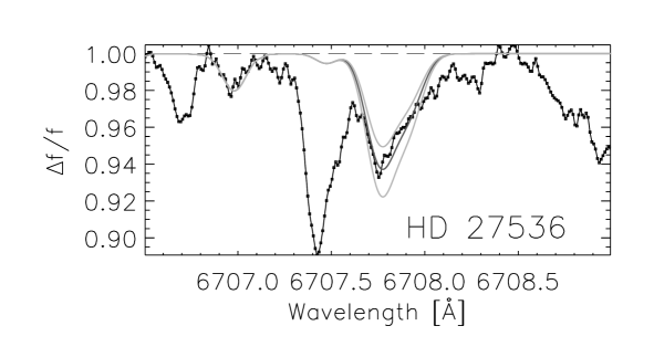
Figure 7: The lithium line region in HD 27536 with fits using three different abundances ($-$10.94, $-$10.84, $-$10.74). Blending with Fe i and V i, but not with CN, has been taken into account.

The Li lines in the solar spectrum could not be reliably measured, so we are using directly the atomic parameters for the lines. The $gf$ values of the Li lines are among the most accurate for any stellar lines (Smith et al. 1998), and can safely be used in an absolute manner. The result is $A(\mathrm{Li})=-10.84\pm 0.10$ and $-11.19\pm 0.13$ for HD 27536 and HD 216803, respectively, the errors coming primarily from uncertainty in the continuum placement and the influence from the weak Fe i, V i, and CN blends. Identical results are obtained with splot and VWA.

The contribution from CN to the total EW has not been taken into account, since we cannot establish reliable carbon and nitrogen abundances. Only the two C i $\lambda\lambda\,5052.167,5380.337$ Å lines can be measured, and they give deviating results. Assuming [C/Fe] = 0 at most, we expect a contribution from CN of up to a few mÅ, resulting in a possible overestimation of the lithium abundance by 0.1-0.2 dex.

The $\alpha$-elements

The abundances of the electron donor elements Ca, Si and Ti merit separate comments. In active stars these elements are often enhanced with respect to iron (e.g. Morel et al. 2003), hence the enhanced opacity due the H^- absorption need to be accounted for in the model calculations.

While [Si/Fe] and [Ti/Fe] generally agree between Methods 1 and 2, there is some discrepancy concerning calcium for HD 216803, possibly due to the abundance using Method 2 being based on only three lines. Taking an unweighted mean of [Si/Fe], [Ti/Fe] and [Ca/Fe] for HD 27536 we get [$\alpha$/Fe] = $+$0.06 ($+$0.03) from Method 1 (Method 2). Excluding calcium, we find similarly [$\alpha$/Fe] = $+$0.05 ($+$0.03) for HD 216803. Within the uncertainties, this result is compatible with no $\alpha$-enhancement for both stars, and we did indeed use [$\alpha$/Fe] = 0.0 in the model calculations.

Chromium

Using Method 1 three Cr i and three Cr ii lines were used for HD 27536. The Cr i lines yielded $+$0.13 with a spread of only 0.01 dex while the Cr ii lines gave $+$0.05, again with a spread of only 0.01 dex. Assuming this difference to be real and not just a statistical effect, we believe the difference to be due to shortcomings of the model atmosphere, rather than reflecting errors in $\log g$.

Vanadium

For both stars we find very high abundances of vanadium ([V/Fe]) using either method. Rather than a true overabundance, this may actually reflect temperature inhomogeneities on the stellar surface, indicating substantial spot coverage (e.g. Gray & Johanson 1991; Strassmeier & Schordan 2000). Vanadium lines are known to be strongly enhanced in sunspots (Wallace et al. 1999) since they have a very strong temperature dependence. Alternatively, the cause may be NLTE effects, but we do not find any trends of abundance versus EW, which would indicate this.

4.3 Line list comparisons

Several studies of stellar atmospheric abundances have employed different line lists, all carefully crafted to suit the analysis for which they are intended and this work is no exception. Our line list is selected directly from the VALD database based on the quality of the spectrum under investigation, i.e. the list will depend on the S/N of the spectrum and the amount of blending, and hence be a function of spectral type and rotational velocity. We have tested two different selection schemes: (1) From the full line list we select manually the best non-blended lines from a comparison with the spectrum under investigation, and (2) we use the full VALD line list and subsequently reject outlying abundance values.

The two schemes yield very similar results when used to find the stellar parameters for HD 27536. In scheme 2 we use 346 Fe i and 31 Fe ii lines after rejection iteration, while for scheme 1 we selected 205 Fe i and 15 Fe ii lines. The differences in atmospheric parameters for HD 27536 are $\Delta T_{\mathrm{eff}}=10$ K, $\Delta\log g=0.00$, $\Delta\xi_{t}=0.1$ km s^-1 between the two line lists. In Figs. 2 and 8 we show the diagnostic plots of the two different line lists, both using Method 1 for the analysis. The derived abundances differ by 0.02 dex at most, with most elements differing less than 0.01 dex. Hence we can conclude that using all possible lines, relying on the statistical accuracy of a sufficiently large number of lines works as well as a manually selected set of lines.

Figure 8: Same as Fig. 2, but using the manually selected line list.

While the two methods prove to be internally consistent, we had some concern about how they compare with each other. In Fig. 9 we show the EWs measured using DAOSPEC (EW₁) versus the EWs of the same lines using VWA (EW₂), and as can be seen, there is a systematic offset between the EWs of the two methods.

Figure 9: The EWs as measured for 110 Fe i lines using DAOSPEC (EW₁) and VWA (EW₂). The dashed line is the EW₁ = EW₂ relation. As can be seen, DAOSPEC EWs are systematically lower than the synthesized.

In order to investigate the effects this offset may have on the model parameters, we calculated the abundances using the VWA EWs with Method 1. In Fig. 10 we show the Fe diagnostic plot for the VWA EWs with the model found by Method 1.

Figure 10: Iron diagnostic plot using the EWs found by Method 2 with the model found by Method 1. See Fig. 2 for legend.

As can be seen, the agreement is excellent, and also the abundances are all the same within 0.02 dex, which means that either method of EW calculation leads to the same fundamental model parameters and the same abundances — provided they are properly calibrated on the spectrum of the Sun. We refer the interested reader to the DAOSPEC manual for an excellent discussion of continuum fitting and the problems involved.

We necessarily also calculated the absolute iron abundance of the Sun, again using Method 2 EWs with Method 1; the results of which is $A(\mathrm{Fe})_{\odot}=-4.47\pm 0.13$, while using the DAOSPEC EWs we find $A(\mathrm{Fe})_{\odot}=-4.53\pm 0.14$, using exactly the same set of Fe i lines. The solar iron abundance from Grevesse & Sauval (1998) is $A(\mathrm{Fe})_{\odot}=-4.54$, hence it is not possible from this result to determine which EW determination is the most correct (if indeed such a concept is meaningful), since both methods give consistent results within the errors.

4.4 Radial velocities, bisectors and activity indexes

The activity indexes for HD 27536 and HD 216803 are listed in Table 2. The main error source is the errors on $V-R$, while the error from measuring the fluxes in the spectra are around $0.02$ on $\log R_{\mathrm{HK}}$ for both stars. Strassmeier et al. (1990) found $\log R_{\mathrm{HK}}=-3.85$ for HD 27536. Taking into account the differences in derived $T_{\mathrm{eff}}$ and $V-R$, the present result and the findings of Strassmeier et al. (1990) are similar: using their parameters, our values of $\log R_{\mathrm{HK}}$ would shift by $+0.21$.

For HD 27536 we have acquired six RV measurements with irregular intervals (see Table 1). These are shown in Fig. 11 along with an orbital fit using the known 306.9 d photometric period. While the measurements are consistent with the period, it is clear that more measurements are needed. To investigate whether this variation may be due to a low-mass companion, we measured the line bisectors using the procedure of Queloz et al. (2001). We measured the bisector inverse slope (BIS) of the mean CCF of the spectra, and compared with the measured RV to check for correlations (Fig. 12, upper panel). As can be seen there seem to be a correlation between the two quantities, indicating that the variation is internal to the star, probably due to activity i.e. spots moving across the stellar disk. Another indication of this comes from the activity index $R_{\mathrm{HK}}$, which is shown in the middle panel of Fig. 12 as a function of RV. This shows exactly the same behavior as the BIS, strenghtening the interpretation that the RV variation is due to activity variations. The correlation between the photospheric variation (BIS) and chromospheric ($R_{\mathrm{HK}}$) activity seem to be very strict (Fig. 12, lower panel), in accordance with expectations (e.g. Messina et al. 2001).

Obviously, part of the variation may be due to an unseen companion, hiding in the activity induced jitter. Unfortunately, our measurements are too sparse to allow a definite conclusion. It is worth noting that Queloz et al. (2001) found a negative correlation between BIS and RV in the case of HD 166435, which allowed the authors to conclude that the RV variation was induced by activity. On the other hand, we find a positive correlation between BIS and RV, as did Santos et al. (2002) in the case of the visual binary HD 41004, which was ascribed to a brown dwarf orbiting the fainter B component. Later, Zucker et al. (2004) identified the RV signature of a giant planet around the A component. Hence, in the case of HD 27536 we cannot exclude the possibility of companion induced RV, activity and BIS variations, but more observations are evidently needed. Even so, if we assume that the activity is indeed induced by an orbiting companion interacting magnetically with the star, we would expect a RV “jitter” of 10–20 m s^-1 based on the calibrations of Santos et al. (2000), i.e. consistent with the observed variation, although their calibration strictly speaking only is valid for dwarfs. To disentangle any companion-induced pull from the activity jitter would thus require several years of monitoring, since the period is so long and since the orbital pull and the induced activity may have the same period. Assuming the period of the hypothetical companion to be equal to the photometric period of 306.9 d, and adopting an inclination of $90^{\circ}$, we find a mass of $\sim 3.9$ M_J orbiting in an eccentric ($\epsilon\sim 0.5$) orbit with semi-major axis $\sim 1.2$ AU. This is under the assumption that all the RV variation is due to an unseen companion. More likely, a companion would induce a smaller effect on top of the (larger) activity induced jitter. Note also, that the photometric variation is sinusoidal, as shown by Strassmeier et al. (1999), which is hard to reconcile with the eccentric “orbit” suggested by the RV data.

Figure 11: RV variations measured in HD 27536. The variation is consistent with the known 306.9 day period, but obviously long-term monitoring is necessary. The dotted curve is a binary orbit fit with the known photometric period.

Figure 12: Upper panel: Line bisector inverse slope (BIS; see text for definitions) vs RV. Middle panel: Activity index $\log R_{\mathrm{HK}}$ versus RV. Lower panel: $\log R_{\mathrm{HK}}$ versus BIS. There seem to be a clear correlation between activity level and RV, and between the BIS and the activity, pointing to changing activity as the cause of the RV variations. The error-bars on $\log R_{\mathrm{HK}}$ are only measurement errors i.e., not including uncertainties in $V-R$ and T_eff, since these would affect all measurements equally.

5 Conclusions

In this paper we have presented a pilot study of active stars, presenting and discussing the tools to be used on a larger sample.

We have presented results on the two photometrically variable, late-type active stars HD 27536 and HD 216803, deriving their fundamental atmospheric parameters and photospheric elemental abundances from high-resolution spectra. We accomplished this task using two different methods, which produced results in good agreement with each other, giving credibility to the derived parameters and abundances. Furthermore, we have showed that, despite the obvious differences in derived EW between the two methods, and despite the differences in line lists employed, we derive essentially the same results. Both methods have a GUI, which greatly increases user-friendliness. Especially Method 1 has been developed with a view to automation, and the ultimate goal is to be able to determine atmospheric parameters and abundances for a great number of spectra without any human intervention.

While the agreement between the two methods is very tight for HD 27536, larger differences resulted for HD 216803 ($\Delta$[M/H]$\sim 0.06$). Even so, the abundances relative to iron, i.e. [M/Fe], show near perfect agreement between the two methods, except for calcium, which may be due to poor statistics.

Our study demonstrates the importance of determining relative abundances with respect to the Sun, which minimizes any errors introduced by uncertain $gf$ values and uncertainties in continuum treatment. On the other hand, the presence of surface spots may influence the determination of $\log g$ through the ion balance, wherefore it may be better to use different approaches, or select lines based on their sensitivity to spots.

Due to the high intrinsic stability of the HARPS spectrograph, a detailed analysis of the RV and bisector variations was possible, using the limited data set of HD 27536. We find a RV variation, which is consistent with the known photometric period, although our coverage is not long enough to judge whether this is indeed the true period, or if the variations are periodic at all. We find a remarkable correlation between the bisector inverse slope and the activity index $\log R_{\mathrm{HK}}$, which both vary in phase with the RV, revealing a very tight correlation between the photospheric and chromospheric activity. The fact that we find a positive correlation may hint at the existence of an unseen companion, but our phase coverage is not yet good enough to explore this possibility.