The blueshift of the [O III] emission line in NLS1s

Abstract

We investigate the radial velocity difference between the narrow emission-line components of [O III] $\lambda$ 5007 and H$\beta$ in a sample of 150 SDSS NLS1s. Seven “blue outliers” with [O III] blueshifted by more than 250 km s^-1are found. A strong correlation between the [O III] blueshift and the Eddington ratio is found for these seven “blue outliers”. For the entire sample, we found a modest correlation between the blueshift and the linewidth of the narrow component of the [O III] line. The reflected profile of [O III] indicates two kinematically and physically distinct regions. The [O III] linewidth depends not only on the bulge stellar gravitational potential, but also on the central black hole potential.

1 INTRODUCTION

As an interesting subclass of active galactic nuclei (AGNs), narrow-line Seyfert 1 galaxies (NLS1s) were initially defined with the following optical spectral characteristics: H$\beta$ full width half maximum (FWHM) less than $2000$ km s^-1; strong optical Fe II multiplets; a line-intensity ratio of [O III]$\lambda$5007 to H$\beta$ less than 3, which distinguishes between Seyfert 1 and Seyfert 2 galaxies (Osterbrock & Pogge 1985; Goodrich 1998). A steep, soft X-ray excess (Puchnarewicz et al. 1992; Boller et al. 1996) and rapid soft/hard X-ray variability (Leighly 1999; Cheng et al. 2002) are shown in the X-ray observations of NLS1s. The popular model of NLS1s is that they contain less massive black holes with higher Eddington ratios (Pounds et al. 1995; Wandel & Boller (1998); Laor et al. 1997; Mineshige et al. 2000), suggesting that NLS1s might be in the early stage of AGN evolution (Grupe 1996; Mathur 2000; Bian & Zhao 2003).

Based on the standard model of AGNs, the characteristic emission lines are emitted from the so-called broad line region (BLR) and the narrow line region (NLR) (see Sulentic et al. 2000 for a review of the BLR). The reverberation mapping technique shows that the kinematics of the emitting gas in the BLR are determined by the gravitational potential of the central supermassive black hole (Peterson & Wandel 2000). The correlation between the bulge stellar velocity dispersion (derived from Ca II absorption and [O III] emission) suggests that the NLR kinematics are determined, in large part, by the bulge potential (Nelson & White 1996). Therefore, the FWHM of the [O III] line may be adopted as a surrogate of the bulge stellar velocity dispersion. Recently, using the Sloan Digital Sky Survey (SDSS), we find that NLS1s as a class deviate from the $M_{\rm BH}-\sigma$ relation seen in normal galaxies. This is confirmed by other investigations with ROSAT data, and it is suggested that the black holes with higher Eddington ratios in some NLS1s are still growing (Grupe & Mathur 2004; Mathur & Grupe 2005). Although Boroson (2003) suggested that for AGNs the stellar velocity dispersions measured by [O III] can predict the black hole mass to a factor of five, it is possible that the [O III] width is not a good tracer of the velocity dispersion for NLS1s. Botte et al. (2005) find that the [O III] linewidth indeed typically overestimates the stellar velocity dispersion compared to the direct measure of the Ca II absorption triplet. These results support that the dynamics of the NLR in NLS1s would be different than that of other AGNs.

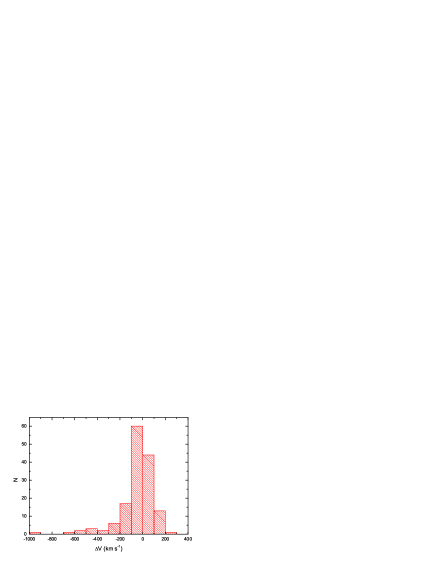
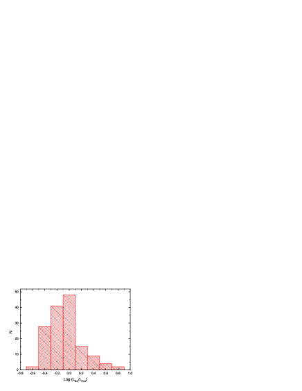
Figure 1: The distribution of the [O III] blueshift relative to H$\beta$ ($\Delta~{}V$) in units of km s^-1(left) and the distribution of $L_{bol}/l_{Edd}$ (right) for SDSS NLS1s.

Outflows have been reported in some NLS1s. A very significant blueshift of about $10\AA$ for the [O III] line relative to the rest-frame defined by the H$\beta$ line is found in the prototype NLS1 I ZW 1 (Boroson & Oke 1987). This kind of blueshift is generally interpreted as the NLRs outflow relative to the BLRs. Zamanov et al. (2002) also find other six AGNs showing the [O III] blueshifts larger than 250 km s^-1in their sample of 216 type 1 AGNs (Marziani et al. 2003a), and these objects are called “blue outliers”. Two NLS1s with the largest [O III] blueshifts were recently found by Aoki, Kawaguchi & Ohta (2005). Up to now, 16 “blue outliers” have been found (Grupe 2001; Verron-Cetty et al. 2001; Grupe & Leighly 2002; Zamanov et al. 2002; Marziani et al. 2003b; Aoki, Kawaguchi & Ohta 2005). The distribution of these “blue outliers” in the eigenvector 1 diagrams is found to be in the population A region of the Eigenvector 1 parameter domain (see Fig. 1c in Zamanov et al. 2002). The “blue outlier” is the population with strong Fe II lines and narrow H$\beta$ line, very similar to the characteristics of NLS1s.

In this paper, we use the SDSS NLS1s to find more “blue outliers”. For the “blue outliers” in our sample, we carefully model the emission lines of H$\beta$ and [O III] with multiple components, which will provide some clues about the NLR dynamics of the “blue outliers”. All of the cosmological calculations in this paper assume $H_{0}=75\rm{~{}km~{}s^{-1}~{}Mpc^{-1}}$, $\Omega_{M}=0.3$, $\Omega_{\Lambda}=0.7$.

2 SAMPLE AND ANALYSIS

Using the NLS1 selection criteria outlined above (Osterbrock & Pogge 1985; Goodrich 1989), Williams et al. (2003) generated a sample of 150 NLS1s found within the SDSS Early Data Release (EDR), which is the largest published sample of NLS1s. The spectra of these 150 NLS1s are obtained from SDSS Data Release 3 (DR3). Because of the lack of the [O III] line, SDSS J153243.67-004342.5 is ignored in our analysis.

The spectra are transformed into the rest frame defined by the redshift given in their FITS header. Because of the asymmetry of the profiles of [O III] and/or H$\beta$ lines, we used two-component models to fit the emission lines of H$\beta$ and [O III] $\lambda\lambda$4959, 5007, employing the IRAF task SPECFIT (Kriss 1994) for a careful look at the [O III] blueshift phenomenon (e.g. Zheng et al. 2002; Dong et al. 2005). The Galactic interstellar reddening was corrected using E(B-V)=0.046 (Schlegel et al. 1998), assuming an extinction curve with $R_{V}=3.1$.

NLS1s generally show strong Fe II emission lines which contaminate the continuum and the emission lines of H$\beta$ and [O III]$\lambda\lambda$4959,5007. The Fe II template, derived from the prototype NLS1 I ZW 1 (Boroson & Green 1992), is used to subtract the Fe II multiples from the spectra. It is broadened by convolving with a Gaussian of various line widths and scaled by multiplying by a factor indicating the line strength. At the same time, a power-law continuum is also fit. The best Fe II and power-law subtraction is found when the spectral regions between the H$\gamma$ and H$\beta$ (Fe II multiplets 37, 38) and between 5100Åand 5400Å(Fe II multiplets 48, 49) are flat.

We use two Gaussians to model the line profiles of [O III] and H$\beta$. For the doublet [O III] $\lambda\lambda$4959,5007, we take the same linewidth for each component, and fix the flux ratio of [O III]$\lambda$4959 to [O III]$\lambda$5007 to be 1:3.

We measure the wavelength difference between the centroid of the narrow components of H$\beta\lambda$4861.3 and [O III]$\lambda$5006.8 lines (i.e. the peaks of the H$\beta$ and [O III] lines). Then the [O III] blueshift relative to H$\beta$ (i.e. $\Delta V$) in units of km s^-1can be calculated based on the the laboratory wavelength difference (145.5Å). In order to investigate the drivers of the [O III] blueshift, we also calculated the Eddington ratio, i.e. the bolometric luminosity as a fraction of the Eddington luminosity ($L_{bol}/L_{Edd}$). We take $L_{bol}=9\lambda L_{\lambda}(5100\AA)$ (Kaspi et al. 2000) and $L_{Edd}=1.26\times 10^{38}M_{bh}/\mbox{\,$\rm M_{\odot}$}~{}ergs~{}s^{-1}$, where $M_{bh}$ is the black hole mass. $\lambda L_{\lambda}(5100\AA)$ is derived from the r^∗ magnitude. $M_{bh}$ is calculated from H$\beta$ FWHM and the empirical size-luminosity formula (Kaspi et al. 2000). $\lambda L_{\lambda}(5100\AA)$ and $M_{bh}$ values are respectively taken from Col.4 and Col.5 in Table 1 of Bian & Zhao (2004a). The best-fit Fe II flux between 4434$\AA$ and 4684$\AA$ is calculated from Fe II spectra and the flux ratio of the Fe II (between 4434 and 4684Å) to H$\beta$ (Fe II$\lambda$ 4570/H$\beta$) is also calculated.

Following Zamanov et al. (2002), we take $\Delta V<-250$ km s^-1as the criterion for classification as a “blue outlier” and finally select the blue outliers in the sample of SDSS NLS1s.

3 RESULTS

3.1 Distributions of the blueshift and the Eddington ratio

Fig. 1 shows the distribution of the derived [O III] blueshifts for these 149 NLS1s. The mean value of the [O III] blueshift is $-52\pm 13$ km s^-1with a standard deviation of 158 km s^-1.

It is generally accepted that the Eddington ratio is large in NLS1s, which is possibly related to the outflow phenomena. Fig. 1 also shows the distribution of the Eddington ratios in the logarithm. The mean value is $-0.06\pm 0.02$ with a standard deviation of 0.26. Many NLS1s have relatively small Eddington ratios. Considering the correlation between the X-ray spectral index and the Eddington ratio (Grupe 2004; Bian 2005), these objects with lower Eddington ratios should not have very steep X-ray photo indices, which is consistent with recent Chandra observations of some SDSS NLS1s (Williams, Mathur & Pogge 2004).

3.2 Correlations between the blueshift and other parameters

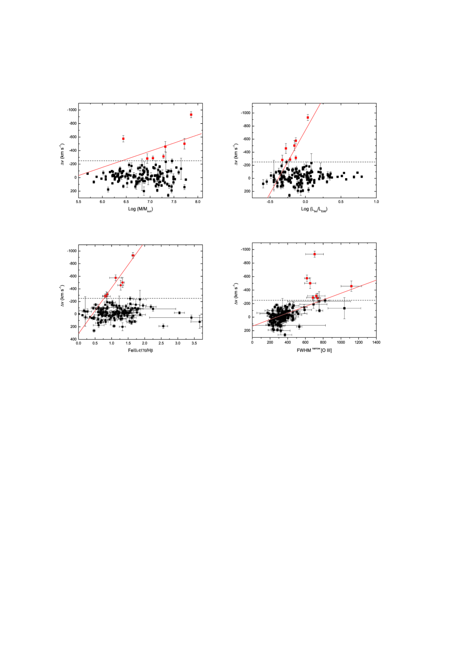
Figure 2: The [O III] blueshift versus $M_{bh}$, $L_{bol}/l_{Edd}$, $FeII\lambda 4570/H\beta$, and $FWHM^{narrow}([OIII])$. The red squares denote the “blue outliers”. The dash line shows -250 km s^-1. The red solid lines in the figures of $\Delta-M_{bh},L_{bol}/l_{Edd},FeII\lambda 4570/H\beta$ are our best fit for seven “blue outliers.” The red solid lines in the figure of $\Delta-FWHM^{narrow}([OIII])$ is the best fit for all 149 SDSS NLS1s.

In Fig. 2, we show the [O III] blueshift as a function of the black hole mass, the Eddington ratio, and Fe II $\lambda$4570/H$\beta$. Using the simple least square linear regression (Press et al. 1992), no significant correlations are found. We also plot in Fig. 2 the [O III] blueshift versus FWHM of the narrow component of the [O III] line. The simple least square linear regression shows a modest correlation with a correlation coefficient is 0.54. NLS1s with larger [O III] blueshift tend to show broader [O III] linewidth.

3.3 The “blue outliers”

Although the spectra have low signal-to-noise ratios, larger displacements in some NLS1s exist in both [O III]$\lambda$4959 and [O III]$\lambda$5007 relative to the rest frame defined by the narrow component of H$\beta$ line. The errors and uncertainties are discussed in Sec. 4.1.

Taking $\Delta V<-250$ km s^-1as our criterion (Zamanov et al. 2002), we found 13 NLS1s to be “blue outliers.” For some NLS1s with low signal-to-noise spectra, the wavelength error of the line centroid (for the narrow/broad components of H$\beta$/[O III] lines) in the fitting is sometimes large. Because the line centroid error of some component is larger than 5$\AA$, we consider six objects in these 13 NLS1s to be questionable classifications. At last we obtain seven reliable “blue outliers.” The parameters of these seven “blue outliers” are listed in Table 1. Considering the lower limit of the blueshift, one NLS1 does not satisfy the criterion of $\Delta V<-250$ km s^-1, and that is SDSS J115533.50+010730.6.

In Fig. 2, red squares denote the seven reliable “blue outliers”. Using the simple least square linear regression (Press et al. 1992), correlations between the [O III] blueshift and the black hole mass, the Eddington ratio, Fe II $\lambda$4570/H$\beta$ are found and the correlation coefficients are listed in Table 2. “Blue outliers” tend to show broad [O III] linewidth.

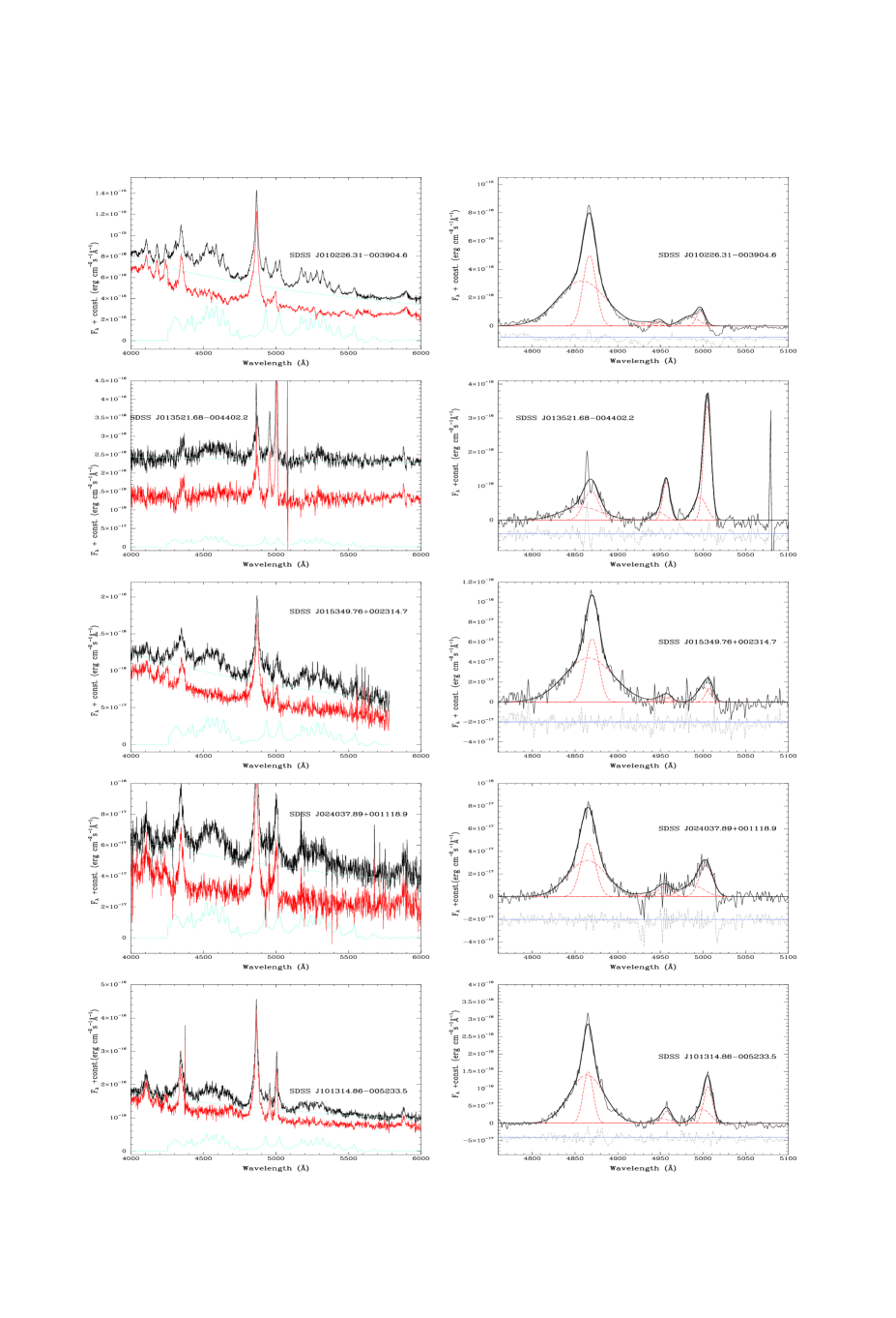
Figure 3: Rest-frame spectra of “blue outliers” (left): the observed spectrum and a power-law continuum (top curve), Fe II-subtracted spectrum (middle curve), and Fe II spectrum (buttom curve); Multi-component fitting of the H$\beta$ and [O III]$\lambda\lambda$4959, 5007 (right): modeled composite profile (thick solid line), individual components (the dotted lines), the residual spectrum (lower panel).

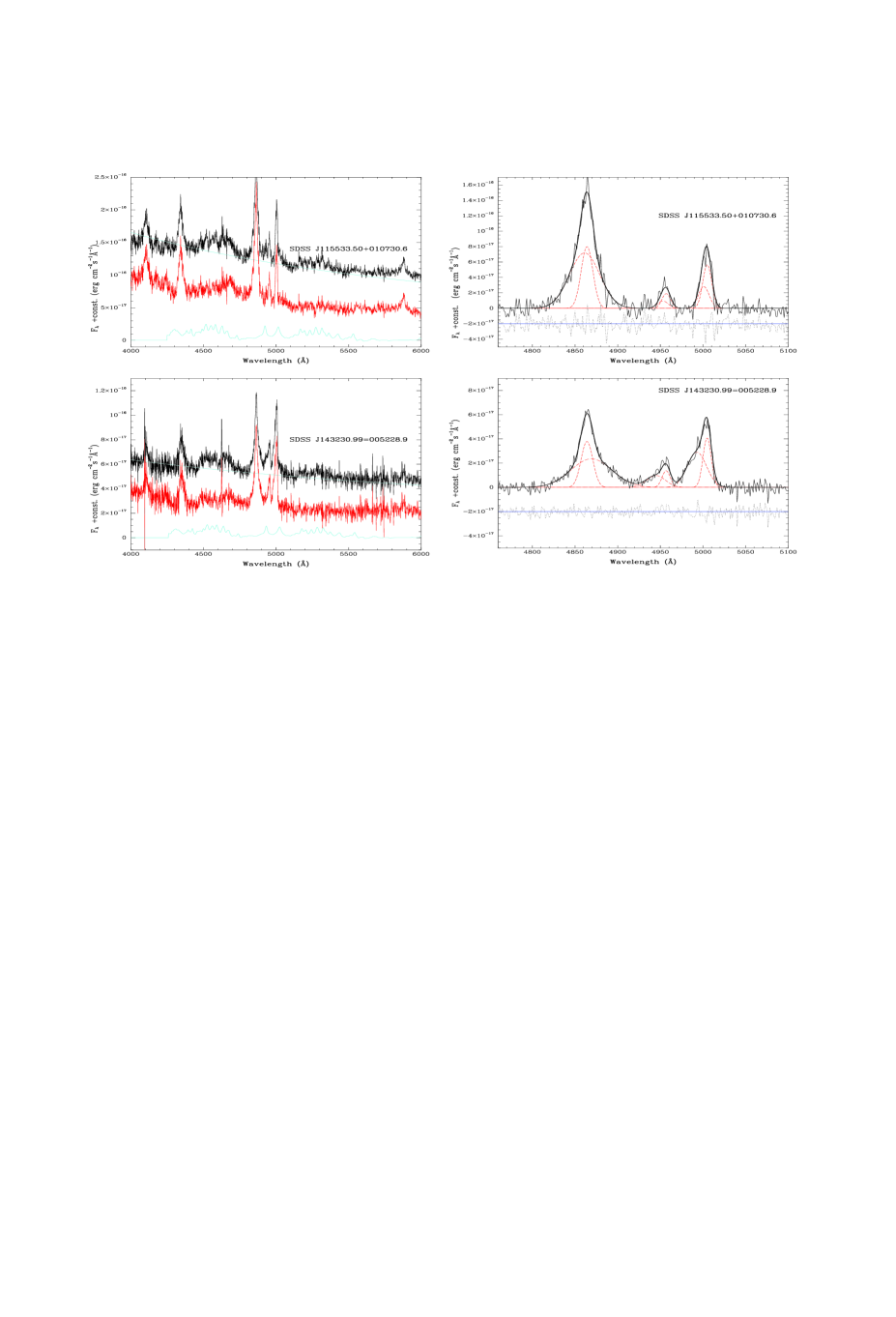
Figure 3: Continued.

Fig. 3 shows rest-frame spectra for the “blue outliers” (left). The Fe II spectra are shown in the bottom in each left panel. Remarkable Fe II emission is obvious. The value of Fe II$\lambda$ 4570/H$\beta$ is listed in Col. 9 in Table 1. We also plot two-component fitting of H$\beta$ and [O III]$\lambda\lambda$4959, 5007 (right) in Fig. 3. The fitting depends on the spectra quality. The fitting goodness is illustrated by the residual spectrum shown in the bottom in each right panel. Using different initial-values, the best values and the errors for different line components (e.g. FWHM, the line flux, and the [O III] blueshift relative to the narrow component of H$\beta$) are listed in Table 3 for these “blue outliers”.

4 DISCUSSION

4.1 Errors

We have found obvious differences between the spectra of the same NLS1s released from SDSS EDR and DR3, up to a factor of 1.5 for some NLS1s. This would lead to the uncertainty of 0.1 dex at most in the mass estimate. In Fig. 3 of Bian & Zhao (2004a), we found that monochromatic luminosity at 5100$\AA$ measured from the spectra of the SDSS NLS1s is lower than that derived from $r^{\ast}$ band magnitude by 0.21 in the logarithm scale. The new flux calibration shows that the monochromatic luminosity at 5100$\AA$ measured from the spectra is consistent with that derived from $r^{\ast}$ band magnitude. The optical magnitude (here we adopted the $r^{\ast}$ band magnitude) is popularly used to derive the BLR size and then to calculate the black hole virial mass from the H$\beta$ FWHM (e.g. Wang & Lu, 2001; Gu, Cao & Jiang, 2001; Bian & Zhao 2004a; Bian & Zhao 2004b). Using this method, we can estimate the black hole virial mass within a factor of 3 (i.e., $\sim 0.5$ dex) (Bian & Zhao 2004a, Bian & Zhao 2004b). The error in the Eddington ratio, ($L_{bol}/L_{Edd}$) largely depends on the error in the black hole mass. They are almost the same, i.e. $\sim 0.5$ dex.

The [O III] blueshift relative to H$\beta$ is calculated from their centroid wavelength difference. The error of the [O III] blueshift depends on the errors of the centroid wavelengthes of the [O III] line and H$\beta$ line, and is calculated from propogating their errors, which are shown in Fig. 1. For our “blue outliers”, the errors of the blueshifts are also listed in Table 3. The typical errors of the centroid of the narrow component of the [O III] line and the H$\beta$ line are 1 Å, i. e., 60km s^-1. For the linewidth and the line flux, the typical error is about 10%. However, the systematic effects are neglected, e.g., the uncertainties of the continuum substraction, the Fe II template, and component decomposition (Greene & Ho 2005). The instrumental FWHM is about 60 km s^-1for the [O III] line, which is small relative to the [O III] FWHM. Therefore, the centroid of the narrow components of H$\beta$ and [O III] is reliable.

4.2 Largest [O III] blueshift: SDSS J010226.31-003904.6

The “blue outlier” with the largest [O III] blueshift is SDSS J010226.31-003904.6 (see Table 1). It has the strongest Fe II$\lambda$4570/H$\beta$ as well. Strong Fe II emission lines contaminate its continuum and seriously blend with the lines of H$\beta$ and [O III]$\lambda\lambda$4959,5007. There are two peaks in the region of [O III]$\lambda$5007. One peak is due to Fe II emission (see Fig. 3). After the Fe II template is subtracted, we found that the profile of [O III]$\lambda$5007 is asymmetric and used a two-component fitting (see Fig. 3). Although the spectrum is noisy, we still found that the blueshift of the narrow component of [O III] relative the narrow component of H$\beta$ is $-931\pm 46$ km s^-1. Aoki et al. (2005) also presented this object as one of the two largest blueshifts and they measured the blueshift to be $-880\pm 30$ km s^-1. These two measurements are consistent within their errors. $M_{bh}$ is $10^{7.86}\mbox{\,$\rm M_{\odot}$}$ and $L_{bol}/L_{Edd}$ is 0.034, which are also consistent with the results from Aoki et al. (2005) considering the uncertainties of $\sim 0.5$ dex in $M_{bh}$ and $L_{bol}/L_{Edd}$. Other parameters are listed in the first line in Table 1.

4.3 Drivers of the [O III] blueshift

It is clear that [O III] blueshifts relative to H$\beta$ exist in AGN spectra, especially in NLS1s (see Fig. 3 and Table 3.). The distribution of the [O III] blueshifts is very similar to the result of Zamanov et al. (2002) (see Fig. 1b therein). The origin of the [O III] blueshift relative to H$\beta$ is still a question of debate. The standard model of AGNs is the disk accretion around the central supermassive black hole with the BLR, NLR, and jet. The [O III] blueshift is generally interpreted as an indicator of the outflow in AGNs (e.g. Aoki, et al. 2005). Marziani et al. (2003b) find that “blue outliers” have higher Eddington ratios, and the accretion may be the engine of this outflow.

However, no correlation is found between the [O III] blueshift and the Eddington ratio in another sample of 16 “blue outliers” (Aoki et al. 2005). They suggested that the [O III] blueshift only weakly depends on the Eddington ratio. Here we also showed the relations between the [O III] blueshift and the Eddington ratio, black hole mass in Fig. 2. Although no correlation is found for the entire NLS1 sample, a strong correlation is found for our “blue outliers.” The relationship between the [O III] blueshift and $L_{bol}/L_{Edd}$ is stronger than that between [O III] blueshift and $M_{bh}$ (see Table 2). However, no correlation is found if we combine the Aoki et al. (2005) 16 “blue outliers” and ours together. This is possibly due to the larger uncertainties in the Eddington ratio.

The blueshift of [O III] is possibly the result of the outflowing gas from the nucleus and the obscuration of the receding part of the flow which depends on the viewing angle (Zamanov et al. 2002). The outflowing gas is possibly from the inner NLR, which is related to the wind of the accretion disk and would have larger linewidth (Elvis 2000). The blueshift and larger linewidth of [O III] can be interpreted in this scenario (Zamanov et al. 2002).

Some possible necessary conditions are suggested to produce the outflow (Aoki et al. 2005): larger black hole masses ($>10^{7}\mbox{\,$\rm M_{\odot}$}$), higher accretion rates ($>2\mbox{\,$\rm M_{\odot}$}~{}yr^{-1}$), or larger luminosity ($\lambda L_{\lambda}(5100\AA)>10^{44.6}~{}ergs~{}s^{-1}$) (see Fig. 8 therein). Based on our “blue outliers” found in SDSS sample (see Table 1), the black hole masses in most of our “blue outliers” are larger($>10^{7}\mbox{\,$\rm M_{\odot}$}$). The condition of larger luminosity is not confirmed by our sample.

Aoki et al. (2005) suggested there is a strong correlation between the [O III] blueshift and the radio luminosity for their 16 “blue outliers”. Here we find other six “blue outliers” in SDSS NLS1s. Radio data for these “blue outliers” is needed to check this correlation. For radio-loud NLS1s, we should used the H$\beta$ luminosity instead of $\lambda L_{\lambda}(5100\AA)$ to derive the black hole mass (Wu et al. 2004; Kaspi et al. 2005).

4.4 Dynamics of [O III]

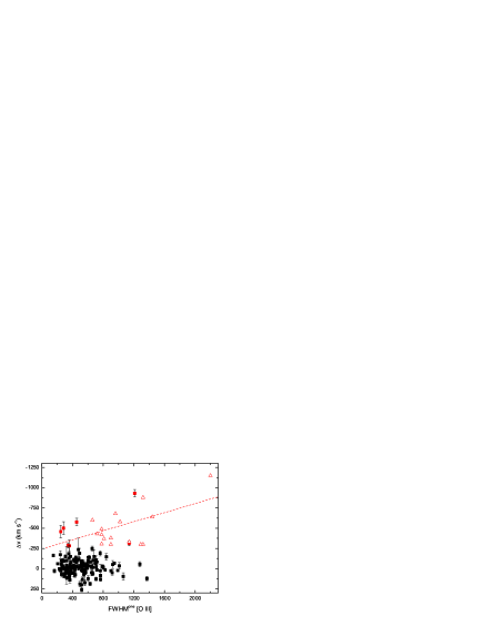
Figure 4: The [O III] blueshift versus $FWHM^{one}([OIII])$. Open triangles denote the “blue outliers” in the sample of Aoki et al. (2005). The red dash line is our best fit for all “blue outliers” from the sample of Aoki et al. (2005) and our SDSS NLS1s sample.

The [O III] FWHM or its narrow/core component can be used as an indicator of the black hole mass (Nelson & Whittle 1996; Greene & Ho 2005). Our “blue outliers” tend to show large [O III] FWHM, which is consistent with the results of Aoki et al. (2005). For all SDSS NLS1s in our sample, the correlation coefficient is -0.55 for the relation between the [O III] blueshift and the FWHM of the narrow component of [O III] line. However, for our “blue outliers,” this relation is very weak. We also used the [O III] FWHM measured with single Gaussian fit ($FWHM^{one}([OIII]$), Col. 6 in Table 1 in Bian & Zhao 2004a). However no correlation is found between the [O III] blueshift and $FWHM^{one}([OIII])$ for all SDSS NLS1s or the “blue outliers”. Combining the Aoki et al. 16 “blue outliers” and our “blue outliers” together, a modest correlation is found between the [O III] blueshift and $FWHM^{one}([OIII])$ is found (R=0.54, P=0.007, Fig. 4).

The two components of the [O III]$\lambda\lambda$ 4959, 5007 lines are found to have different linewidths and blueshifts relative to the narrow H$\beta$ line. We interpret these two components as two kinematically and physically distinct regions in this blue outlier (Holt, Tadhunter & Morganti, 2003). The broad component of [O III]$\lambda$5007 is almost the same order of magnitude as expected for the BLR. This is consistent with the above outflow/wind scenario for the inner NLR, which is influenced by the central black hole potential. Therefore, the [O III] complex indicates that its width depends not only on the bulge stellar gravitational potential, but also on the central black hole potential.

Verron-Cetty (2001) suggests that Lorentzian profiles rather than Gaussians are more suitable to reproduce the shape of NLS1 broad emission lines. Considering the low signal-to-noise ratio of the SDSS NLS1 spectra, we found Gaussian profiles work fine. It is normally expected that the line ratio of [O III]$\lambda$5007 to H$\beta$ is about 10, and such a blueshift of the narrow component of H$\beta$ line from NLRs will be lost in the noise. Rodriguez-Ardila et al. (2000) suggested that the [O III]$\lambda$5007/H$\beta$ ratio emitted in NLR varies from 1 to 5, instead of the normally expected value of 10. If that is the case, we should use FWHM of the broad component of H$\beta$ to calculate the black hole mass, and we should pay more attention to our black hole mass estimate and the Eddington ratio. We found that the NLR contribution needs to subtracted to calculate the black hole mass correctly, especially for objects with larger [O III] flux. This will presented in our next paper. For our “blue outliers,” the [O III] flux is relatively weak. Therefore, as far as the H$\beta$ emission line is concerned, the contribution from NLR in these “blue outliers” can be neglected.

5 CONCLUSIONS

The blueshift of the narrow component of [O III] relative to the narrow component of H$\beta$ is investigated for a sample of 150 SDSS NLS1s. The main conclusions can be summarized as follows.

• We have measured the radial velocity difference between the narrow components of [O III] $\lambda$5007 and H$\beta$ lines for 149 SDSS NLS1s. The mean value of the [O III] blueshift relative to H$\beta$ is $-52\pm 13$ km s^-1with a standard deviation of 158 km s^-1.

• We have found seven “blue outliers” ($\sim 5\%$ in the SDSS NLS1 sample) if taking $250km~{}s^{-1}$ (i.e. about 4Å) as the criterion of the “blue outlier.” Considering one lower limit, six NLS1s satisfied this criterion. The “blue outliers” with the largest [O III] blueshift is SDSS J010226.31-003904.6 with a measurement of $-931\pm 46$, which is consistent with the results of Aoki et al. (2005).

• Strong correlations are found between the amount of the [O III] blueshift and the Eddington ratio, and Fe II $\lambda 4570$/H$\beta$, which supports the outflow/wind scenario as the origin of the [O III] blueshift. The correlation of $\Delta V-L_{bol}/L_{Edd}$ is stronger than the correlation of $\Delta V-M_{bh}$. For the whole sample of 149 NLS1s, we also found a modest correlation between the [O III] blueshift and FWHM of the narrow component of the [O III] line.

Name	z	FWHM of H$\beta$	FWHM of [O III]	$\lambda L_{\lambda}$	$logM_{bh}$	$logL_{bol}/L_{Edd}$	$\Delta V($km s-1$)$	FeII/H$\beta$
(1)	(2)	(3)	(4)	(5)	(6)	(7)	(8)	(9)
SDSS J010226.31-003904.6	0.294	1680 $\pm$ 60	647$\pm$120	45.04	7.86	0.03387	-931 $\pm$ 46	1.646 $\pm$ 0.037
SDSS J013521.68-004402.2	0.098	1181$\pm$ 182	711$\pm$85	43.45	6.44	-0.13613	-576 $\pm$ 47	1.123 $\pm$ 0.185
SDSS J015249.76+002314.7	0.589	1852$\pm$110	1277$\pm$165	44.71	7.72	-0.15613	-501 $\pm$ 78	1.333 $\pm$ 0.054
SDSS J024037.89+001118.9	0.47	1789$\pm$115	381$\pm$ 70	44.19	7.32	-0.27613	-458 $\pm$ 78	1.276 $\pm$ 0.092
SDSS J101314.86-005233.5	0.276	1578$\pm$ 87	991$\pm$115	44.29	7.28	-0.13613	-314 $\pm$ 31	0.866 $\pm$ 0.039
SDSS J115533.50+010730.6	0.197	1628$\pm$202	919$\pm$85	43.76	6.94	-0.32613	-283 $\pm$ 71	0.844 $\pm$0.12
SDSS J143230.99-005228.9	0.362	1559$\pm$121	1222$\pm$92	43.99	7.06	-0.21613	-288 $\pm$ 31	0.802 $\pm$ 0.07

Table 1: Seven “blue outliers” found in our sample of 150 SDSS NLS1s. Columns are: (1) name; (2) redshift; (3) FWHM of H$\beta$ (one gaussian fitting, Williams, Pogge & Mathur, 2002); (4) the [O III] FWHM (one-Gaussian fitting, Bian & Zhao 2004a); (5) log of continuum luminosity at the rest wavelength 5100 Å in unit of $ergs^{-1}$; (6) log of the black hole mass in units of solar mass; (7) the Eddington ratio; (8) the [O III] blueshift relative to the narrow component of H$\beta$ in units of km s^-1; (9) the flux ratio of the Fe II (between 4434 and 4684 Å) to H$\beta$.

X	R	SD	P	a	b
(1)	(2)	(3)	(4)	(5)	(6)
$LogM_{bh}$	-0.43	5.02	0.33	$1288.4\pm 306.2$	$-240.2\pm 42.5$
$LogL_{bol}/L_{Edd}$	-0.81	3.40	0.03	$-736.7\pm 33.0$	$-1937.6\pm 183.9$
$FeII\lambda 4570/H\beta$	-0.96	1.53	$<10^{-4}$	$308.0\pm 61.8$	$-726.7\pm 58.0$
$FWHM^{narrow}[OIII]$ ∗	-0.55	3.76	$<10^{-4}$	$133.1\pm 5.5$	$-0.50\pm 0.02$

Table 2: Correlations between the blueshift and some parameters for our “blue outliers”. ^∗ shows that it is done for all SDSS NLS1s. Col. 1: other parameters; Col. 2: correlation coefficient; Col. 3: standard deviation; Col. 4: probability that the correlation is caused by a random factor; Col. 5, 6: a and b in $\Delta V$=a+bX.

Line	Component	Rest Wavelength	Velocity shift	FWHM	Line flux
		($\AA$)	(km s-1)	(km s-1)	($10^{-16}ergs^{-1}cm^{-2}$)
(1)	(2)	(3)	(4)	(5)	(6)
SDSS J010226.31-003904.6
H$\beta$	n	$4861.3\pm$ 0.2	0	$1111\pm 46$	$95.6\pm 5.0$
	b	$4852.2\pm$ 0.6	$-559\pm 39$	$4087\pm 97$	$224.4\pm 5.2$
[O III]$\lambda$4959	n	$4943.4\pm$ 0.7	$-944\pm 46$	$703\pm 101$	$4.3\pm 1.1$
	b	$4930.2\pm$ 2.4	$-1742\pm 146$	$1502\pm 176$	$6.0\pm 3.3$
[O III]$\lambda$5007	n	$4991.3\pm$ 0.7	$-931\pm 46$	$703\pm 101$	$12.9\pm 3.3$
	b	$4977.9\pm$ 2.4	$-1730\pm 146$	$1502\pm 176$	$18.0\pm 9.9$
SDSS J013521.68-004402.2
H$\beta$	n	$4861.3\pm$ 0.8	0	$1269\pm 162$	$19.0\pm 4.1$
	b	$4848.9\pm$ 4.4	$-766\pm 277$	$3413\pm 403$	$22.9\pm 4.3$
[O III]$\lambda$4959	n	$4949.3\pm$ 0.2	$-578\pm 47$	$617\pm 28$	$12.3\pm 1.1$
	b	$4940.6\pm$ 1.9	$-1104\pm 125$	$1082\pm 142$	$4.3\pm 1.0$
[O III]$\lambda$5007	n	$4997.2\pm$ 0.2	$-576\pm 47$	$617\pm 28$	$37.0\pm 3.3$
	b	$4988.4\pm$ 1.9	$-1087\pm 125$	$1082\pm 143$	$12.9\pm 3.0$
SDSS J015249.76+002314.7
H$\beta$	n	$4861.3\pm$ 0.3	0	$1128\pm 75$	$12.4\pm 1.2$
	b	$4857.1\pm$ 0.8	$-258\pm 55$	$4177\pm 182$	$31.8\pm 1.1$
[O III]$\lambda$4959	n	$4950.5\pm$ 1.3	$-503\pm 78$	$653\pm 63$	$0.5\pm 0.4$
	b	$4943.1\pm$ 3.5	$-953\pm 211$	$1076\pm 195$	$1.0\pm 0.4$
[O III]$\lambda$5007	n	$4998.4\pm$ 1.3	$-501\pm 78$	$653\pm 63$	$1.6\pm 1.2$
	b	$4990.9\pm$ 3.5	$-936\pm 211$	$1076\pm 195$	$2.9\pm 1.2$
SDSS J024037.89+001118.9
H$\beta$	n	$4861.3\pm$ 0.4	0	$1252\pm 91$	$10.2\pm 1.5$
	b	$4860.3\pm$ 0.9	$-64\pm 59$	$3270\pm 204$	$18.1\pm 1.4$
[O III]$\lambda$4959	n	$4951.2\pm$ 1.2	$-465\pm 78$	$1118\pm 116$	$1.8\pm 0.4$
	b	$4935.7\pm$ 4.6	$-1404\pm 277$	$1867\pm 400$	$1.1\pm 0.4$
[O III]$\lambda$5007	n	$4999.2\pm$ 1.2	$-458\pm 78$	$1118\pm 116$	$5.5\pm 1.2$
	b	$4983.5\pm$ 4.6	$-1390\pm 277$	$1867\pm 400$	$3.3\pm 1.2$
SDSS J101314.86-005233.5
H$\beta$	n	$4861.3\pm$ 0.3	0	$856\pm 67$	$22.0\pm 2.4$
	b	$4859.6\pm$ 0.4	$-104\pm 31$	$2976\pm 100$	$71.6\pm 2.4$
[O III]$\lambda$4959	n	$4953.6\pm$ 0.4	$-321\pm 31$	$723\pm 100$	$4.5\pm 1.6$
	b	$4947.0\pm$ 4.2	$-720\pm 253$	$1313\pm 211$	$3.2\pm 1.7$
[O III]$\lambda$5007	n	$5001.6\pm$ 0.4	$-314\pm 31$	$723\pm 100$	$13.6\pm 4.8$
	b	$4994.9\pm$ 4.2	$-706\pm 253$	$1313\pm 211$	$9.5\pm 5.1$
SDSS J115533.50+010730.6
H$\beta$	n	$4861.3\pm$ 0.6	0	$996\pm 191$	$13.8\pm 4.9$
	b	$4858.5\pm$ 1.2	$-175\pm 79$	$2595\pm 267$	$32.2\pm 4.7$
[O III]$\lambda$4959	n	$4954.1\pm$ 1.0	$-291\pm 71$	$736\pm 36$	$2.5\pm 0.8$
	b	$4950.1\pm$ 2.0	$-533\pm 126$	$894\pm 82$	$1.5\pm 0.8$
[O III]$\lambda$5007	n	$5002.1\pm$ 1.0	$-283\pm 71$	$736\pm 36$	$7.4\pm 2.4$
	b	$4998.0\pm$ 2.0	$-519\pm 126$	$894\pm 82$	$4.5\pm 2.4$
SDSS J143230.99-005228.9
H$\beta$	n	$4861.3\pm$ 0.4	0	$999\pm 86$	$6.6\pm 0.8$
	b	$4866.5\pm$ 1.2	$-321\pm 76$	$3487\pm 218$	$14.2\pm 0.9$
[O III]$\lambda$4959	n	$4954.0\pm$ 0.4	$-297\pm 31$	$685\pm 71$	$1.7\pm 0.3$
	b	$4942.2\pm$ 1.7	$-1015\pm 101$	$1595\pm 97$	$2.7\pm 0.3$
[O III]$\lambda$5007	n	$5002.0\pm$ 0.4	$-288\pm 31$	$685\pm 71$	$5.0\pm 0.9$
	b	$4990.0\pm$ 1.7	$-1002\pm 101$	$1595\pm 97$	$0.1\pm 0.3$

Table 3: Results of the multi-component profile fitting of SDSS J143230.99-005228.9. Columns are: (1) emission line; (2) emission line components, where “n” and “b” represent the narrow and broad components, respectively; (3) the rest wavelength of the line component relative to narrow H$\beta$ component in angstroms; (4) velocity shift of each component relative to the narrow H$\beta$ component for a particular emission line (km s^-1); (5) FWHM of the line components (km s^-1); (6) integrated line flux ($10^{-16}ergs^{-1}cm^{-2}$).

References

- [] Aoki K., Kawaguchi T., OhtacK., 2005, ApJ, 618, 601
- [] Bian W., Zhao Y., 2003, PASJ, 55, 143
- [] Bian W., Zhao Y., 2004a, MNRAS, 347, 607
- [] Bian W., Zhao Y., 2004b, MNRAS, 352, 823
- [] Bian W., 2005, ChJA&A, 5, S289
- [] Boller T., Brandt W.N., Fink H.H., 1996, A&A, 305, 53
- [] Boroson T. A., Oke J. B., 1987, PASP, 99, 809
- [] Boroson T. A., Green R. F., 1992, ApJS, 80, 109
- [] Boroson T. A., 2003, ApJ, 585, 647
- [] Botte V., et al., 2005, MNRAS, 356, 789
- [] Cheng L., Wei J., Zhao Y., 2002, Chinese J. Astron. Astrophys., 2, 207
- [] Dong X. B.; Zhou H. Y., Wang T. G., Wang J. X., Cheng L., Zhou Y. Y., 2005, ApJ, 620, 629
- [] Elvis M., 2000, ApJ, 545, 63
- [] Goodrich R.W., 1989, ApJ, 342, 224
- [] Greene J. E., Ho L. C., ApJ, in press, astro-ph/0503675
- [] Grupe D., 1996, PhD Thesis, University Gottingen
- [] Grupe D., Thomas H.-C., & Leighly K. M., 2001, A&A, 369, 450
- [] Grupe D., Leighly K. M. 2002, in X-Ray Spectroscopy of AGN with Chandra and XMM-Newton, ed. T. Boller (MPE Rep. 279; Garching: MPE), 287
- [] Grupe D., Thomas H.-C., Leighly K. M., 2001, A&A, 369, 450
- [] Grupe, D. 2004, AJ, 127, 1799
- [] Grupe D., Mathur S., 2004, ApJ, 606, L41
- [] Gu M. F., Cao X. W., Jiang D. R., 2001, MNRAS, 327, 1111
- [] Holt J., Tadhunter C. N., Morganti R., 2003, MNRAS, 342, 227
- [] Kaspi S., Smith P.S., Netzer H., Maoz D., Jannuzi B.T., Giveon U., 2000, ApJ, 533, 631
- [] Kaspi S., et al., ApJ, in press, astro-ph/0504484
- [] Kriss G. A. 1994, in ASP Conf. Ser. 61, Astronomical Data Analysis Software and Systems III, ed. Crabtree D. R., Hanisch R. J., Barnes J. (San Francisco: ASP), 437
- [] Laor A., Fiore F., Elvis M., Wilkes B. J., McDowell J. C. 1997, ApJ, 477, 93
- [] Leighly K. M., 1999, ApJS, 125, 297
- [] Marziani P., et al., 2003a, ApJS, 145, 199
- [] Marziani P., et al., 2003b, MNRAS, 345, 1133
- [] Mathur S., 2000, MNRAS, 314, L17
- [] Mathur S. Grupe D., 2005, A&A, 432, 463
- [] Mineshige S., Kawaguchi T., Takeuchi M., Hayashida K., 2000, PASJ, 52, 499
- [] Nelson C. H., Whittle M., 1996, ApJ, 465, 96
- [] Osterbrock D.E., Pogge R., 1985, ApJ, 297, 166
- [] Peterson B. M., Wandel A., 2000, ApJ, 540, L13
- [] Press W. H., Teukolsky S. A., Vetterling W. T., Flannery B. P. 1992, Numerical Recipes, 2nd edition (Cambrigde: Cambridge Univ. Press)
- [] Puchnarewicz E. M., Mason K. O., Cordova F. A., et al., 1992, MNRAS, 256, 589
- [] Pounds K. A., Done C., Osborne, 1995, MNRAS, 277, L5
- [] Rodriguez-Ardila A., et al., 2000, ApJ, 538, 581
- [] Schlegel D. J., Finkbeiner D. P., Davis M., 1998, ApJ, 500, 525
- [] Sulentic J. W., Marziani P., Dultzin-Hacyan D., 2000, ARA&A, 38, 521
- [] Veron-Cetty M.-P., Veron, P., Goncalves A. C., 2001, A&A, 372, 730
- [] Wandel A., Boller Th., 1998, A&A, 331, 884
- [] Wang T. G., Lu Y. J., 2001, A&A, 377, 52
- [] Williams R.J., Pogge R.W., Mathur S., 2003, AJ, 124, 3042
- [] Williams R. J., Mathur S., Pogge R. W. 2004, ApJ, 610, 737
- [] Wu X. B., et al., 2004, A& A, 424, 793
- [] Zamanzov R., et al., 2002, ApJ, 576, L9
- [] Zheng X. Z, et al., 2002, AJ, 124, 18