Photometric Covariance in Multi-Band Surveys: Understanding the Photometric Error in the SDSS

Abstract

In this era of precision astrophysics many of our scientific conclusions rely on a detailed understanding of the uncertainties present within a data set. Often, however, constraints on the time required to under take an observation mean that our measures of the variance and covariance associated with a signal rely simply on a single estimate of the noise within the data. In this paper we describe a detailed analysis of the photometric uncertainties present within the Sloan Digital Sky Survey (SDSS) imaging survey based on repeat observations of approximately 200 square degrees of the sky. We show that, for the standard SDSS aperture systems (petrocounts, counts_model, psfcounts and cmodel_counts), the errors generated by the SDSS photometric pipeline under-estimate the observed scatter in the individual bands. The degree of disagreement is a strong function of aperture and magnitude (ranging from 20% to more than a factor of 2). We also find that the photometry in the five optical bands can be highly correlated for both point sources and galaxies, depending on the aperture and magnitude, although the correlation for point sources is almost entirely due to variable objects. Without correcting for this covariance a naive estimate of the errors on the SDSS colors could be in error by a factor of two to three. For the photometric uncertainties on the colors as measured by SDSS photometric pipeline the strong covariance is cancelled, to some extent, by an underestimate of the photometric errors. As a result, the SDSS errors on the colors differ from the observed color variation by approximately 10-20% for most apertures and magnitudes. To facilitate the use of the true photometric uncertainties within the SDSS data we provide a prescription to correct the errors derived from the SDSS photometric pipeline as a function of magnitude (for stars and galaxies) as well as a semi-analytic method for generating the appropriate covariance between the different photometric passbands. Finally, we note that this analysis is not specific to just the SDSS photometric survey. Given the strength of the covariance between photometric passbands and the intrinsic nature of this correlation, we expect that all current and future multi-band surveys will also observe strongly covariant magnitudes. Further, since the ability of these surveys to complete their science goals is largely dependent on color-based target selection (e.g. for selecting QSOs or high redshift galaxies) and photometric redshifts, these results show the importance of spending a significant fraction of early survey operations on re-imaging to empirically determine the photometric covariance of any observing/reduction pipeline.

1 Introduction

Since the earliest astronomical observations using photographic plates, photometric and color information has been used to characterize and classify sources (e.g. temperatures of stars, stellar populations in galaxies, identification of QSOs and photometric redshifts of galaxies). How we interpret these classifications depends on how we account for the uncertainties present within the photometric measures. For photographic plate based observations the uncertainties associated with the photometry (both systematic and statistical) could be substantial. Consequently, simple estimates of the noise on a measure were often sufficient to characterize the uncertainties in an analysis. With the advent of linear detectors, the shot noise and systematics associated with the photometry have improved dramatically; as has our ability to measure magnitudes by including information about an individual object’s morphology or the optical response of the imaging system (i.e. the size and shape of the observed point-spread function). These advances in photometric precision have led to enhancements in our classification techniques and in scientific analyses that we can undertake. Large area surveys such as the Sloan Digital Sky Survey (SDSS) have demostrated the impact of these improved photometric measures through their use of multi-band imaging to identify likely QSOs, white dwarfs, luminous red galaxies for spectroscopic follow-up (cf. Eisenstein et al. 2001 and Richards et al. 2002).

If we are to fully understand the nature of these selections as well as to apply other photometric techniques (e.g. photometric redshifts) we must understand not only the errors in each observed band, but also the errors on the colors generated from combinations of those bands. The former is calculable given an estimate of the flux from a given object and the associated sky emission, but the latter will depend on the relation between the apertures in each of the individual passbands. In this paper, we take advantage of the multiple-epoch data available in the SDSS to measure the photometric covariance matrices for the various apertures used in the SDSS photometric pipeline as a function of magnitude, color and object type. Using these matrices, we examine the effect of the covariance between the various bands on the errors for the typical colors used in object selection. We compare the observed scatter in our repeat observations against the scatter expected from the magnitude errors generated by the photometric pipeline for all combinations of aperture, magnitude, color, and object type. The repeat observations also allow us to extract a sub-population of variable stellar objects and compare their observed scatter and covariance to the remainder of the sample. Finally, we use these comparisions to derive empirical relations to correct the photometric and color errors to more accurately represent the uncertainties present within the data.

2 Method

To measure the photometric covariance, we must follow a number of steps. First, we need to define a clean sample of unique objects with a sufficient number of well-measured epochs to constrain the full covariance matrix. Next, we need to convert all of the magnitudes into linear fluxes where we can easily compute our statistical means and variances. We must define some quantity to measure the relationship between the observed scatter in the various epochs for a given object to the quoted error that is given by the SDSS photometric analysis pipeline. In addition, we need to choose criteria for splitting up the sample along a number of different axes (brightness, color, object type and variability) to determine which behavior is universal a which is merely characteristic of a sub-population. Finally, all of these analyses need to be repeated for each of the various apertures output by the SDSS photometric pipeline.

2.1 Data

The SDSS photometric system (York et al. 2000, Gunn et al. 1998, Smith et al. 2002,  Hogg et al. 2001; Ivezic et al. 2004) consists of an array of 30 CCDs arranged in six columns (scanlines) of five CCDs, one for each of the SDSS photometric bands ($u$, $g$, $r$, $i$ and $z$;  Fukugita et al. 1996). During normal operations, the sky passes along the length of each scanline giving nearly simultaneous observation in each band. The length of sky in each scanline is further broken up into smaller segments, fields. A given pass across the sky (strip) leaves gaps between each of the scanlines which are filled in by a strip shifted by the width of one scanline. Combining complementary strips (north and south) results in a stripe roughly 2.5 degrees wide.

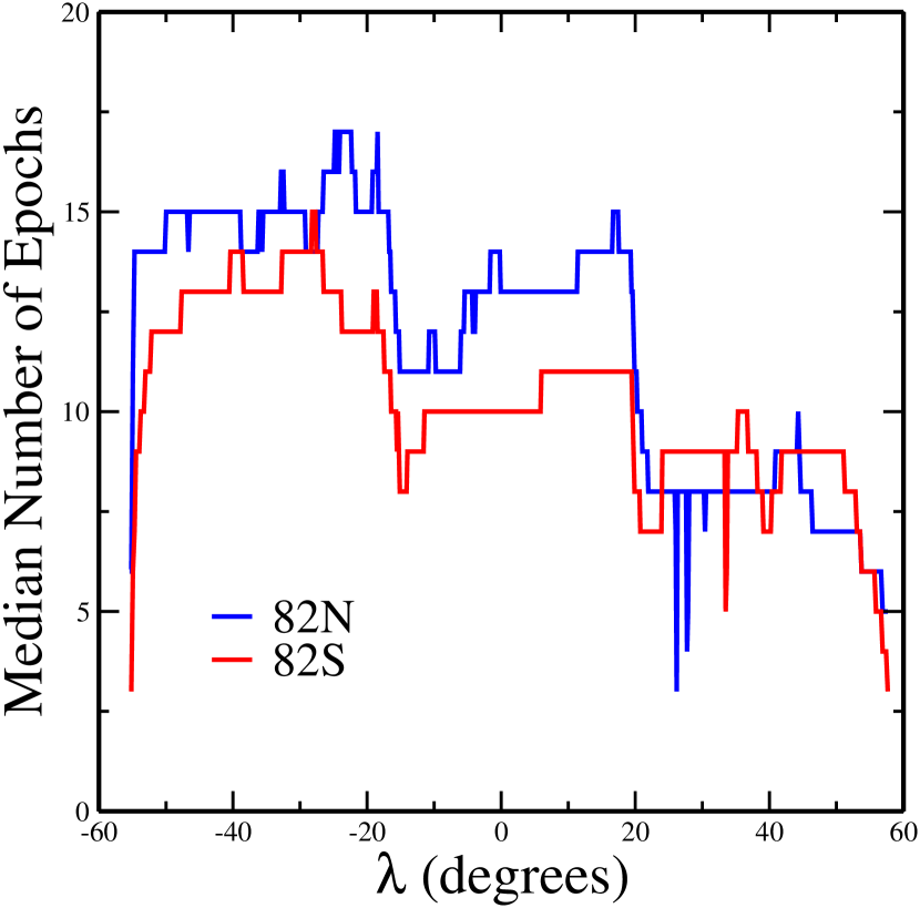
Figure 1: Median number of epochs for each strip as a function of survey coordinate $\lambda$.

As part of normal SDSS operations, the Southern Equatorial stripe has been scanned repeatedly; each idependent scan is assigned a unique run number. This stripe is centered along 0 $DEC$, running from -51 to 59 degrees in $RA$ (J2000). In SDSS survey coodinates, the stripe runs from $-56<\lambda<58$. Figure 1 shows the number of repeat scans (i.e. epochs) for the central scanlines in the two strips contained in the Equatorial stripe. For the purposes of this project, we restrict ourselves to the areas at least 10 epochs deep.

Within this region, we perform a simple position matching amongst the objects identified in each run by the photometric pipeline processing software (photo_v5.4; photo, hereafter) using a tolerance of 0$\farcs$5 for each match. Since we are not concerned about completeness for our sample, we exclude any objects flagged by the pipeline as SATUR, SATUR_CENTER, BRIGHT, EDGE BLENDED and NOPETRO_BIG in any of the five bands. These cuts reduce the total number of objects by roughly 10%.

These flag cuts and are sufficient to eliminate most questionable reductions and the angular matching tolerance is sufficient for isolated objects (Pier et al. 2003). However, objects whose images are blended together represent a special challenge to photo. The pipeline tags these objects with the CHILD flag and they represent roughly 20% of the catalog remaining after the aforementioned flag cuts. Since blended objects are a sizeable fraction of the acceptable objects (particularly for bright galaxies, where they comprise over half the population) and the effects of deblending on the observed scatter are potentially important for the SDSS as well as future surveys, we do not exclude them from our main analysis. Rather, we will include a parallel analysis focusing solely on isolated objects so as to separate the effects of deblending from the remainder of the pipeline.

Finally, all the magnitudes used in each epoch have been dereddened using the reddening map of Schlegel, Finkbeiner & Davis (1998). Galactic extinction does not affect the intrinsic scatter of an object since all epochs are observed through the same line of sight, but it is necessary to correctly make the colors cuts we will discuss later on. This will not be exactly correct for stars since their light does not pass through the entire Galaxy, but we will ignore this distinction for the sake of convenience and uniformity.

2.2 Apertures

For photometric objects, there are four relevant apertures used for calculating magnitudes by the photometric pipeline: PSF magnitudes (psfcounts), model magnitudes (counts_model), composite model magnitudes (cmodel_counts), and Petrosian magnitudes (petrocounts). The details of each of these apertures can be found in Stoughton et al. (2002), Abazajian et al. (2003), Abazajian et al. (2004) and Abazajian et al. (2005). For our purposes, a brief description of each will suffice.

psfcounts generates a magnitude from the flux within the local PSF at the position of the object. Rather than a simple Gaussian, photo decomposes the light profile of bright stars in a given field into 3 Karhunen-Loeve modes. Given a collection of nearby stars, photo then interpolates these modes to reconstruct the PSF at any given point on the field. To measure the psfcounts magnitude, photo fits a Gaussian to the distribution of flux for a given object and then corrects that flux by applying the same Gaussian to the reconstructed PSF. Since it only uses the flux within the PSF, this aperture is obviously inappropriate for extended objects, but it does provide excellent magnitudes for stellar objects.

For counts_model, PSF-convolved exponential and deVaucouleurs profiles are fit to the flux distribution in the $r$ band. The best fitting of these two profiles is used to calculate the magnitude in each of the five bands. Since the same aperture is used in each band, this is the preferred magnitude system for calculating galaxy colors.

cmodel_counts is a variation on counts_model. As before, exponential and deVaucouleurs profiles are fit to the flux distribution in the $rprime$ band, making the counts_exp and counts_dev magnitudes, respectively. With these models in place, a second fit is performed to find the optimal combination of the two models to match the observed flux distribution in each band. The fractional contribution for each aperture in each band is stored in the fracDeV parameter and the flux for the cmodel_counts ($f_{\tt cmodel\_counts}$) is given by

$$f_{\tt cmodel\_counts}={\tt fracDeV}f_{{\tt counts\_dev}}+(1-{\tt fracDeV})f_{{\tt counts\_exp}},$$ (1)

where $0\leq{\tt fracPSF}\leq 1$. Since this prescription attempts to capture the total flux in each band, it is the preferred aperture for relatively faint photometric objects, particularly in the bands other than $r$. However, due to the different aperture sizes, it is not appropriate for colors.

petrocounts is a simple flux aperture whose truncation radius is determined by finding the radius at which

$$R_{P}(r)\equiv\frac{\int^{1.25r}_{0.8r}dr^{\prime}2\pi r^{\prime}I(r^{\prime})/\left[\pi(1.25^{2}-0.8^{2})r^{2}\right]}{\int^{r}_{0}dr^{\prime}2\pi r^{\prime}I(r^{\prime})/\left(\pi r^{2}\right)}=0.2,$$ (2)

where $I(r)$ is the azimuthally averaged surface brightness. The petrocounts magnitude is then defined for an elliptical aperture with semi-major axis twice that of the Petrosian radius. These magnitudes are appropriate for relatively bright galaxies where the projected radius can vary strongly and seeing effects are expected to be minimal. They approximate a total magnitude and are, consequently, used primarily for the SDSS spectroscopic galaxy samples. At moderately faint magnitudes ($r>19$), fluctuations in seeing can lead to very large apertures, extending well beyond most of the flux from the galaxy. This can lead to rather striking variations in the magnitude for a given object as well as much larger photometric uncertainties than is seen when using either counts_model or cmodel_counts.

2.3 Coaddition

While magnitudes allow for easy numerical descriptions, in order to calculate the proper covariance between the bands as well as doing a correct coaddition, we need to convert from asinh magnitudes (Lupton, Gunn & Szalay 1999) into flux. For a given band $i$, the conversion of magnitude ($m_{i}$) into flux ($f_{i}$) is given by

$$f_{i}=2F_{0}L_{i}\sinh\left[-m_{i}/P-\ln L_{i}\right]$$ (3)

where $F_{0}=3630.78$ Jy, $P=1.08574$ and $L=[1.4,0.9,1.2,1.8,7.4]\times 10^{-10}$ for the $u$, $g$, $r$, $i$, and $z$ bands, respectively. Similarly, we can convert magnitude errors ($\Delta m_{i}$) into flux errors ($\Delta f_{i}$) using

$$\Delta f_{i}=2\frac{F_{0}\Delta m_{i}}{P}\sqrt{\sinh^{2}\left(-m_{i}/P-\ln L_{i}\right)+L_{i}^{2}}.$$ (4)

Once in flux units, we can calulate the mean flux ($\bar{f}_{i}$) in each band $i$ for a given object as well as the covariance between each of the bands ($C_{f,ij}$):

$${\rm C}_{f,ij}\equiv\frac{1}{N}\sum^{N}_{n=1}\left(f_{n,i}-\bar{f}_{i}\right)\left(f_{n,j}-\bar{f}_{j}\right),$$ (5)

where $f_{n,i}$ is the $n$th epoch measurement of the flux in band $i$ and $N$ is the total number of epochs. When calculating the covariance matrix, it is important to avoid contamination by random superpositions of unrelated objects. Inadvertantly including a much brighter or fainter object in Equation 5 will affect the mean flux, as well as leading to disproportionately strong off-diagonal elements. Our tight position matching criteria and removal of blended objects is sufficient to exclude the vast majority of these cases. To limit the remainder of contamination, we require that each epoch be within 1 luptitude of the mean.

In addition to the covariance matrix, we also will need the regression matrix ($R_{ij}$):

$${\rm R}_{ij}\equiv\frac{{\rm C}_{f,ij}}{\sqrt{{\rm C}_{f,ii}{\rm C}_{f,jj}}}$$ (6)

where we normalize by the variance in each passband. The regression matrix allows us to calculate a number of important quanities. Most importantly, we can convert the diagonal elements of the flux covariance matrix into magnitude errors ($\delta m_{i}$) using the inverse of the transform from Equation 4 and use the regression matrix to generate the magnitude covariance matrix:

$${\rm C}_{m,ij}={\rm R}_{ij}\delta m_{i}\delta m_{j}.$$ (7)

Using ${\rm C}_{m,ij}$, we can calculate proper color errors:

$$\delta(m_{i}-m_{j})^{2} \equiv \left(\delta m_{i}\right)^{2}+\left(\delta m_{j}\right)^{2}-2{\rm C}_{m,ij}$$

$$\delta(m_{i}-m_{j})^{2} = \left(\delta m_{i}\right)^{2}+\left(\delta m_{j}\right)^{2}-2{\rm R}_{ij}\delta m_{i}\delta m_{j}$$ (8)

In order to ensure that the variation we observe between each epoch is unaffected by any possible calibration differences, we must tie the magnitude zero-points in each run together. This requires us to choose one run, the zero run, from each strip which extends the full length of the stripe to use as the basis for the zero-points on that strip (runs 3384 and 4203 for the north and south strips, respectively). This eliminates the use of these runs for determining ${\rm C}_{f,ij}$ but prevents the calculation from being dominated by constant off-sets ranging across all five bands.

To tie the photometric zero-points together, we first divide each scanline into 20 segments. Within each segment, we find all of the stars with psfcounts errors less than 0.05; this typically restricts us to objects brighter than 17th magnitude in a given band (although considerably deeper in $g$, $r$ and $i$). The stars for a given run are matched by position against the zero run in the same strip. We then calculate the mean difference in psfcounts for all of the run’s stars relative to those in the zero run in each band. These mean differences are used as the zero-point offset at the mid-point of that segment. For individual objects within a run, we interpolate based on those mid-points and subtract the resulting zero-point from all of the objects in the run. Typical values for the zero-point offset range from -0.02 to 0.02 magnitudes.

2.4 Selection Cuts

For the purposes of dividing our data set, we convert $\bar{f}_{i}$ into a coadded magnitude ($\bar{m}_{i}$) for each unique object. The most basic cut is a simple magnitude selection, dividing the sample into unit magnitude slices from 17 to 21 in $r$. Within each magnitude slice, we also separate the sources into red and blue objects. A number of possible cuts have been used in previous papers for this purpose. In this analysis, we use the cut determined by Baldry et al. (2004):

$$\bar{u}-\bar{r} < 1.8~{}~{}:~{}~{}{\rm red}$$ (9)

$$\bar{u}-\bar{r} > 1.8~{}~{}:~{}~{}{\rm blue}$$

Finally, we divide objects into stars and galaxies. In the coadded magnitudes, there is a very clean separation of galaxy and stellar loci using the concentration parameter, $c=\bar{m}_{\tt psfcounts}-\bar{m}_{\tt cmodel\_counts}$. A simple cut at

$$c < 0.05~{}~{}:~{}~{}{\rm star}$$ (10)

$$c > 0.1~{}~{}:~{}~{}{\rm galaxy}$$

in $r$ will divide the sample without significant contamination in either group beyond our faint limit at $r=21$. Combining all of these cuts, we have 24 total sub-samples to consider in each band and each aperture. See Table 1 for a listing of the number of unique objects in each sub-sample for each aperture.

2.5 Comparison to Pipeline Errors

Properly computed photometric errors should reflect the variation in subsequent measurements of the same object. To compare the epoch-to-epoch scatter to the magnitude errors coming out of the photometric pipeline, we calculate the following quantity:

$$\chi^{2}_{F,i}=\sum^{N}_{n=1}\left(\frac{f_{n,i}-\bar{f}_{i}}{\Delta f_{n,i}}\right)^{2},$$ (11)

where we have used the nomenclature from Equation 5 and $\Delta f_{n,i}$ is the photometric pipeline flux error on the $n$th epoch observation in band $i$. For correctly calculated errors, $\chi^{2}_{F}$ should be a $\chi^{2}$ distribution peaked around the number of degrees of freedom ($N$). An equivalent quantity for the magnitudes, ($\chi^{2}_{M}$), can be calculated using the epochal magnitudes and errors as well. To the extent that the transformations in Equations 3 and 4 are valid, $\chi^{2}_{F}$ and $\chi^{2}_{M}$ should be equivalent.

To characterize how well the pipeline errors describe the true uncertainties for all of objects within a given selection bin, we sum the values of $\chi^{2}_{M,i}$ for all of the $N^{\prime}$ objects within that bin and compare it to the sum of the degrees of freedom:

$$\chi^{2}_{T,i}=\Sigma^{N^{\prime}}_{n=1}\left(\chi^{2}_{M,i}\right)_{n}~{}~{};~{}~{}N_{T}=\Sigma^{N^{\prime}}_{n=1}\left(N\right)_{n},$$ (12)

where $(\chi^{2}_{M,i})_{n}$ is the magnitude form of Equation 11 for object $n$. Since $\chi^{2}_{T,i}$ is also a $\chi^{2}$ distribution, we expect that

$$\chi^{2}_{N,i}\equiv\chi^{2}_{T,i}/N_{T}$$ (13)

should be near unity for well-characterized photometric pipeline errors. Further, the mean ratio between the pipeline errors and the actual observed scatter should be given by ${\cal R}_{i}\equiv\sqrt{\chi^{2}_{N,i}}$ in each bin.

2.6 Variable Objects

While the methology described above is appropriate for objects where the scatter in successive measurements is due to statistical fluctuations, intrinsic variability can affect our results in two ways. First, this will bias our comparison of the observed scatter to the errors, increasing the disagreement between the two. Second, since the variability in these objects typically happens over a broad spectral range, this will create strong correlations between filters which would otherwise be independent (or at least more weakly correlated). Including even a relatively small fraction of strongly variable objects in a given magnitude/color/object type bin with otherwise uncorrelated filters (as we would expect for stellar objects, for example) can result in moderately strong off-diagonal regression matrix elements for the ensemble average.

To remove these objects, we matched our 10+ epoch objects against the catalog of photometric quasars described in Richards et al. (2004). Quasars show strong photometric variability (Vanden Berk et al. 2004) and the corresponding regression matrices for these objects have very large off-diagonal elements (see §3.2). This makes the median regression matrix determinant for these objects very small ($\sim 0.003$), compared to that of counts_model galaxies ($\sim 0.01$) and the total stellar population ($\sim 0.2$). By selecting objects with regression matrix determinant less than 0.008, we can effectively split our stellar population into variable ($\sim$ 5-10% of the total) and non-variable sub-populations. A similar cut for galaxies using counts_model selects roughly half the sample and the “non-variable” galaxies still show significant off-diagonal elements. Based on this and the fact that we expect little intrinsic variation in galaxy spectral distribution on the time scale of our repeat observations (relatively speaking), we will only consider variability for stellar objects.

3 Results

3.1 Pipeline Errors vs. Observed Scatter

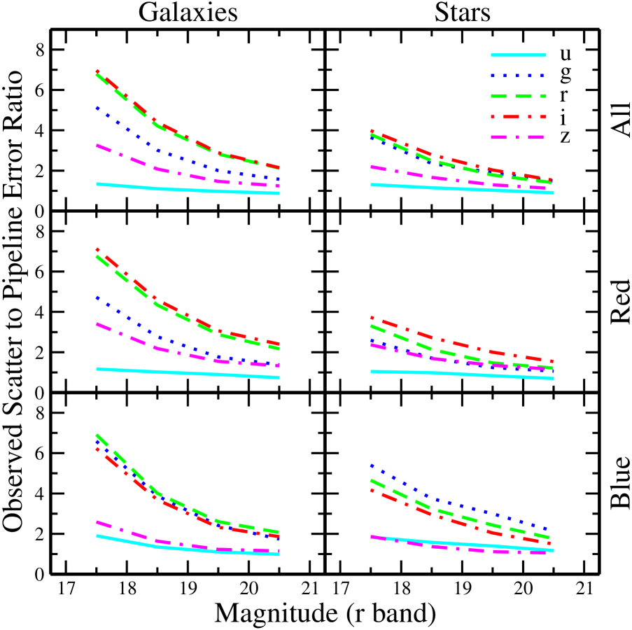
Figure 2: Ratio of observed magnitude errors to photo pipeline errors ($\chi_{\rm N}$) as a function of object type, magnitude and color using counts_model. The $u$ ratio is indicated by the solid lines, $g$ by the dotted line, $r$ by the dashed line, $i$ by the dot-dashed line, and $z$ by the dash-dotted line.

Tables 2 through 5 show the values of $\chi^{2}_{\rm N}$ for the various selection criteria and Figures 2 through 4 show ${\cal R}$, the ratio between the observed scatter and the photo pipeline errors, for each band. In general, we find that bright objects typically display much larger scatter than one would expect based on the photo errors; the values of $\chi^{2}_{\rm N}$ in Tables 2 through 5 are consistent with the peaks in the various distributions of $\chi^{2}_{F}$, confirming our contention in §2.5 that the aggregate would be $\chi^{2}$ distribution. The excess scatter was most prominent with counts_model and least with psfcounts, but exists for all apertures. It should be noted, however, that despite the seemingly large ratios between the observed scatter and the pipeline errors, the observed scatter at the bright end remains very small in an absolute sense (this can be easily inferred from the values of the color errors given in Tables 6 through  11 described in §3.3). As objects become fainter, the agreement between photo errors and the observed scatter generally improved. The $u$ band scatter also tended to be much better matched by the pipeline errors at all magnitudes in all apertures (see Baldry et al. 2005 for more details on $u$ band errors). This behavior is consistent with the notion that the bright end scatter can be strongly influenced by the details of modelling the light distribution, while at the faint end photon noise becomes the dominant source of scatter. Finally, in all apertures, stars showed a much stronger color dependence on $\chi^{2}_{\rm N}$ than galaxies, with blue stars usually giving a much larger observed scatter relative to their photo errors than red stars (see §3.4 for more details).

For counts_model, the values of $\chi^{2}_{\rm N}$ tended to be most extreme in the $r$ and $i$ bands. In general, the photo errors were under-estimated by at least a factor of 2 for almost all combinations of magnitude, object type and color, and by as much as a factor of 6 in some cases. Stars, however, typically had smaller values of $\chi^{2}_{\rm N}$ for a given magnitude and color. Like counts_model, the photo errors for cmodel_counts were, in general, strongly under-estimated relative to the observed scatter, albeit to a lesser degree than counts_model. cmodel_counts also showed the same $\chi^{2}_{\rm N}$ split between stars and galaxies. petrocounts and psfcounts errors typically showed much better agreement between the photo errors and the observed scatter than either of counts_model or cmodel_counts.

3.2 Regression Matrices

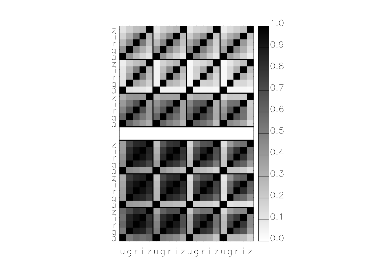
Figure 5: Regression matrices for objects using counts_model, galaxies in the lower block and stars in the upper block. The $5\times 5$ matrices separate the total sample of unique objects into 4 magnitude bins ($17<r<18$, $18<r<19$, $19<r<20$, $20<r<21$) and 3 color bins: no color cut, red objects ($u-r>1.8$) and blue objects ($u-r<1.8$). In each block, the top row gives the regression matrices for objects with no color cut, the middle row for the red objects and the bottom row for the blue objects. Going from left to right runs from the brightest to faintest magnitude cut in each row.

Figures 5 through 7 show the mean regression matrices for objects that fall within each selection bin for each aperture. We do not plot the regression matrices for galaxies using the psfcounts magnitudes nor for stars with the petrocounts magnitudes, as these systems are intrinsically inappropriate for those objects.

The primary determining factor for the strength of the off-diagonal elements of the regression matrix was object type. Stars observed using counts_model, cmodel_counts, and psfcounts produced $R$ matrices that were nearly identical, with strong off-diagonal elements for blue stars ($R_{u,g},R_{g,r},R_{r,i}\sim 0.4-0.6$) and weaker equivalent elements (0.2-0.4) for red stars. The amplitude of the off-diagonal elements was somewhat smaller for the psfcounts and cmodel_counts regression matrices compared to the counts_model regression matrices, but the relative strength of the elements within each associated matrix was very similar. Likewise, all three apertures showed the same slight evolution toward weaker off-diagonal elements for fainter samples relative to bright ones.

For extended objects, the strongest off-diagonal elements were found using the counts_model magnitudes. This is not surprising given that the aperture used in this method is not independently fit in each band. With the exception of $R_{u,g}$, the nearest off-diagonal elements using counts_model typically ranged from 0.6 to 0.9, with similarly strong elements in the $R_{g,i}$ elements. By comparison, the same terms in the regression matrices from cmodel_counts and petrocounts were almost always less than 0.5, usually much less. As with stars, the off-diagonal amplitude for all apertures decreases as a function of increasing magnitude. For cmodel_counts and petrocounts, the evolution is quite strong relative to that seen in counts_model; at the faintest magnitudes the regression matrices for cmodel_counts and petrocounts are nearly diagonal, while the off-diagonal elements for counts_model have diminished by only 10-15%.

Separating galaxies by color, we find that the regression matrices for blue galaxies typically have stronger terms along the $u$ column than those for red galaxies; clearly these terms are suppressed in the latter matrices by the relatively faint $u$ magnitudes for those sources. The $R_{g,r}$, $R_{r,i}$ and $R_{g,i}$ terms are generally very similar regardless of aperture, while red galaxies have stronger $R_{i,z}$ terms. These tendencies are consistent regardless of magnitude or aperture.

3.3 Color Errors

To estimate the relative importance of covariance on color errors and to compare with the photo errors and the observed scatter, we calculate four quantities for the most commonly used colors ($u-g$, $g-r$, $r-i$, and $i-z$):

$\bullet$ Observed Errors: The measured error based on the mulit-epoch data measured independently for each color for objects in a given magnitude/object type/color bin.
$\bullet$ Proper Errors: Using the observed scatter in each band ($\delta m_{i}$) and the appropriate regression matrix, we calculate the color error as given in Equation 2.3. If the errors are Gaussian, then the proper errors should match the observed errors closely.
$\bullet$ Naive Errors: Like proper errors, except that the covariance term is omitted. The ratio between the proper and naive errors indicates the strength of the covariance between bands.
$\bullet$ photo Errors: Using $\chi_{N}$, we transform the observed scatter in each band into an estimate of the mean photo errors for the objects in each bin. Since we do not have a proper covariance matrix for the photo errors, we calculate the color errors without it.

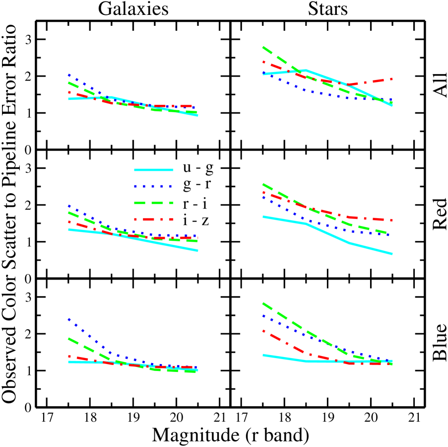
Figure 8: Ratio of observed color errors to photo pipeline color errors as a function of object type, magnitude and color using counts_model. $u-g$ error ratio is indicated by the solid lines, $g-r$ by the dotted line, $r-i$ by the dashed line, and $i-z$ by the dot-dashed line.

Tables 6 through  11 provide these quantities as a function of aperture, object type, magnitude, and color. Figures 8 through 10 show the ratio between the observed color errors and the photo color errors. It is worth noting at the outset that colors measured with apertures other than counts_model and psfcounts (and only for stars in the latter case) are not meant to be meaningful, so disagreements between the observed scatter and the photo color errors are not likely to be relevant to any current or future research. For completeness, however, we will touch on them briefly.

As expected by the strong off-diagonal elements in the galaxy counts_model regression matrices, the naive errors here were typically larger than the proper errors by 20-60%. With the exception of the $u-g$ color, the proper errors generally matched the observed color scatter very well. Indeed, the match between proper errors and the observed scatter for the other three colors was very good regardless of aperture, object type, magnitude or color. This verifies that, fundamentally, the scatter in the colors is well modeled by a Gaussian. $u-g$ errors were typically under-estimated by the proper errors, although part of this discrepancy may have been due to $u$ drop-outs. Despite the strong covariance between bands seen in the regression matrices, photo errors matched the observed scatter nearly as well as the proper errors (Figure 8), although less so at bright magnitudes where they tend to under-estimate the color errors.

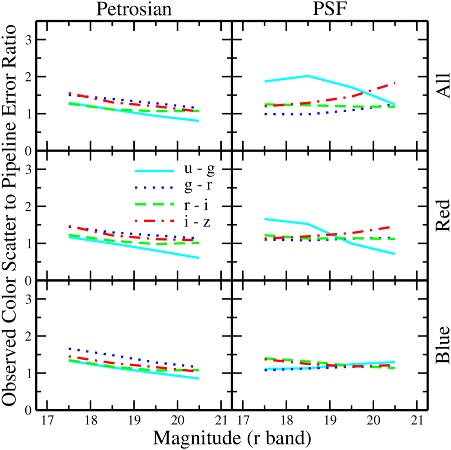
Figure 10: Same as Figure 8, but for galaxies using petrocounts and stars using psfcounts.

For psfcounts , the agreement between the proper error, the photo error and the observed scatter was also quite good. The photo errors were typically smallest of the three, but usually by no more than 10%. photo errors were particularly good for blue stellar objects (Figure 10).

While the difference between photo errors and the observed scatter in each band generally cancelled the lack of a covariance term for counts_model galaxies and psfcounts stars, the photo color errors for stars observed with counts_model were under-estimated by as much as 100% (Figure 8). This was true regardless of magnitude or object color, although fainter stars tended to have smaller differences between the photo color errors and the observed scatter.

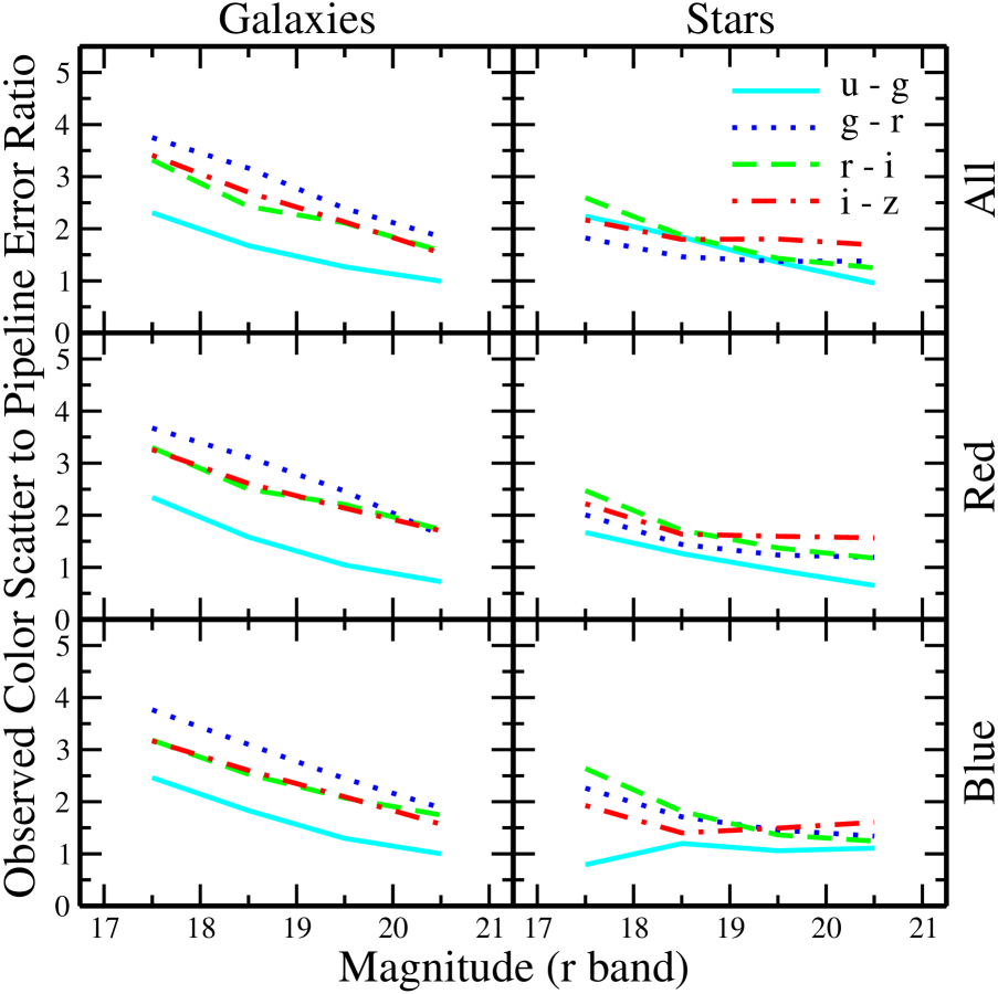
Figure 9: Same as Figure 8, but using cmodel_counts.

Likewise, the color errors from photo were under-estimated for all observed with cmodel_counts magnitudes by factors as large as 2-3. In all cases, the color errors were under-estimated by at least 25% (Figure 9). photo color errors were generally under-estimated by 10-20% for petrocounts (Figure 10).

3.4 Variability Results

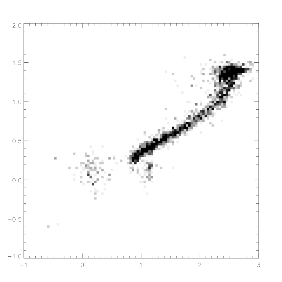
Figure 11: Coadded $u-g$ vs. $g-r$ for variable stellar objects.

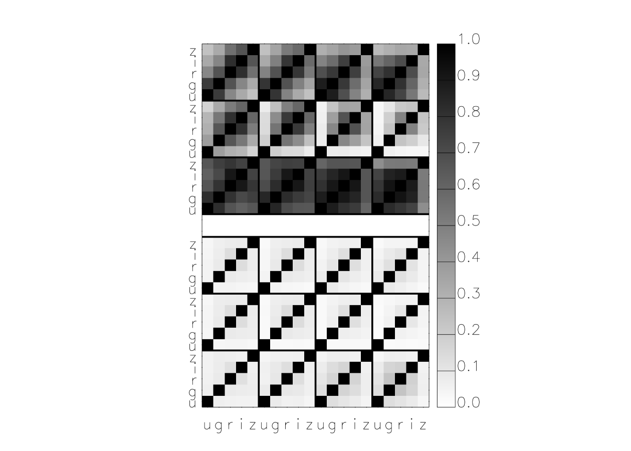
Figure 12: Same as Figure 5, but for variable stars objects using psfcounts in the upper block and non-variable stars in the lower block.

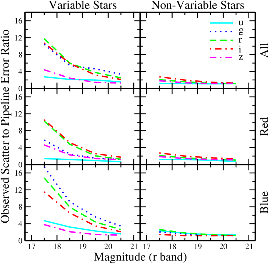
Figure 15: Same as Figure 2, but for variable and non-variable stars using counts_model.

As mentioned in §2.6, selecting highly variable objects by cutting on regression matrix determinant yields 5-10% of the total stellar population in any given magnitude/color/aperture bin. As shown in Figure 11, the objects selected by the variability cut are primarily located in four regions: the low redshift quasar locus, F stars at the blue end of the stellar locus, the K & M stars at the red end of the stellar locus and the blue horizontal branch spur extending below the blue end of the stellar locus. This is consistent with where we would expect to find highly variable objects in color-color space, as well as the results found by Ivezić et al. (2000). Figures 12 through 14 give the variable and non-variable regression matrices as a function of magnitude and color for the counts_model, cmodel_counts and psfcounts apertures and Figures 15 through 17 do the same for the associated ${\cal R}$ measurements (the values for $\chi^{2}_{\rm N}$ are in Tables 12 through 14).

As expected by the variability cut, the variable objects show very strong covariance between filters. Contrarily, the non-variable object have nearly independent magnitude errors. The behavior of all three apertures is nearly indentical as a function of color and magnitude, as seen in the full stellar sample. This confirms our earlier contention in §2.6 that the covariance between filters for stellar objects seen in Figures 5 through 7 was driven almost entirely by a small population of highly variable objects in the sample, as opposed to the model induced covariance seen in counts_model for galaxies. Further, we can see from the variation of the regression matrices with color that objects at the blue end of the stellar locus are more highly variable over the entire optical spectrum than those at the red end of the stellar locus.

Although we did not explicitly select objects with large values of $\chi^{2}_{\rm N}$ with our variability cut, clearly the variable and non-variable objects have a wide disagreement in $\chi^{2}_{\rm N}$ for all magnitude and colors. For the latter sub-population, the pipeline errors estimate the observed scatter much better than for the entire population (as seen in Tables 2, 3, and 5), while variable objects display a much larger scatter than the pipeline errors would suggest. Further, while the distribution of $\chi^{2}_{F}$ values for the non-variable objects is well matched to the expected $\chi^{2}$ distribution, the values of $\chi^{2}_{\rm N}$ for the variable objects are dominated by a sizeable fraction of extreme outliers ($\chi^{2}_{F}/N>20$). This is an excellent confirmation that our variability criteria, while perhaps not capturing all of the variable objects, does select a sub-population with much larger scatter than photon noise would predict. Futher, as was seen with the regression matrices, most of the disagreement with the pipeline errors appears to be driven by a relatively small population of highly variable objects. Likewise, the values of $\chi^{2}_{\rm N}$ for blue objects are typically much larger than those for red objects, behavior that is consistent regardless of aperture. This contrasts strongly with the non-variable objects, where the color variation is almost nil (as one would expect for relatively weak variation of the PSF with color over this range). Finally, we can see that blue stellar objects show a stronger disagreement relative to red objects at fainter magnitudes than at brighter magnitudes. However, this may be an artifact of our selection criteria, which would tend to lose red variable objects at brighter magnitudes due to their much lower flux in $u$.

3.5 Isolated vs. Deblended Objects

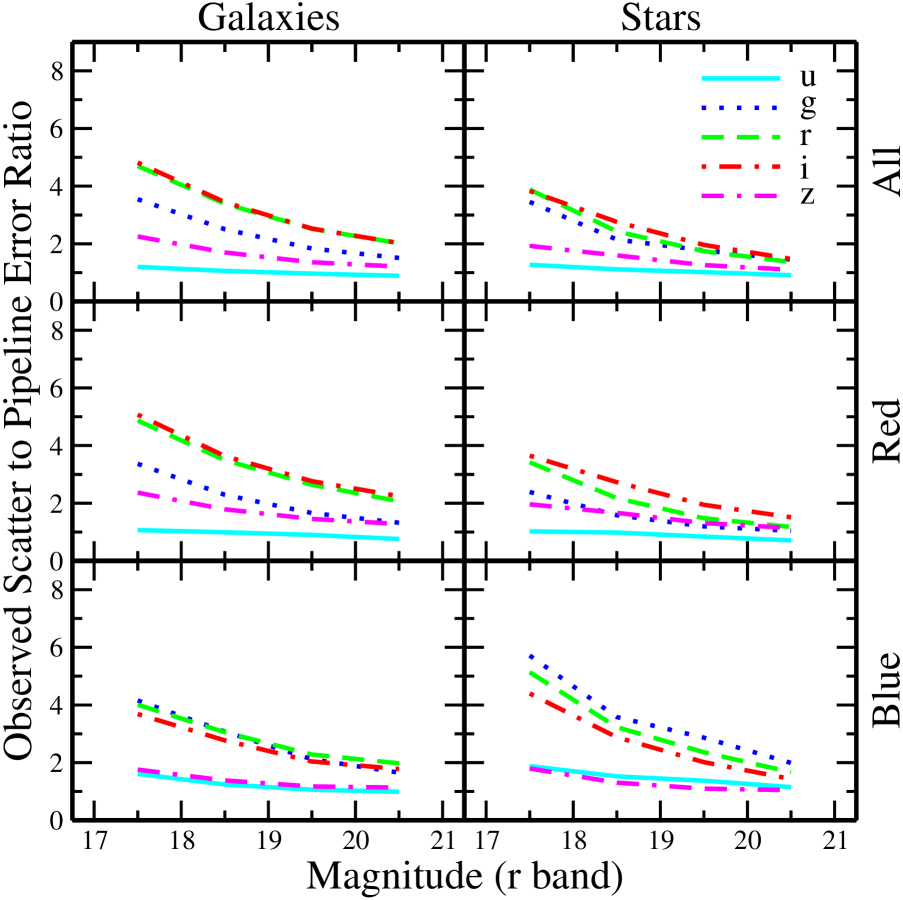
Figure 18: Same as Figure 2, but for isolated objects. The scaling on the y-axis is the same as in Figure 2 to demonstrate the difference in the scatter for blended versus isolated objects.

Figures 18 through 20 show ${\cal R}$ for the isolated objects. In all three cases, we keep the scaling on the y-axis identical to those where we have included the deblended objects (Figures 2 through 4). As one might expect, the effect of deblending on magnitude scatter shows up strongest for relatively bright galaxies, while faint galaxies and stars at all magnitudes are relatively unaffected by whether the object is isolated or part of a blend. One can see from Table 1 that the fraction of deblended objects in a given magnitude/object type bin follows a similar pattern: a large fraction of bright galaxies have been deblended, but this ratio shrinks considerably as galaxies grow fainter; the stellar ratio stays roughly constant with magnitude. The contrast between isolated and blended objects is strongest for petrocounts, where R is nearly unity for isolated objects at all magnitudes, while R for the full data set is above 2 at the bright end. cmodel_counts shows similar but less dramatic behavior, while counts_model is only changed by 20-30% at the bright end for isolated versus blended objects.

Unlike R, the regression matrices for the isolated objects were nearly identical to the full data set, with individual values of $R_{i,j}$ varying by less than 5%.

4 Error Translation & Covariance

With the results of the previous sections, we can develop a prescription for translating photo errors into observed scatter as well as generating a covariance matrix. Since we are primarily interested in applying this method to correct color errors, we will concentrate on galaxies using counts_model and petrocounts and stars using psfcounts.

The basic relation between the observed scatter $\delta m$ and the pipeline error $\Delta m$ is

$$\delta m\equiv{\cal R}\Delta m,$$ (14)

where the curves for R as a function of aperture, object type, magnitude and color are given in Figures 2 through 4. To model R, we will typically need two pieces: a term that varies with magnitude to characterize the transition between errors dominated by modeling fits to those dominated by photon noise and a constant term representing the floor on the scatter (or equivalently the gain on the CCDs). We can approximate these requirements with a simple power law plus a constant:

$${\cal R}(m)=\left(\frac{m}{m_{0}}\right)^{\alpha}+\beta,$$ (15)

where $\alpha$, $m_{0}$ and $\beta$ are a function of filter, aperture and object type. For the most accurate results, these parameters should also be a function of color, but using the fits ignoring color is sufficient for most cases. Table 15 presents the fits for the three cases mentioned above as well as galaxies using cmodel_counts. Equation 15 does an excellent job of modeling ${\cal R}$ for counts_model and cmodel_counts galaxies (with the exception of the $u$ band in the latter case). It is a reasonably good approximation of the variation for petrocounts galaxies, with the same $u$ caveat. For psfcounts, the variation of ${\cal R}$ with magnitude is small enough that we can approximate it best using just the $\beta$ parameter, setting $\alpha$ to zero. To the extent that we are able to cleanly make the measurements, extrapolating Equation 15 brightward and faintward of $17\leq r\leq 21$ matches the observed values of ${\cal R}$.

To calculate the covariance matrix, we focus on reproducing the regression matrix as a function of magnitude and color for a given aperture/object type combination. Once the regression matrix is calculated, we can conver it to a covariance matrix according to Equation 7.

To handle the variation in the regression matrix as a function of color, we use two matrices: the red object regression matrix ($R_{R}$) and the color differential matrix ($R_{\rm D}\equiv R_{\rm B}-R_{\rm R}$, where $R_{\rm B}$ is the blue object regression matrix). To produce the regression matrix, we combine $R_{\rm R}$ and $R_{\rm D}$ using a sigmoid function:

$$R=R_{\rm R}+\left(1-\left[1+{\rm exp}\left(-\frac{{\cal C}-{\cal C}_{R}}{\sigma_{R}}\right)\right]^{-1}\right)R_{\rm D},$$ (16)

where ${\cal C}$ is the color used to separate red and blue objects, ${\cal C}_{R}$ is the dividing line between red and blue and $\sigma_{R}$ controls the width of the transition. For our implementation, ${\cal C}\equiv u-r$ and ${\cal C}_{R}=1.8$ as set in Equation 2.4. For counts_model galaxies we set $\sigma_{R}\equiv 0.15$. The values for $R_{\rm R}$ and $R_{\rm D}$ are given in Table 16.

In addition to setting the amplitude of the off-diagonal elements of $R$ according to object color, we also need to take into account the observed variation of the off-diagonal elements as a function of magnitude as described in §3.2. Because objects have intrinsic colors and the five filters have different depths, we need to model this variation separately for each element of the regression matrix. By calculating the regression matrix for each unique object and dividing each element by the corresponding element from the appropriate regression matrix produced by Equation 16. This ratio can be modeled as a function of $r$ using a simple power law:

$${\cal A}_{ij}(r)=\left(\frac{r}{r_{0,ij}}\right)^{A_{ij}}$$ (17)

The values for $r_{0,ij}$ and $A_{ij}$ are given in Table 17. The addition of this term modifies Equation 16 to

$$R_{ij}={\cal A}_{ij}(r)\left(R_{{\rm R},ij}+\left(1-\left[1+{\rm exp}\left(-\frac{{\cal C}-{\cal C}_{R}}{\sigma_{R}}\right)\right]^{-1}\right)R_{{\rm D},ij}\right),$$ (18)

where the diagonal elements of $R$ are set to unity by definition.

As one might expect from the generally noisy behavior of the $u$ filter, the variation for the regression elements involving that filter tends to be much stronger than other filter combinations. Because of this behavior, the regression matrices produced by Equation 18 are singular for blue galaxies with $r<16$. For these galaxies, using $r=16$ should produce a suffciently accurate regression matrix for most purposes.

5 Conclusions & Discussion

In this paper, we have presented an analysis of the observed photometric covariance for the five SDSS filters drawn from multiple repeat scans of the southern equatorial stripe. Given the large number of objects in the stripe we were able to sub-divide the total sample by magnitude, object type and color. Likewise, we looked at the effect of the standard SDSS apertures (counts_model, cmodel_counts, psfcounts, petrocounts) on the photometric covariance. In general we find that the photometric pipeline (photo) errors under-estimate the observed scatter in the five filters, although the degree of disagreement was a strong function of aperture and magnitude. psfcounts errors were typically under-estimated by 20-50%, while the ratio of counts_model and cmodel_counts observed scatter to photo errors was as large as 6 at bright magnitudes, tailing off to a ratio of 2 at the faint limit.

The degree of covariance between filters was primarily a function of object type. Stellar objects produced similar regression matrices regardless of aperture. The amplitude of the off-diagonal elements in the regression was a weak function of magnitude, typically dropping by 10-20% from the brightest to the weakest samples. This variation was weakest in psfcounts, the preferred aperture for SDSS quasar target selection. When variable stellar objects were removed from the sample, the correlation between filters was negligible and the pipeline errors for psfcounts were an excellent match for the observed scatter.

For galaxies, the regression matrix was a strong function of aperture. Galaxies observed with counts_model (the preferred aperture for galaxy colors) were strongly covariant, showing correlations between the $g$, $r$ and $i$ bands in excess of 70% for all colors and magnitudes. This strong covariance should lead to a large over-estimation of the color errors if neglected. However, since the magnitude errors in counts_model were so strongly under-estimated, the photo color errors were typically under-estimated by 10-20% relative to the observed color scatter, although this did rise to 100% at the bright limit. The scatter at the bright end was also a function of whether or not the galaxy had been deblended from a larger group. Bright isolated galaxies had smaller scatter relative to their deblended counterparts, although the ratio between the observed scatter and pipeline errors remained large.

Given all of this, we can make the following prescription:
$\bullet$ For Stellar Objects: Using psfcounts is recommended for both magnitudes and colors. In both cases, the pipeline errors match the observed scatter very well, provided that the object is not intrinsically variable. For quasars and variable stars (5-10% of the total population of stellar objects), the scatter can be considerably larger than the pipeline errors and will tend to be strongly correlated between filters.
$\bullet$ For Galaxy Magnitudes: The preferred aperture is cmodel_counts, although petrocounts is acceptable for objects bright enough to be in the main SDSS galaxy sample ($r<17.5$). In either case, the pipeline errors can be corrected using Equation 15 with the appropriate parameters from Table 15.
$\bullet$ For Galaxy Colors: The preferred aperture is counts_model. At the faint end, the color errors from the pipeline are only slightly smaller than the observed scatter, but one should be aware that the ratio between the observed scatter and the pipeline errors can be larger than 2 for bright objects. For applications like photometric redshifts, where the entire galaxy SED can be important, one should calculatd the full magnitude covariance matrix using Equations 15 and 18.

Despite the fact that the differences between the observed color errors in the SDSS and the color errors from the processing pipeline were generally small, the existence of covariance between magnitude bands is an intrinsic feature of multi-waveband photometry. This makes it an issue that will need to be addressed by nearly all future surveys. The degree of precision required for color-based target selection and photometric redshifts to meet these surveys’ science goals will place enormous demands on the full photometric system, hardware and software. Given the strength of even the far off-diagonal elements of the counts_model regression matrices, it is clear that incorporating the full covariance matrix into the data model for these surveys will be absolutely necessary to extract the full statistical power from these data sets.

This analysis suggests that future surveys will need to incorporate large numbers of repeated scans into the early stages of their survey operations. This data set will provide an invaluable tool for empirically checking the ability of the photometric system to recover the observed covariance for objects as well as excellent means for testing the efficiency and completeness of target selection, photometric redshifts and other color-based selection algorithms. Likewise, it would also serve as an excellent test bed for future refinements of the photometric pipeline software.

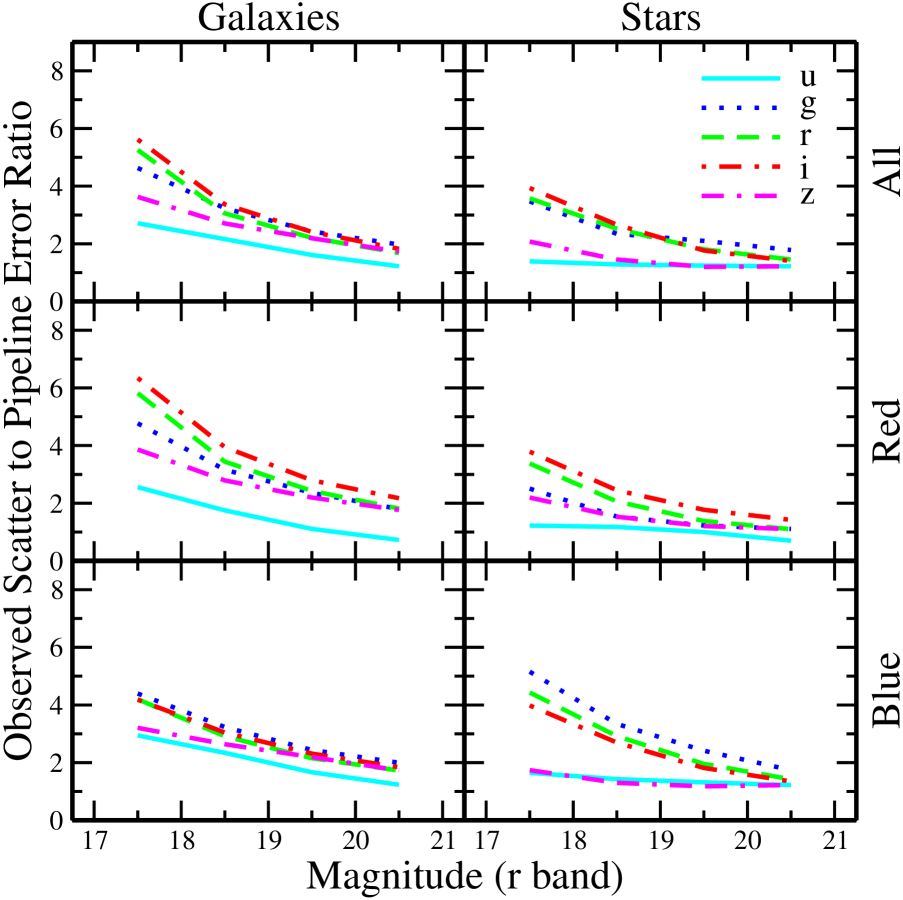
Figure 3: Same as Figure 2, but using cmodel_counts.

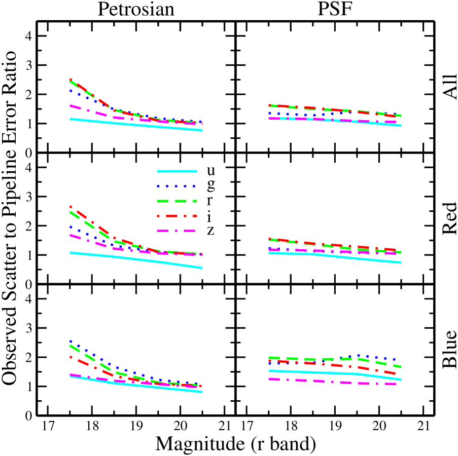
Figure 4: Same as Figure 2, but for galaxies using petrocounts and stars using psfcounts.

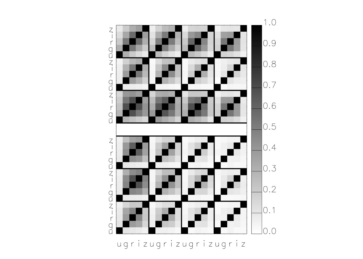
Figure 6: Same as Figure 5, but for cmodel_counts.

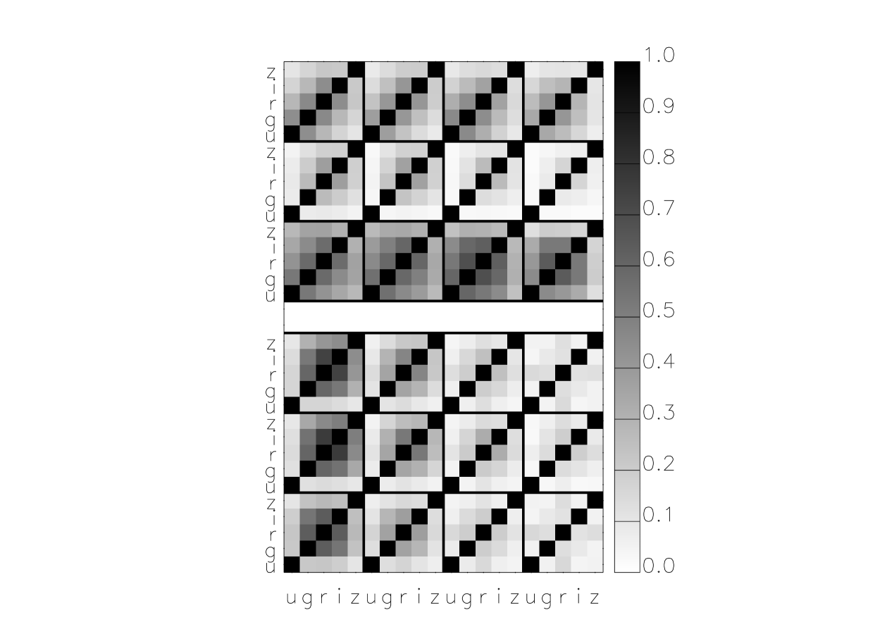
Figure 7: Same as Figure 5, but for psfcounts in the upper block and petrocounts in the lower block.

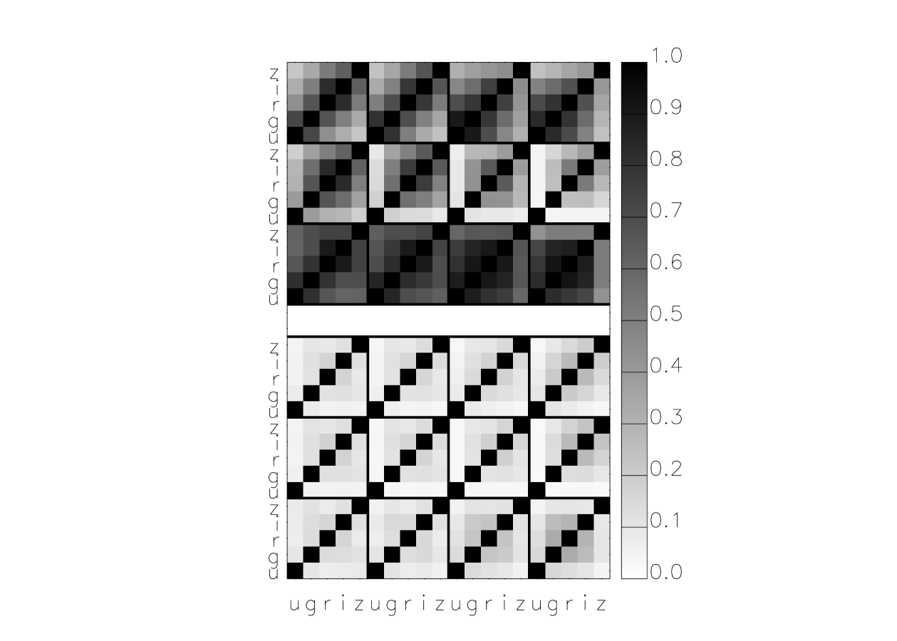
Figure 13: Same as Figure 12, but using counts_model but for variable stars.

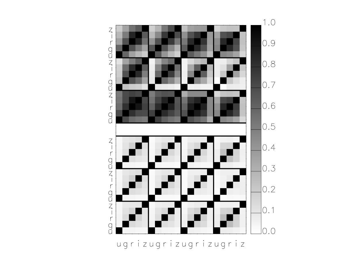
Figure 14: Same as Figure 12, but using cmodel_counts but for variable stars.

Figure 16: Same as Figure 2, but for variable and non-variable stars using cmodel_counts.

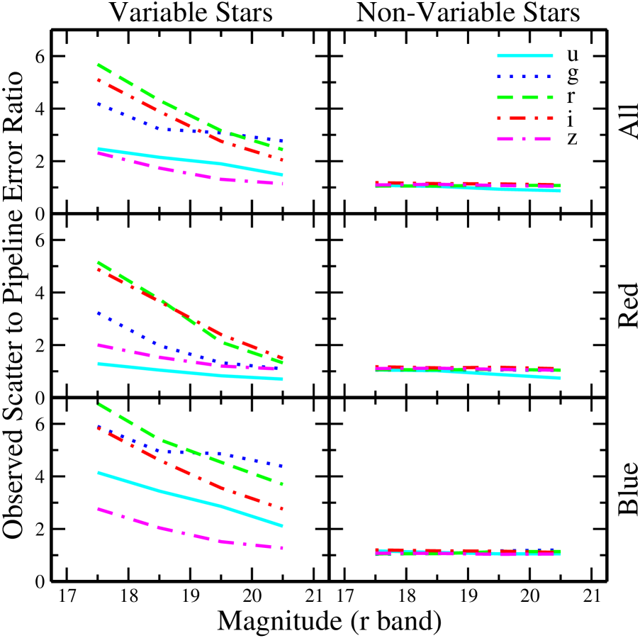
Figure 17: Same as Figure 2, but for variable and non-variable stars using psfcounts.

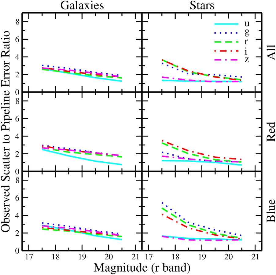
Figure 19: Same as Figure 18, but using cmodel_counts.

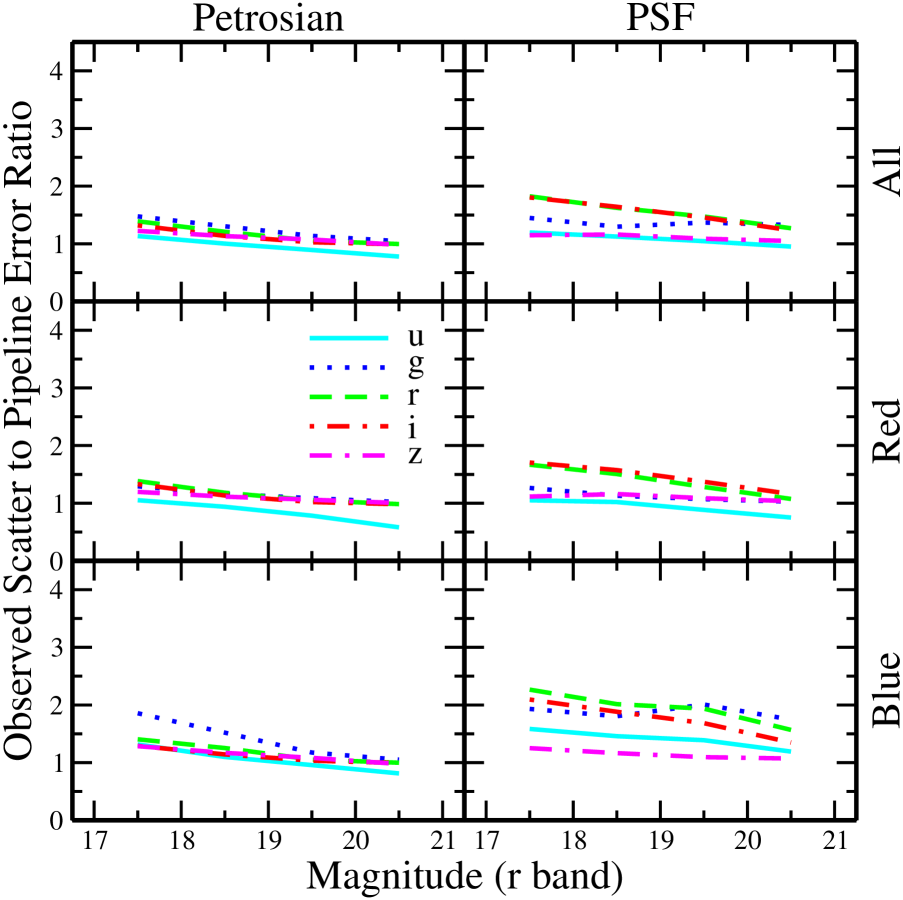
Figure 20: Same as Figure 18, but for galaxies using petrocounts and stars using psfcounts.

Table 1: Unique objects per magnitude and color bin for objects with at least 10 epochs.

		Galaxies				Stars
Aperture	Mag. Limit	All	Red	Blue		All	Red	Blue
All counts_model	$17<r<18$	14505	11744	2761		52293	40258	12035
	$18<r<19$	48411	37301	11110		68046	53566	14480
	$19<r<20$	141876	98927	42949		99440	75698	23742
	$20<r<21$	335314	196027	140287		140187	98770	41417
Isolated counts_model	$17<r<18$	7535	5972	1563		37266	28791	8475
	$18<r<19$	32204	24385	7819		53144	42539	10605
	$19<r<20$	106569	72003	34566		78840	60630	18210
	$20<r<21$	283497	157933	125564		117163	81642	35521
All cmodel_counts	$17<r<18$	14631	8943	5688		52294	39629	12665
	$18<r<19$	48993	17294	31699		68046	48462	19584
	$19<r<20$	143509	17339	126170		99442	39389	60053
	$20<r<21$	338506	10423	328083		140176	16687	123489
Isolated cmodel_counts	$17<r<18$	7629	4364	3265		37268	28307	8961
	$18<r<19$	32714	10532	22182		53143	38364	14779
	$19<r<20$	108011	10962	97049		78843	30968	47875
	$20<r<21$	285944	6991	278953		117157	13032	104125
All petrocounts	$17<r<18$	13588	10210	3378		$\cdots$	$\cdots$	$\cdots$
	$18<r<19$	46108	31527	14581		$\cdots$	$\cdots$	$\cdots$
	$19<r<20$	136891	77778	59113		$\cdots$	$\cdots$	$\cdots$
	$20<r<21$	312519	126860	185659		$\cdots$	$\cdots$	$\cdots$
Isolated petrocounts	$17<r<18$	6884	4941	1943		$\cdots$	$\cdots$	$\cdots$
	$18<r<19$	30400	20114	10286		$\cdots$	$\cdots$	$\cdots$
	$19<r<20$	101991	55025	46966		$\cdots$	$\cdots$	$\cdots$
	$20<r<21$	260567	99102	161465		$\cdots$	$\cdots$	$\cdots$
All psfcounts	$17<r<18$	$\cdots$	$\cdots$	$\cdots$		52233	40070	12163
	$18<r<19$	$\cdots$	$\cdots$	$\cdots$		67857	53280	14577
	$19<r<20$	$\cdots$	$\cdots$	$\cdots$		98537	74636	23901
	$20<r<21$	$\cdots$	$\cdots$	$\cdots$		137671	96214	41457
Isolated psfcounts	$17<r<18$	$\cdots$	$\cdots$	$\cdots$		37207	28645	8562
	$18<r<19$	$\cdots$	$\cdots$	$\cdots$		53001	42312	10689
	$19<r<20$	$\cdots$	$\cdots$	$\cdots$		78123	59804	18319
	$20<r<21$	$\cdots$	$\cdots$	$\cdots$		114798	79362	35436

Table 2: $\chi^{2}_{\rm N}$ values for each band as a function of object type, magnitude and color for counts_model.

Object Type	Magnitude Limit	Color Cut	$u$	$g$	$r$	$i$	$z$
Galaxy	$17<r<18$	All	1.80	26.4	46.1	48.5	10.7
		Red	1.37	22.3	45.8	50.8	11.6
		Blue	3.63	43.4	47.8	38.8	6.69
	$18<r<19$	All	1.22	9.07	17.8	19.3	4.33
		Red	1.04	7.66	18.8	21.1	4.76
		Blue	1.81	15.1	16.1	13.6	2.67
	$19<r<20$	All	0.95	4.01	7.97	8.33	2.16
		Red	0.80	3.12	8.29	9.39	2.39
		Blue	1.22	5.83	6.78	5.41	1.52
	$20<r<21$	All	0.77	2.48	4.51	4.61	1.55
		Red	0.54	1.90	4.70	5.76	1.76
		Blue	0.97	3.02	4.27	3.46	1.32
Star	$17<r<18$	All	1.72	13.3	14.4	15.9	4.82
		Red	1.09	6.74	10.9	13.9	5.62
		Blue	3.35	29.2	21.7	17.4	3.49
	$18<r<19$	All	1.33	5.55	6.20	7.78	2.77
		Red	0.97	2.92	4.56	7.41	2.86
		Blue	2.49	14.1	10.4	8.69	1.87
	$19<r<20$	All	1.06	3.60	3.18	4.13	1.68
		Red	0.70	1.54	2.17	4.01	1.83
		Blue	1.95	8.97	5.92	4.18	1.24
	$20<r<21$	All	0.82	2.21	1.96	2.32	1.24
		Red	0.49	1.13	1.47	2.36	1.32
		Blue	1.37	4.57	3.10	2.22	1.10

Table 3: Same as Table 2, but for cmodel_counts.

Object Type	Magnitude Limit	Color Cut	$u$	$g$	$r$	$i$	$z$
Galaxy	$17<r<18$	All	7.36	21.4	27.6	31.6	13.1
		Red	6.53	22.7	33.8	40.2	14.9
		Blue	8.67	19.3	17.6	17.5	10.3
	$18<r<19$	All	4.67	10.4	9.33	11.4	7.31
		Red	3.06	9.99	11.8	15.6	7.79
		Blue	5.47	10.5	8.50	9.26	6.97
	$19<r<20$	All	2.60	5.89	4.86	5.81	4.81
		Red	1.23	5.57	5.89	7.81	4.82
		Blue	2.77	5.94	4.63	5.34	4.81
	$20<r<21$	All	1.49	3.90	2.83	3.34	2.99
		Red	0.53	3.24	3.29	4.72	3.12
		Blue	1.52	3.98	2.97	3.39	3.00
Star	$17<r<18$	All	1.94	12.1	12.8	15.5	4.32
		Red	1.49	6.28	11.4	14.3	4.83
		Blue	2.71	26.6	19.6	15.9	3.02
	$18<r<19$	All	1.65	5.50	6.36	7.09	2.12
		Red	1.38	2.36	4.24	6.00	2.34
		Blue	2.04	11.2	8.53	7.28	1.69
	$19<r<20$	All	1.55	4.42	3.27	3.13	1.44
		Red	1.00	1.51	1.92	3.14	1.45
		Blue	1.73	5.83	3.82	3.29	1.39
	$20<r<21$	All	1.49	3.18	2.12	1.97	1.49
		Red	0.49	1.23	1.21	2.02	1.21
		Blue	1.49	3.02	2.02	1.82	1.50

Table 4: Same as Table 2, but for petrocounts.

Object Type	Magnitude Limit	Color Cut	$u$	$g$	$r$	$i$	$z$
Galaxy	$17<r<18$	All	1.33	4.55	6.03	6.36	2.61
		Red	1.16	3.88	6.13	7.13	2.83
		Blue	1.84	6.55	5.76	4.06	1.96
	$18<r<19$	All	1.02	2.21	2.15	2.10	1.46
		Red	0.88	1.73	2.15	2.53	1.48
		Blue	1.23	2.80	2.21	1.83	1.42
	$19<r<20$	All	0.79	1.39	1.26	1.21	1.15
		Red	0.58	1.22	1.27	1.21	1.12
		Blue	0.92	1.50	1.27	1.18	1.16
	$20<r<21$	All	0.59	1.11	1.04	1.03	0.95
		Red	0.31	1.04	1.05	1.03	1.00
		Blue	0.65	1.14	1.05	1.02	0.93

Table 5: Same as Table 2, but for psfcounts.

Object Type	Magnitude Limit	Color Cut	$u$	$g$	$r$	$i$	$z$
Star	$17<r<18$	All	1.40	1.84	2.62	2.64	1.38
		Red	1.13	1.51	2.33	2.42	1.39
		Blue	2.35	3.19	3.93	3.54	1.57
	$18<r<19$	All	1.30	1.64	2.24	2.36	1.34
		Red	1.05	1.29	1.88	1.93	1.33
		Blue	2.18	3.27	3.69	3.19	1.42
	$19<r<20$	All	1.13	1.96	2.01	1.95	1.17
		Red	0.76	1.16	1.41	1.65	1.20
		Blue	2.03	4.26	3.78	2.76	1.23
	$20<r<21$	All	0.86	1.72	1.60	1.50	1.10
		Red	0.54	1.09	1.18	1.33	1.09
		Blue	1.52	3.60	2.77	1.97	1.16

Table 6: Color errors for galaxies using counts_model as a function of magnitude limit and color. See §3.3 for descriptions of “Proper Error”, “Naive Error”, “photo Error” and “Observed Error”.

Color Cut	Magnitude Limit	Color	Proper Error	Naive Error	photo Error	Observed Error
All	$17<r<18$	$u-g$	0.149	0.179	0.124	0.171
		$g-r$	0.037	0.088	0.016	0.033
		$r-i$	0.026	0.089	0.013	0.024
		$i-z$	0.038	0.095	0.023	0.037
	$18<r<19$	$u-g$	0.195	0.224	0.192	0.273
		$g-r$	0.045	0.099	0.031	0.042
		$r-i$	0.033	0.100	0.023	0.030
		$i-z$	0.051	0.110	0.043	0.054
	$19<r<20$	$u-g$	0.279	0.308	0.302	0.350
		$g-r$	0.070	0.124	0.060	0.071
		$r-i$	0.047	0.125	0.044	0.047
		$i-z$	0.088	0.148	0.086	0.102
	$20<r<21$	$u-g$	0.391	0.425	0.459	0.427
		$g-r$	0.125	0.193	0.121	0.139
		$r-i$	0.091	0.195	0.091	0.093
		$i-z$	0.173	0.247	0.177	0.209
Red	$17<r<18$	$u-g$	0.151	0.175	0.139	0.185
		$g-r$	0.034	0.086	0.016	0.033
		$r-i$	0.025	0.088	0.013	0.023
		$i-z$	0.036	0.093	0.022	0.034
	$18<r<19$	$u-g$	0.245	0.266	0.251	0.304
		$g-r$	0.043	0.099	0.032	0.044
		$r-i$	0.031	0.100	0.022	0.029
		$i-z$	0.047	0.108	0.040	0.048
	$19<r<20$	$u-g$	0.360	0.377	0.410	0.401
		$g-r$	0.070	0.121	0.064	0.076
		$r-i$	0.044	0.122	0.041	0.044
		$i-z$	0.078	0.140	0.076	0.084
	$20<r<21$	$u-g$	0.481	0.495	0.645	0.488
		$g-r$	0.132	0.176	0.130	0.151
		$r-i$	0.078	0.179	0.078	0.080
		$i-z$	0.140	0.218	0.143	0.159
Blue	$17<r<18$	$u-g$	0.117	0.153	0.072	0.089
		$g-r$	0.036	0.098	0.015	0.035
		$r-i$	0.028	0.097	0.015	0.028
		$i-z$	0.052	0.106	0.034	0.047
	$18<r<19$	$u-g$	0.128	0.167	0.112	0.136
		$g-r$	0.040	0.101	0.026	0.038
		$r-i$	0.034	0.101	0.026	0.033
		$i-z$	0.069	0.116	0.059	0.071
	$19<r<20$	$u-g$	0.212	0.247	0.210	0.234
		$g-r$	0.060	0.127	0.053	0.061
		$r-i$	0.052	0.128	0.052	0.053
		$i-z$	0.117	0.164	0.117	0.129
	$20<r<21$	$u-g$	0.342	0.380	0.363	0.366
		$g-r$	0.116	0.208	0.114	0.124
		$r-i$	0.103	0.212	0.109	0.105
		$i-z$	0.224	0.289	0.228	0.249

Table 7: Same as Table 6 but for stars using counts_model.

Color Cut	Magnitude Limit	Color	Proper Error	Naive Error	photo Error	Observed Error
All	$17<r<18$	$u-g$	0.074	0.092	0.065	0.133
		$g-r$	0.032	0.034	0.012	0.025
		$r-i$	0.024	0.034	0.009	0.025
		$i-z$	0.031	0.036	0.013	0.032
	$18<r<19$	$u-g$	0.131	0.148	0.125	0.269
		$g-r$	0.036	0.037	0.020	0.032
		$r-i$	0.027	0.037	0.014	0.028
		$i-z$	0.036	0.040	0.021	0.041
	$19<r<20$	$u-g$	0.197	0.225	0.214	0.372
		$g-r$	0.052	0.047	0.036	0.051
		$r-i$	0.036	0.045	0.024	0.037
		$i-z$	0.047	0.052	0.036	0.063
	$20<r<21$	$u-g$	0.298	0.327	0.354	0.423
		$g-r$	0.081	0.073	0.069	0.094
		$r-i$	0.054	0.068	0.047	0.060
		$i-z$	0.074	0.082	0.069	0.132
Red	$17<r<18$	$u-g$	0.093	0.096	0.089	0.150
		$g-r$	0.026	0.030	0.011	0.025
		$r-i$	0.022	0.031	0.009	0.023
		$i-z$	0.029	0.035	0.013	0.030
	$18<r<19$	$u-g$	0.201	0.202	0.203	0.302
		$g-r$	0.032	0.032	0.020	0.033
		$r-i$	0.026	0.033	0.014	0.027
		$i-z$	0.033	0.037	0.019	0.037
	$19<r<20$	$u-g$	0.377	0.378	0.450	0.434
		$g-r$	0.050	0.040	0.042	0.054
		$r-i$	0.032	0.040	0.024	0.035
		$i-z$	0.042	0.046	0.031	0.051
	$20<r<21$	$u-g$	0.535	0.535	0.758	0.506
		$g-r$	0.093	0.065	0.091	0.107
		$r-i$	0.050	0.060	0.045	0.054
		$i-z$	0.061	0.069	0.056	0.088
Blue	$17<r<18$	$u-g$	0.045	0.067	0.031	0.044
		$g-r$	0.030	0.042	0.010	0.024
		$r-i$	0.024	0.041	0.009	0.027
		$i-z$	0.032	0.041	0.017	0.036
	$18<r<19$	$u-g$	0.069	0.093	0.054	0.068
		$g-r$	0.032	0.047	0.015	0.029
		$r-i$	0.029	0.047	0.015	0.032
		$i-z$	0.045	0.055	0.034	0.049
	$19<r<20$	$u-g$	0.110	0.145	0.097	0.121
		$g-r$	0.041	0.063	0.026	0.040
		$r-i$	0.038	0.064	0.029	0.041
		$i-z$	0.079	0.091	0.074	0.088
	$20<r<21$	$u-g$	0.192	0.227	0.186	0.234
		$g-r$	0.061	0.091	0.052	0.064
		$r-i$	0.064	0.095	0.059	0.069
		$i-z$	0.165	0.177	0.163	0.192

Table 8: Same as Table 6 but for galaxies using cmodel_counts.

Color Cut	Magnitude Limit	Color	Proper Error	Naive Error	photo Error	Observed Error
All	$17<r<18$	$u-g$	0.385	0.389	0.143	0.329
		$g-r$	0.056	0.063	0.015	0.056
		$r-i$	0.041	0.066	0.012	0.040
		$i-z$	0.076	0.093	0.024	0.080
	$18<r<19$	$u-g$	0.525	0.528	0.243	0.407
		$g-r$	0.084	0.067	0.029	0.092
		$r-i$	0.065	0.078	0.024	0.058
		$i-z$	0.134	0.141	0.050	0.136
	$19<r<20$	$u-g$	0.589	0.586	0.358	0.454
		$g-r$	0.142	0.097	0.063	0.149
		$r-i$	0.094	0.105	0.045	0.096
		$i-z$	0.230	0.235	0.106	0.227
	$20<r<21$	$u-g$	0.650	0.652	0.516	0.512
		$g-r$	0.244	0.160	0.130	0.241
		$r-i$	0.185	0.191	0.108	0.170
		$i-z$	0.386	0.389	0.223	0.341
Red	$17<r<18$	$u-g$	0.382	0.386	0.150	0.350
		$g-r$	0.057	0.066	0.015	0.055
		$r-i$	0.040	0.069	0.011	0.038
		$i-z$	0.066	0.088	0.020	0.066
	$18<r<19$	$u-g$	0.472	0.474	0.268	0.424
		$g-r$	0.078	0.067	0.028	0.087
		$r-i$	0.060	0.077	0.021	0.052
		$i-z$	0.100	0.112	0.037	0.097
	$19<r<20$	$u-g$	0.512	0.514	0.453	0.473
		$g-r$	0.129	0.087	0.058	0.142
		$r-i$	0.077	0.091	0.035	0.077
		$i-z$	0.148	0.156	0.069	0.147
	$20<r<21$	$u-g$	0.575	0.577	0.734	0.532
		$g-r$	0.253	0.138	0.145	0.234
		$r-i$	0.132	0.144	0.073	0.125
		$i-z$	0.242	0.247	0.135	0.230
Blue	$17<r<18$	$u-g$	0.347	0.352	0.119	0.292
		$g-r$	0.054	0.057	0.016	0.059
		$r-i$	0.043	0.058	0.014	0.044
		$i-z$	0.096	0.104	0.031	0.099
	$18<r<19$	$u-g$	0.502	0.505	0.214	0.392
		$g-r$	0.085	0.069	0.030	0.093
		$r-i$	0.061	0.073	0.025	0.062
		$i-z$	0.152	0.157	0.059	0.153
	$19<r<20$	$u-g$	0.586	0.588	0.349	0.453
		$g-r$	0.141	0.097	0.061	0.150
		$r-i$	0.096	0.105	0.047	0.097
		$i-z$	0.243	0.247	0.112	0.235
	$20<r<21$	$u-g$	0.648	0.653	0.512	0.513
		$g-r$	0.243	0.165	0.129	0.242
		$r-i$	0.167	0.175	0.098	0.171
		$i-z$	0.383	0.384	0.221	0.346

Table 9: Same as Table 6 but for stars using cmodel_counts.

Color Cut	Magnitude Limit	Color	Proper Error	Naive Error	photo Error	Observed Error
All	$17<r<18$	$u-g$	0.101	0.114	0.078	0.176
		$g-r$	0.031	0.034	0.013	0.023
		$r-i$	0.024	0.034	0.009	0.024
		$i-z$	0.029	0.036	0.014	0.031
	$18<r<19$	$u-g$	0.196	0.207	0.159	0.293
		$g-r$	0.034	0.039	0.020	0.029
		$r-i$	0.028	0.038	0.015	0.028
		$i-z$	0.035	0.039	0.022	0.040
	$19<r<20$	$u-g$	0.291	0.306	0.243	0.328
		$g-r$	0.047	0.051	0.034	0.046
		$r-i$	0.035	0.047	0.026	0.038
		$i-z$	0.057	0.061	0.047	0.085
	$20<r<21$	$u-g$	0.450	0.462	0.375	0.359
		$g-r$	0.073	0.083	0.062	0.085
		$r-i$	0.065	0.082	0.057	0.071
		$i-z$	0.157	0.161	0.130	0.220
Red	$17<r<18$	$u-g$	0.146	0.148	0.120	0.200
		$g-r$	0.026	0.032	0.012	0.023
		$r-i$	0.022	0.033	0.009	0.023
		$i-z$	0.028	0.034	0.013	0.029
	$18<r<19$	$u-g$	0.319	0.319	0.271	0.342
		$g-r$	0.029	0.032	0.020	0.029
		$r-i$	0.025	0.033	0.015	0.025
		$i-z$	0.032	0.037	0.021	0.035
	$19<r<20$	$u-g$	0.470	0.470	0.470	0.444
		$g-r$	0.043	0.037	0.038	0.047
		$r-i$	0.030	0.036	0.023	0.032
		$i-z$	0.041	0.043	0.033	0.052
	$20<r<21$	$u-g$	0.555	0.555	0.785	0.513
		$g-r$	0.095	0.057	0.089	0.106
		$r-i$	0.049	0.053	0.044	0.051
		$i-z$	0.063	0.066	0.056	0.088
Blue	$17<r<18$	$u-g$	0.111	0.121	0.070	0.056
		$g-r$	0.029	0.042	0.010	0.022
		$r-i$	0.024	0.041	0.010	0.026
		$i-z$	0.033	0.041	0.018	0.035
	$18<r<19$	$u-g$	0.118	0.134	0.090	0.108
		$g-r$	0.031	0.046	0.016	0.028
		$r-i$	0.029	0.046	0.017	0.030
		$i-z$	0.047	0.056	0.036	0.051
	$19<r<20$	$u-g$	0.293	0.307	0.230	0.244
		$g-r$	0.045	0.058	0.032	0.047
		$r-i$	0.038	0.057	0.030	0.041
		$i-z$	0.079	0.085	0.067	0.101
	$20<r<21$	$u-g$	0.376	0.390	0.316	0.350
		$g-r$	0.071	0.082	0.062	0.083
		$r-i$	0.064	0.080	0.058	0.072
		$i-z$	0.170	0.174	0.141	0.226

Table 10: Same as Table 6 but for galaxies using petrocounts.

Color Cut	Magnitude Limit	Color	Proper Error	Naive Error	photo Error	Observed Error
All	$17<r<18$	$u-g$	0.231	0.239	0.203	0.263
		$g-r$	0.046	0.063	0.031	0.047
		$r-i$	0.035	0.066	0.026	0.033
		$i-z$	0.070	0.090	0.051	0.079
	$18<r<19$	$u-g$	0.313	0.319	0.312	0.347
		$g-r$	0.070	0.067	0.056	0.079
		$r-i$	0.052	0.070	0.048	0.054
		$i-z$	0.117	0.127	0.102	0.134
	$19<r<20$	$u-g$	0.394	0.398	0.442	0.415
		$g-r$	0.120	0.098	0.112	0.144
		$r-i$	0.091	0.104	0.094	0.100
		$i-z$	0.206	0.212	0.197	0.236
	$20<r<21$	$u-g$	0.477	0.483	0.607	0.489
		$g-r$	0.215	0.177	0.217	0.249
		$r-i$	0.178	0.190	0.187	0.200
		$i-z$	0.340	0.346	0.352	0.373
Red	$17<r<18$	$u-g$	0.262	0.268	0.245	0.286
		$g-r$	0.046	0.064	0.033	0.048
		$r-i$	0.034	0.067	0.026	0.032
		$i-z$	0.063	0.086	0.046	0.067
	$18<r<19$	$u-g$	0.362	0.365	0.386	0.385
		$g-r$	0.071	0.067	0.063	0.081
		$r-i$	0.049	0.069	0.045	0.048
		$i-z$	0.100	0.112	0.088	0.108
	$19<r<20$	$u-g$	0.443	0.446	0.573	0.463
		$g-r$	0.127	0.094	0.124	0.150
		$r-i$	0.079	0.094	0.084	0.083
		$i-z$	0.169	0.175	0.165	0.184
	$20<r<21$	$u-g$	0.518	0.523	0.889	0.539
		$g-r$	0.227	0.156	0.233	0.264
		$r-i$	0.141	0.155	0.152	0.154
		$i-z$	0.269	0.275	0.274	0.297
Blue	$17<r<18$	$u-g$	0.179	0.189	0.136	0.181
		$g-r$	0.042	0.060	0.027	0.045
		$r-i$	0.038	0.061	0.028	0.038
		$i-z$	0.098	0.108	0.073	0.106
	$18<r<19$	$u-g$	0.259	0.266	0.236	0.271
		$g-r$	0.067	0.070	0.052	0.077
		$r-i$	0.061	0.076	0.054	0.063
		$i-z$	0.157	0.163	0.135	0.172
	$19<r<20$	$u-g$	0.359	0.364	0.374	0.373
		$g-r$	0.118	0.104	0.107	0.138
		$r-i$	0.107	0.117	0.106	0.114
		$i-z$	0.250	0.255	0.236	0.274
	$20<r<21$	$u-g$	0.458	0.465	0.556	0.474
		$g-r$	0.213	0.183	0.213	0.247
		$r-i$	0.192	0.200	0.197	0.213
		$i-z$	0.368	0.370	0.381	0.395

Table 11: Same as Table 6 but for stars using psfcounts.

Color Cut	Magnitude Limit	Color	Proper Error	Naive Error	photo Error	Observed Error
All	$17<r<18$	$u-g$	0.074	0.086	0.071	0.133
		$g-r$	0.035	0.037	0.031	0.030
		$r-i$	0.029	0.038	0.023	0.029
		$i-z$	0.036	0.039	0.029	0.035
	$18<r<19$	$u-g$	0.135	0.150	0.131	0.264
		$g-r$	0.038	0.040	0.035	0.035
		$r-i$	0.032	0.040	0.026	0.032
		$i-z$	0.040	0.042	0.033	0.043
	$19<r<20$	$u-g$	0.203	0.230	0.214	0.366
		$g-r$	0.053	0.048	0.048	0.052
		$r-i$	0.038	0.046	0.033	0.039
		$i-z$	0.048	0.050	0.043	0.062
	$20<r<21$	$u-g$	0.293	0.317	0.336	0.419
		$g-r$	0.080	0.070	0.074	0.093
		$r-i$	0.055	0.064	0.051	0.060
		$i-z$	0.074	0.076	0.070	0.128
Red	$17<r<18$	$u-g$	0.095	0.096	0.090	0.148
		$g-r$	0.032	0.036	0.028	0.030
		$r-i$	0.028	0.037	0.024	0.029
		$i-z$	0.035	0.039	0.030	0.034
	$18<r<19$	$u-g$	0.199	0.200	0.194	0.296
		$g-r$	0.036	0.037	0.033	0.036
		$r-i$	0.030	0.037	0.027	0.030
		$i-z$	0.036	0.040	0.032	0.038
	$19<r<20$	$u-g$	0.374	0.375	0.428	0.426
		$g-r$	0.051	0.041	0.048	0.055
		$r-i$	0.036	0.041	0.033	0.038
		$i-z$	0.044	0.047	0.040	0.052
	$20<r<21$	$u-g$	0.518	0.518	0.698	0.499
		$g-r$	0.092	0.061	0.090	0.104
		$r-i$	0.051	0.055	0.049	0.055
		$i-z$	0.061	0.062	0.058	0.085
Blue	$17<r<18$	$u-g$	0.050	0.069	0.043	0.048
		$g-r$	0.034	0.045	0.028	0.030
		$r-i$	0.029	0.044	0.023	0.032
		$i-z$	0.036	0.042	0.028	0.039
	$18<r<19$	$u-g$	0.072	0.095	0.062	0.070
		$g-r$	0.036	0.049	0.029	0.033
		$r-i$	0.032	0.049	0.026	0.035
		$i-z$	0.046	0.054	0.040	0.050
	$19<r<20$	$u-g$	0.111	0.145	0.097	0.121
		$g-r$	0.044	0.064	0.036	0.043
		$r-i$	0.040	0.064	0.036	0.042
		$i-z$	0.078	0.088	0.074	0.087
	$20<r<21$	$u-g$	0.189	0.225	0.176	0.228
		$g-r$	0.062	0.090	0.056	0.066
		$r-i$	0.064	0.092	0.061	0.069
		$i-z$	0.161	0.171	0.154	0.188

Table 12: Same as Table 2, but for variable and non-variable stellar objects using counts_model.

Object Type	Magnitude Limit	Color Cut	$u$	$g$	$r$	$i$	$z$
Variable Star	$17<r<18$	All	7.64	103	150	121	20.5
		Red	1.67	37.4	123	118	21.2
		Blue	25.6	307	234	142	15.5
	$18<r<19$	All	4.98	35.7	45.6	43.7	7.54
		Red	1.03	8.46	31.9	40.0	6.90
		Blue	13.8	99.9	78.4	48.5	5.22
	$19<r<20$	All	3.67	19.2	15.9	13.3	2.37
		Red	0.65	2.45	6.55	10.4	2.38
		Blue	8.00	50.6	32.2	17.7	2.29
	$20<r<21$	All	1.86	8.97	6.17	4.87	1.45
		Red	0.44	1.24	2.05	3.38	1.50
		Blue	3.95	24.3	14.3	7.70	1.49
Non-variable Star	$17<r<18$	All	1.16	5.24	4.53	8.34	4.07
		Red	1.05	4.94	4.59	8.35	4.30
		Blue	1.56	6.96	4.38	7.29	2.51
	$18<r<19$	All	1.02	2.79	2.66	4.72	2.39
		Red	0.97	2.48	2.64	4.93	2.64
		Blue	1.19	4.29	2.69	4.14	1.48
	$19<r<20$	All	0.79	1.74	1.78	3.11	1.58
		Red	0.70	1.43	1.71	3.29	1.75
		Blue	1.04	2.71	1.96	2.23	1.09
	$20<r<21$	All	0.70	1.36	1.44	1.97	1.22
		Red	0.49	1.11	1.37	2.23	1.32
		Blue	1.03	1.91	1.59	1.47	1.05

Table 13: Same as Table 2, but for variable and non-variable stellar objects using cmodel_counts.

Object Type	Magnitude Limit	Color Cut	$u$	$g$	$r$	$i$	$z$
Variable Star	$17<r<18$	All	7.49	109	139	116	19.5
		Red	1.95	33.4	105	112	21.5
		Blue	22.1	304	220	133	14.3
	$18<r<19$	All	4.53	29.6	35.8	34.5	5.90
		Red	1.39	6.25	23.0	26.7	5.20
		Blue	10.3	84.2	63.0	42.9	4.41
	$19<r<20$	All	3.93	21.3	14.2	10.2	2.04
		Red	0.88	2.16	4.20	6.56	1.99
		Blue	5.17	31.5	19.4	12.1	2.11
	$20<r<21$	All	2.39	11.3	6.27	4.48	1.64
		Red	0.44	1.45	1.61	2.99	1.34
		Blue	2.51	11.7	6.77	4.35	1.64
Non-variable Star	$17<r<18$	All	1.41	4.38	4.26	7.53	3.29
		Red	1.45	4.03	4.49	7.50	3.53
		Blue	1.23	5.52	4.24	6.79	2.14
	$18<r<19$	All	1.32	2.25	2.44	3.88	1.80
		Red	1.41	1.98	2.49	3.97	1.99
		Blue	1.13	3.06	2.45	3.30	1.39
	$19<r<20$	All	1.20	1.70	1.59	2.20	1.33
		Red	1.02	1.34	1.51	2.51	1.42
		Blue	1.28	1.93	1.62	1.97	1.30
	$20<r<21$	All	1.30	1.68	1.28	1.52	1.45
		Red	0.50	1.18	1.11	1.78	1.18
		Blue	1.36	1.75	1.32	1.45	1.48

Table 14: Same as Table 2, but for variable and non-variable stellar objects using psfcounts.

Object Type	Magnitude Limit	Color Cut	$u$	$g$	$r$	$i$	$z$
Variable Star	$17<r<18$	All	6.10	17.5	32.3	26.1	5.35
		Red	1.66	10.4	26.6	23.9	4.00
		Blue	17.2	34.8	45.9	34.3	7.64
	$18<r<19$	All	4.61	10.4	18.6	15.2	3.02
		Red	1.10	3.91	14.0	13.4	2.35
		Blue	11.8	24.5	29.2	21.3	4.17
	$19<r<20$	All	3.60	9.48	9.98	7.60	1.71
		Red	0.69	1.76	4.46	5.77	1.44
		Blue	8.17	23.6	20.6	12.7	2.30
	$20<r<21$	All	2.18	7.66	5.95	4.16	1.30
		Red	0.50	1.20	1.75	2.24	1.17
		Blue	4.43	19.2	13.7	7.62	1.61
Non-variable Star	$17<r<18$	All	1.16	1.11	1.11	1.40	1.20
		Red	1.10	1.10	1.13	1.38	1.22
		Blue	1.36	1.08	1.11	1.44	1.16
	$18<r<19$	All	1.08	1.12	1.11	1.31	1.25
		Red	1.05	1.11	1.12	1.28	1.25
		Blue	1.21	1.14	1.12	1.36	1.14
	$19<r<20$	All	0.87	1.17	1.17	1.29	1.15
		Red	0.77	1.11	1.15	1.33	1.16
		Blue	1.11	1.35	1.29	1.33	1.07
	$20<r<21$	All	0.76	1.18	1.15	1.21	1.08
		Red	0.55	1.07	1.09	1.21	1.08
		Blue	1.11	1.44	1.29	1.22	1.10

Table 15: Pipeline to observed scatter translation parameters for Equation 15 as a function of aperture and object type for each filter.

Aperture	Object Type	Filter	$m_{0}$	$\alpha$	$\beta$
counts_model	Galaxy	$u$	16.80	-9.81	0.71
		$g$	19.65	-12.03	1
		$r$	20.77	-10.16	1
		$i$	20.83	-10.19	1
		$z$	18.55	-14.10	1
cmodel_counts	Galaxy	$u$	45.29	-1.87	-3.18
		$g$	20.36	-8.51	1
		$r$	19.72	-12.06	1
		$i$	20.05	-11.21	1
		$z$	19.84	-7.72	1
petrocounts	Galaxy	$u$	76.64	-0.80	-2.11
		$g$	17.65	-16.42	1
		$r$	17.81	-21.45	1
		$i$	17.82	-23.0	1
		$z$	17.10	-20.79	1
psfcounts	Star	$u$	20.0	0.0	0.34
		$g$	20.0	0.0	0.34
		$r$	20.0	0.0	0.45
		$i$	20.0	0.0	0.44
		$z$	20.0	0.0	0.12

Table 16: $R_{\rm R}$ and $R_{\rm D}$ for galaxies using counts_model.

Matrix Type	Regression Matrix
$R_{\rm R}$	1	0.10	0.11	0.11	0.08
	0.10	1	0.60	0.57	0.41
	0.11	0.60	1	0.81	0.59
	0.11	0.57	0.81	1	0.63
	0.08	0.41	0.59	0.63	1
$R_{\rm D}$	0	0.15	0.14	0.13	0.06
	0.15	0	0.11	0.08	-0.05
	0.14	0.11	0	-0.05	-0.15
	0.13	0.08	-0.05	0	-0.18
	0.06	-0.05	-0.15	-0.18	0

Table 17: Elements of $A$ and $r_{0}$ from Equation 17 for galaxies using counts_model.

$r_{0}$		$A$
$r_{0,ug}$	19.3272	$A_{ug}$	-6.91268
$r_{0,ur}$	19.3886	$A_{ur}$	-5.84337
$r_{0,ui}$	19.5959	$A_{ui}$	-5.74537
$r_{0,uz}$	19.7707	$A_{uz}$	-7.28647
$r_{0,gr}$	18.1922	$A_{gr}$	-1.63462
$r_{0,gi}$	18.4808	$A_{gi}$	-1.43895
$r_{0,gz}$	19.2294	$A_{gz}$	-2.93277
$r_{0,ri}$	15.2442	$A_{ri}$	-0.586426
$r_{0,rz}$	17.0559	$A_{rz}$	-1.04674
$r_{0,iz}$	16.6287	$A_{rz}$	-1.21666

References

- Abazajian et al. (2003) Abazajian, K., et al. 2003, AJ, 126, 2081
- Abazajian et al. (2004) Abazajian, K., et al. 2004, AJ, 128, 502
- Abazajian et al. (2005) Abazajian, K., et al. 2005, AJ, 129, 1755
- Baldry et al. (2004) Baldry, I. K., Glazebrook, K., Brinkmann, J., Ivezić, Ž., Lupton, R. H., Nichol, R. C., & Szalay, A. S. 2004, ApJ, 600, 681
- Baldry et al. (2005) Baldry, I. K., et al. 2005, astro-ph/0501110
- Eisenstein et al. (2001) Eisenstein, E., et al. 2001, AJ, 122, 2267
- Fukugita et al. (1996) Fukugita, M., Ichikawa, T., Gunn, J.E., Doi, M., Shimasaku, K., and Schneider, D.P. 1996, AJ, 111, 1748
- Gunn et al. (1998) Gunn, J.E., et al. 1998, AJ, 116, 3040
- Hogg et al. (2001) Hogg, D.W., Finkbeiner, D.P., Schlegel, D.J., and Gunn, J.E. 2001, AJ, 122, 2129
- Ivezic et al. (2004) Ivezic, Z., et al. 2004, AN, 325, 583
- Ivezić et al. (2000) Ivezić, Ž., et al. 2000, AJ, 120, 963
- Lupton, Gunn & Szalay (1999) Lupton, R.H., Gunn, J.E., and Szalay, A.S. 1999, AJ, 118, 1406
- Pier et al. (2003) Pier, J.R., Munn, J.A., Hindsley, R.B., Hennessy, G.S., Kent, S.M., Lupton, R.H., and Ivezic, Z. 2003, AJ, 125, 1559
- Richards et al. (2002) Richards, G.T. et al 2002, AJ, 123, 2945
- Richards et al. (2004) Richards, G.T. et al 2004, ApJS, 155, 257
- Schlegel, Finkbeiner & Davis (1998) Schlegel, D.J., Finkbeiner, D. P., & Davis, M. 1998, ApJ, 500, 525
- Smith et al. (2002) Smith, J.A., et al 2002, AJ, 123, 2121
- Stoughton et al. (2002) Stoughton, C., et al 2002, AJ, 123, 485
- Vanden Berk et al. (2004) Vanden Berk, D. E., et al. 2004, ApJ, 601, 692
- York et al. (2000) York, D.G. et al., 2000, AJ., 120, 1579.