A Fluctuation Analysis of the Bolocam 1.1mm Lockman Hole Survey

Abstract

We perform a fluctuation analysis of the 1.1mm Bolocam Lockman Hole Survey, which covers 324 arcmin² to a very uniform point source-filtered RMS noise level of $\sigma\simeq 1.4$ mJy beam^-1. The fluctuation analysis has the significant advantage of utilizing all of the available data, since no extraction of sources is performed: direct comparison is made between the observed pixel flux density distribution ($P(D)$) and the theoretical distributions for a broad range of power-law number-count models, $n(S)=n_{o}S^{-\delta}$. We constrain the number counts in the 1-10 mJy range, and derive significantly tighter constraints than in previous work: the power-law index $\delta=2.7$$\buildrel{\scriptscriptstyle+0.18}\over{\scriptscriptstyle-0.15}$ , while the amplitude is $n_{o}=1595$$\buildrel{\scriptscriptstyle+85}\over{\scriptscriptstyle-238}$ mJy^-1 deg^-2, or $N(>1{\;\rm mJy})=940$$\buildrel{\scriptscriptstyle+50}\over{\scriptscriptstyle-140}$ deg^-2 (95% confidence). At flux densities above 4 mJy, where a valid comparison can be made, our results agree extremely well with those derived from the extracted source number counts by Laurent et al.  (2005): the best-fitting differential slope is somewhat shallower ($\delta=2.7$ versus $3.2$), but well within the 68% confidence limit, and the amplitudes (number of sources per square degree) agree to 10%. At 1 mJy, however (the limit of the $P(D)$ analysis), the shallower slope derived here implies a substantially smaller amplitude for the integral number counts than extrapolation from above 4 mJy would predict. Our derived normalization is about 2.5 times smaller than determined by MAMBO at 1.2mm (Greve et al. , 2004). However, the uncertainty in the normalization for both data sets is dominated by the systematic (i.e., absolute flux calibration) rather than statistical errors; within these uncertainties, our results are in agreement. Our best-fit amplitude at 1 mJy is also about a factor of three below the prediction of Blain et al.  (2002), but we are in agreement above a few mJy. We estimate that about 7% of the 1.1mm background has been resolved at 1 mJy.

1 Introduction

The study of background radiation fields - the integrated contribution from objects over all redshifts - at different wavelengths has provided valuable constraints on the history of the universe. Since different wavelengths are dominated by different classes of objects and, in effect, by different physical processes, it is possible to place potentially powerful constraints on the history (i.e., the luminosity function and redshift distribution) of a chosen class of object by the choice of waveband (e.g.,  Hauser & Dwek, 2001; Kashlinsky, 2005).

The detection of the cosmic infrared background (CIB) by the COBE satellite (Puget, 1996; Fixsen et al. , 1998) offered a new view of galaxy evolution. The surprisingly large amount of energy in the CIB indicates that the total luminosity from thermal dust emission is comparable to or exceeds the integrated UV/optical energy output of galaxies (Guiderdoni et al. , 1997). The only plausible sources of this luminosity are dusty star-forming galaxies, or dust-enshrouded AGN.

The discovery of the CIB was rapidly followed by deep surveys, both from the ground (with SCUBA, Bolocam, and Mambo at $850\mu$m, 1.1mm, and 1.3mm, respectively) and from space, using ISO (at 15, 90, and $170\mu m$). The high number counts (compared to no-evolution or moderate-evolution models for the infrared galaxy population) found in all these surveys imply that strong evolution of the source populations must have occurred (e.g.,  Scott et al. , 2002; Lagache, Dole, & Puget, 2003, and references therein), implying that these observations probe a major epoch in the history of the universe. Comparison of the number counts with the observed CIB indicates that only a small fraction ($\;\lower 2.15277pt\hbox{$\buildrel<\over{\sim}\ $}10\%$) of the background has been resolved in the far-infrared. A similar fraction (10-20%) is resolved in the submillimeter in blind sky surveys, but by taking advantage of gravitational lensing, it is possible to go deeper, and the SCUBA Lens Survey has resolved $\sim 60\%$ of the background at $850\mu$m (Smail et al. , 2002).

The deep Bolocam survey of the Lockman Hole (Laurent et al. , 2005) covered 324 square arcminutes to a very uniform RMS noise level $\sigma\simeq 1.8$ mJy; after optimally filtering for point sources, the RMS in the uniform coverage area is $\simeq 1.4$ mJy (see Laurent et al. , 2005, for details). In that paper, the source number counts were determined by first extracting point source candidates, then performing extensive simulations and tests to establish the robustness of the source candidates, and to estimate the number of false detections and the effects of bias and completeness on the derived number counts. The effects of Eddington bias - the upward bias of source flux densities by noise fluctuations - in particular, are substantial, such that most of the detected sources actually have flux densities that lie below the formal $3\sigma$ detection limit.

An alternative approach, which avoids the requirement of identifying and extracting point sources, is to analyze the distribution of pixels in the map as a function of flux density (Scheuer, 1957; Condon, 1974). This type of fluctuation analysis is frequently referred to as a “$P(D)$” analysis (the “$D$” denoting “deflection”), following early radio astronomical terminology. The great advantage of this method is that all of the data are used, thereby making it possible to derive information about sources with flux densities lying below the formal detection limit, whereas any sensible point source extraction technique must implement a minimum S/N ratio for acceptable sources. In principle, a fluctuation analysis provides information on the source distribution down to the flux density level at which there is approximately 1 source per beam (Scheuer, 1974) provided the noise level is sufficiently low. A meaningful fluctuation analysis does require, however, that the noise in the map is very well-understood and characterized.

This latter requirement is amply satisfied by the Bolocam Lockman Hole data. Since accurate determination of systematic effects on the number counts (e.g., contamination by spurious sources, flux boosting by Eddington bias) requires a thorough understanding of the noise in the data set, Laurent et al.  (2005) invested considerable effort in characterizing the remaining noise in the Lockman Hole map after cleaning and sky subtraction. In brief, multiple realizations of jackknife maps were constructed by randomly selecting 50% of the data and co-adding it into a map, doing the same with the other half of the data, and then differencing the two maps. Any sources, which should be coherent over multiple observations, will be removed from the jackknife map. Hence the jackknife maps can be used to determine the actual power spectral density (PSD) of the noise in the Lockman Hole map, independent of the signal contribution. Only the uniform coverage region, in which the rms in the integration time per pixel is no more than 12% (implying that the rms noise variation is no more than 6%), has been used in the analysis; the map has been corrected for coverage variations prior to construction of the jackknife maps. Hence the noise in the map is both very uniform and well-characterized.

In this paper we present a fluctuation analysis of the Lockman Hole observations. In §2 we present the Bolocam data and describe the method of analysis and present the results, while in §3 we compare the results to those derived from the number counts by Laurent et al.  (2005). Section 4 discusses our results and briefly comments on the implications for further deep mm-wavelength surveys.

2 $P(D)$ analysis of the Bolocam Lockman Hole Observations

The extremely uniform and well-characterized noise in the Bolocam map of the Lockman Hole makes this data set very well-suited for a fluctuation analysis. Since this technique is completely independent of the number count analysis in Laurent et al.  (2005), which relied on extraction of point sources, it is worth revisiting these data. With an RMS noise level of 1.4 mJy in the optimally-filtered map, we expect the fluctuation analysis to probe the number count distribution to the $S\sim 1$ mJy level; at significantly lower flux densities the noise will completely dominate over the signal in the map. The filtering of the map will not affect the fluctuation analysis. Optimal filtering is the act of convolving with a kernel that is optimal for point source extraction (based on a frequency space signal to noise weighting). Such a convolution is a linear mathematical operation, and hence affects point sources of all fluxes in the same way. In practice, the filtering kernel looks mostly like a gaussian (hence removing sub-beam sized noise) but has a low-frequency roll-off to minimize the contribution of $1/f$ noise. The result of optimally-filtering the map for point sources is thus to improve the signal to noise of sources the size of the PSF, independent of signal strength. No physical sources can be smaller than the PSF, even if they are too faint to be detected. Hence filtering the map reduces the noise level without affecting the underlying source count distribution (at the expense of worsened angular resolution). An example of the effects of optimal filtering on a pixel distribution is is presented in the Appendix.

Since the goal of this analysis is to probe the distribution of high-redshift galaxies, it is imperative that we show that the Bolocam Lockman Hole observations are not significantly contaminated by other signals. There are three potential important sources: primary and secondary cosmic microwave background (CMB) fluctuations, and Galactic dust foreground emission.

The CMB primary and secondary (thermal Sunyaev-Zeldovich) spectra are generally given in the form

$${\cal C}_{l}={l(l+1)\over 2\pi}C_{l}$$ (1)

where the $C_{l}$ are the squares of the individual multipole amplitudes, given as $(\Delta T/T)^{2}$. The contribution from such a background to the rms flux density in a given experiment is given by summing

$${2l+1\over 4\pi}C_{l}W_{l}^{2}$$ (2)

over all $l$, where $W_{l}$ is the window function that describes the response of the experiment to power at a given multipole. For Bolocam, $W_{l}$ can be split into two pieces, $W_{l}=B_{l}F_{l}$, where $B_{l}$ is the window function of the beam and $F_{l}$ is an effective spatial filter which depends on the scan strategy and the sky subtraction and cleaning algorithms. For a Gaussian beam, the beam window function can be closely approximated by

$$B_{l}=e^{-l(l+1)\sigma_{b}^{2}/2}$$ (3)

where $\sigma_{b}$ is the dispersion of the Gaussian (White, 1992). The effective spatial filter for a given instrument can vary from one data set to another as the scan strategy is changed. For the Lockman Hole map, $F_{l}$ has been determined empirically by processing white noise maps of the same size as the map through the data reduction pipeline. A very good fit is provided by

$$F_{l}=A\left[1-{1\over 2\pi}{\tan^{-1}(2\pi l/l_{o})\over(l/l_{o})}\right]$$ (4)

with $A=0.93$ and $l_{o}=4393$ (which corresponds to a spatial frequency $f_{o}=0.20$ arcmin^-1).

We have used the current best-fit model to the observed CMB anisotropies (e.g.,  Stompor et al. , 2001) and model predictions for the S-Z power spectrum (Zhang, Pen & Wang, 2002; Bond et al. , 2005) to estimate that the RMS contributions are $\Delta S_{CMB}\simeq\Delta S_{SZ}\simeq 0.24$ mJy. These values should be compared to the RMS of 1.8 mJy in the Lockman Hole map prior to optimal filtering. The near-identical values for the CMB and S-Z signals are coincidental, as the spatial filtering resulting from sky subtraction and cleaning produces a very large reduction in the CMB contribution: without this filtering, the CMB contribution to the rms would be 1.8 mJy.

We have not explicitly calculated the Galactic dust contribution to the Lockman Hole map. However, Masi et al.  (2001) have analyzed the dust contribution to BOOMERANG maps and demonstrate that for regions with column densities as low as the Lockman Hole, the dust contribution is negligible compared to the CMB at 275 GHz.

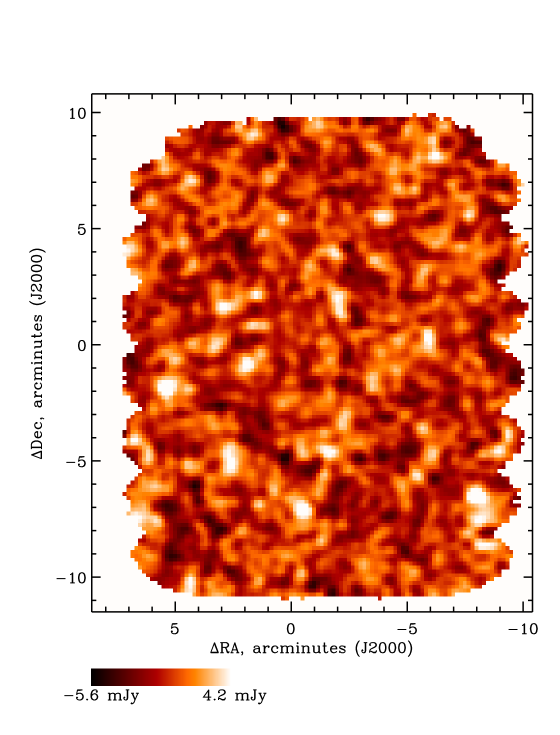
Figure 1: The Bolocam 1.1mm map of the Lockman Hole region. Only the good coverage region is shown; the rest of the map has been masked off. The map is centered on RA (J2000) $10^{\rm h}52^{\rm m}08.82^{\rm s}$ and Dec (J2000) $+57^{\circ}21^{\prime}33.8^{\prime\prime}$. The map pixels are $10^{\prime\prime}\times 10^{\prime\prime}$ and the RMS is 1.4 mJy; the color scale ranges from $-5.6$ to $+4.2$ mJy.

The measured $P(D)$ of an astronomical map is simply the pixel distribution: the number of pixels in each flux density bin, summed over the entire map. No flux density thresholds are imposed, and the entire uniform coverage region is included. Because of the faintness of the sources in the map, we have (as in Laurent et al. , 2005) taken advantage of our knowledge of the Bolocam beam shape to optimally filter the map for point sources. This increases the effective beam size, which increases the amount of source confusion (see §4); however, the improved S/N of the sources (since optimal filtering reduces the noise level in the map) more than compensates for the worsening of source confusion. Figure 1 displays the cleaned, optimally-filtered Lockman Hole map (this is the same map presented by Laurent et al.), while Figure 2 shows the observed $P(D)$ distribution. A total of 66 bins were used, as a compromise between resolution of the distribution and the number of pixels/bin (see below). Note also that the mean has been subtracted from the map, so the peak of the distribution is nearly (but not precisely, due to the presence of sources in the map) at zero.

We need to construct theoretical $P(D)$ distributions to compare with the observed distribution, for a given choice of source model (i.e., number of sources per unit area as a function of flux density). This can be done directly for an assumed number count distribution (see e.g.,  Takeuchi & Ishii, 2004) provided the beam shape and the noise are well characterized, but there are two complications for the Lockman Hole data: the shape of the optimal filter is not analytic, and even within the uniform coverage area, there are fluctuations in the number of observations per pixel, which translate to variations in the noise level (at about the 6% level, prior to optimal filtering); see Figure 1 of Laurent et al.  (2005).

We have therefore taken an alternate approach, in which we construct simulated maps from which we calculate the $P(D)$ distribution directly, just as for the actual data. The source distribution in all cases is a featureless power-law, with differential number count distribution

$$n(S)=n_{o}S^{-\delta}\ {\rm mJy^{-1}\ deg^{-2}}$$ (5)

where $S$ is the source peak flux density (in mJy). For all of the simulations the flux density range used was 0.1 to 10 mJy; the lower limit is small enough compared to the RMS noise that varying it has no significant effect on the results (decreasing it merely increases the DC level of the map, which is set to zero in any case), while the upper limit simply ensures that there are no sources much brighter than any present in the Lockman Hole. (In fact, because of the steepness of most of the source distributions considered, the results are generally independent of the choice of maximum flux, for any value larger than this.) The sources are added to a blank map with peak flux densities randomly drawn from the above power-law, as gaussian sources with size matched to the pointing-smeared Bolocam beam FWHM of $36.7^{\prime\prime}$. The simulated map pixels are fixed at $10^{\prime\prime}\times 10^{\prime\prime}$, as in the real map shown in Figure 1. The sources are uniformly randomly placed (i.e., zero spatial correlation; note that strong clustering of the sources will affect the resulting $P(D)$ distribution: Barcons, 1992; Takeuchi & Ishii, 2004) over an area larger than the final map, so that sources can fall only partially within the map.

In order to match the Bolocam observations, the noise is calculated using the measured PSD from the Lockman jackknife maps, which contain no source signal (Laurent et al. , 2005): a white noise realization is constructed in Fourier space, then multiplied by the jackknife PSD and normalized to produce the correct noise RMS (see discussion in §5.2 of Laurent et al. , 2005). In other words, the simulated noise map is constructed so that it has, on average, both the same RMS and the same power as a function of spatial frequency as the actual noise in the Lockman Hole map. The resulting noise map is then corrected for the coverage variations, and added to the source map. Although the PSD of the same jackknife map was used for all of the simulations, we verified that the difference between the PSDs of different jackknife maps is no larger than the differences produced by using independent white noise realizations multiplied by the same PSD, the procedure used here.

Since there are only about 12,000 pixels in the good coverage region, the effect of shot noise (in both the source and noise contributions) in the simulations is substantial. To eliminate this as a source of uncertainty, we initially generated between 50 and 150 independent realizations for each choice of source power-law: in each realization the sources are randomly drawn from the specified power-law, while a random realization of the noise map is generated as described above. The pixel flux density distribution for each of these maps is then calculated, and these are averaged together to produce the theoretical $P(D)$.

To analyze the fluctuations in the real data, we have carried out a maximum likelihood analysis to compare the observed pixel distribution with the predicted $P(D)$ from the simulations for a broad range of power-law models. As discussed by Friedmann & Bouchet (2004), as long as we ensure that the number of pixels in each bin is large, so that the Poisson distribution of the number of pixels per bin is closely approximated by a Gaussian, and that there are negligible correlations between pixel bins, then maximizing the likelihood function is equivalent to minimizing

$$Q^{2}=\sum_{i=1}^{N_{bins}}\left({{p_{i}-\mu_{i}}\over\sqrt{\mu}_{i}}\right)^{2}$$ (6)

where $p_{i}$ is the number of pixels within flux bin $i$ in the Lockman Hole data and $\mu_{i}$ is the expected number of pixels in the bin as predicted by the assumed noise-convolved model. In other words, if the above assumptions are satisfied, then $Q^{2}$ is a good approximation to $\chi^{2}$, and minimizing $Q^{2}$ is equivalent to maximum likelihood estimation. The choice of 66 bins over the range $-4.5$ to $+4.8$ mJy was made as a compromise between resolving the distribution and keeping the number of pixels per bin large enough so that the above assumption is reasonably well satisfied over most of the range. In the actual calculation of $Q^{2}$, any bins with fewer than 10 pixels in either the observed or predicted $P(D)$ were not included; the smallest number of bins actually used was 56, and was typically 58 or 59. Both the best-fit values and the errors on the derived number-count parameters were derived by directly mapping out $\chi^{2}$ space by variation of the model parameters. Once the general shape of the $\chi^{2}$ distribution was established, we ran a new set of models covering the interesting region of parameter space, with 200 realizations of each model.

In Figure 3 (left-hand panel) we show the Lockman $P(D)$ from Figure 2 again, overplotted with the theoretical $P(D)$ produced by averaging 100 realizations of a noise-only simulation. The obvious discrepancies between the two distributions - the higher peak and narrower width of the noise-only $P(D)$ - are simply a reflection of the presence of signal in the Lockman map. In the right-hand panel, we plot the Lockman $P(D)$ again, now overplotted with the simulated $P(D)$ for the best-fitting model, which has $\delta=2.7$ and $n_{o}=1595$ mJy^-1 deg^-2. The reduced chi-square for this model is $\chi_{\nu}^{2}=0.90$ ($\chi^{2}=51.5$ for 57 degrees of freedom); for reference, $\chi_{\nu}^{2}=9.3$ for the noise-only realization.

The number of sources per beam at the 1 mJy level is only about 0.1; it is the noise level in the map, rather than the density of sources, that limits the flux density we can probe with the fluctuation analysis. Our best-fit model implies that Bolocam would reach the $\sim 1$ source per beam level at $S_{\nu}\approx 0.3$ mJy. We also note that, although we could in principle have fit a more complicated model (e.g., a broken power-law) to the data, the goodness of fit of the best-fitting model is quite high, with a 68% probability (for 59 bins - 2 model parameters = 57 degrees of freedom) that $\chi^{2}$ would exceed this value by chance. Hence there is no compelling reason for fitting a more complex model.

In Figure 4 we show the $\chi^{2}$ map of the power-law model parameter space. The abscissa is the power-law index, $\delta$; for the ordinate we have used the normalization $N(>1{\;\rm mJy})$, the number of sources per square degree with peak flux density greater than or equal to 1 mJy (i.e., the integral number count distribution). This is related to $n_{o}$ by

$$n_{o}=(\delta-1)N(>S)S^{\delta-1}$$ (7)

where $S$ is the peak flux density. The contours are $\Delta\chi^{2}$ for joint confidence limits on $\delta$ and $N$ of $68\%$, $95.4\%$, and $99.7\%$, labeled with $1$ for $\Delta\chi^{2}=2.3$, $2$ for $\Delta\chi^{2}=6.17$, and $3$ for $\Delta\chi^{2}=11.8$. The location of the minimum is marked by a cross, with $N(>1{\;\rm mJy})\simeq 940$ deg^-2. To further reduce the noise, the contours have been mildly smoothed by re-gridding via Delaunay triangulation. The 95% confidence limits on $\delta$ and $N$ (marginalizing over $N$ and $\delta$, respectively) are $\delta=2.7$$\buildrel{\scriptscriptstyle+0.18}\over{\scriptscriptstyle-0.15}$ , $N=940$$\buildrel{\scriptscriptstyle+50}\over{\scriptscriptstyle-140}$ deg^-2, respectively. The equivalent confidence region for $n_{o}$ is $n_{o}=1595$$\buildrel{\scriptscriptstyle+85}\over{\scriptscriptstyle-238}$ mJy^-1 deg^-2.

3 Comparison with the Lockman Hole Point Source Results

As noted above, Laurent et al.  (2005) determined the best-fitting number counts in the observed Lockman Hole region by identifying point sources, carrying out extensive simulations to determine the effects of flux bias and completeness, then performing a maximum likelihood analysis to constrain the allowed number counts (assumed to be a power-law). Since only source candidates above $3\sigma$ were considered, this analysis only provides information on the number counts above an observed flux density $S_{\nu}\approx 4$ mJy. Hence the only fair way to compare the results from this paper with the Laurent et al.  (2005) results is to convert the $P(D)$ number count constraints from 1 mJy to 4 mJy. This requires scaling the normalization by a factor of $4^{1-\delta}$ (see equation [7] above). We also need to rescale the Laurent et al.  (2005) results, since their normalization parameter $A$ (chosen to reduce the degeneracy between $n_{o}$ and $\delta$ when only a small range in flux density is available) is related to the integral number counts by $N(>4\;{\rm mJy})=4A/(\delta-1)$ for $\delta>1$.

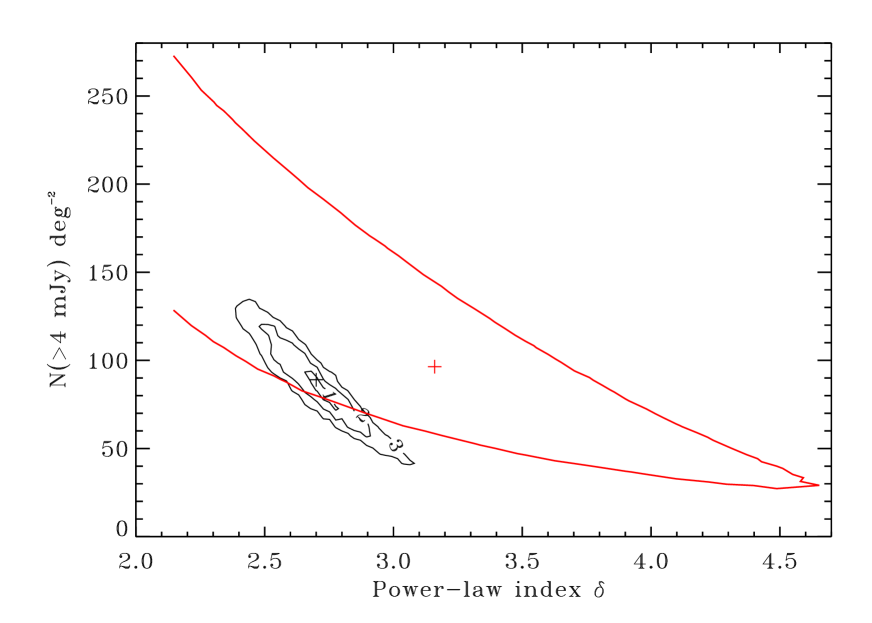
Figure 5: As Figure 4, but for the integral 4 mJy counts, for comparison with results of Laurent et al.  (2005). The minimum value of $\chi^{2}$ (marked by a cross) is located at $\delta\simeq 2.7$, $N(>4\;{\rm mJy})\simeq 88.9\ {\rm deg}^{-2}$. The joint confidence regions for $\delta$ and $N$ are labelled as in Figure 4. Shown in red are the joint $68\%$ confidence region determined by Laurent et al.  (2005) (this is truncated due to the prior assumption that $\delta>2$) and their derived minimum, at $\delta=3.2$ and $N(>4\;{\rm mJy})\simeq 96.3\ {\rm deg}^{-2}$. The agreement between the two methods is very good.

In Figure 5 we show the re-scaled $P(D)$ results (note that the effect of this correction is to suppress (in $N$) the higher-$\delta$ part of the distribution and magnify the low-$\delta$ end, compared to the 1 mJy counts shown in Figure 4), with the same contours as in Figure 4. The minimum is located at $N(>4\;{\rm mJy})\simeq 88.9$ deg^-2. Also plotted, in red, are the joint $68\%$ $N$-$\delta$ contour for the point source-derived number counts and the location of the minimum (also in red) at $N(>4\;{\rm mJy})\simeq 96.3$ deg^-2. Clearly, the results from both analyses are in good agreement with one another: the $P(D)$ minimum lies within the 68% confidence contour from the number-count analysis of Laurent et al.  (2005). The 4 mJy normalizations differ by less than $10\%$. The smaller value of the power-law index preferred by the fluctuation analysis is undoubtedly a consequence of the greater dynamic range in flux density that is included, since very few data are discarded. Because of the steepness of the allowed power-laws ($\delta\sim 2.5$ - 3), a factor of four decrease in flux density results in an order of magnitude increase in the integrated number of sources, which accounts for the much smaller errors on $N$ and $\delta$ produced by the fluctuation analysis.

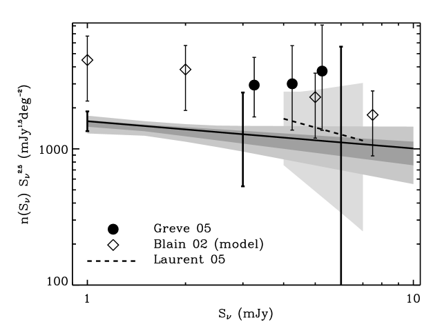
Figure 6: Observed and theoretical differential number counts at $\lambda\simeq 1.1$mm. The counts have been scaled by $S^{2.5}$. The solid line shows the best-fit model from the fluctuation analysis of this paper; the dark gray and light gray shaded regions show the 68% and 95% confidence limits. The dashed line above 4 mJy is the best-fit model from the number-count analysis of Laurent et al.  (2005), while the very light gray region displays their 68% confidence region. The filled circles are derived from the 1.2mm MAMBO observations of Greve et al.  (2004); the error bars indicate the Poisson two-sided 95% confidence limits, calculated for the observed area (370 square arcminutes) and scaled to one square degree. The open diamonds are the model number counts of Blain et al.  (2002) at 1, 2, 5, and 7.5 mJy (we have plotted only a few points rather than the full range simply for clarity); the error bars have been taken to be a factor of two (Blain, 2004). The thick error bars plotted on the $P(D)$ results at 1, 3 and 6 mJy show the two-sided 95% confidence Poisson errors on the differential number counts assuming that the best-fit model is correct. These errors were derived for a Lockman Hole-sized field and scaled to one square degree.

In Figure 6 and 7 we show our derived number counts together with the Laurent et al.  (2005) number counts, as well as all of the other directly comparable observed and theoretical number counts (discussed below). Figure 6 plots the differential number counts, while 7 shows the cumulative number counts. The differential counts are much to be preferred since they require no assumptions about the source distribution at fluxes higher than have been observed; furthermore, the integral counts tend to obscure any structure in the number count distribution. To facilitate comparison with other work, we nonetheless show the cumulative counts as well.

The differential number counts in Figure 6 have also been multiplied by a factor of $S^{2.5}$, to remove the scaling expected for a Euclidean universe of uniform sources; since the best-fit slope is $-2.7$, the model is nearly flat in this representation. The solid line shows the best fit model from the $P(D)$ analysis; the dark gray and light gray shaded regions show the 68% and 95% confidence regions, respectively. The dashed line above 4 mJy shows the Laurent et al. counts, while the very light gray region shows the 68% confidence region for their number counts. The agreement between the point source-derived number counts of Laurent et al.  (2005) and the number counts produced by the fluctuation analysis of this paper is excellent, but the fluctuation analysis provides much tighter constraints and extends to much lower flux densities. Also plotted (the thick error bars at 1, 3 and 6 mJy) are the two-sided 95% confidence Poisson errors on the number counts; these have been derived for a Lockman Hole-sized field and then scaled to one square degree.

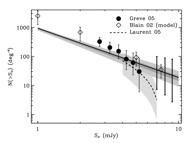
Figure 7: Observed and theoretical integrated number counts at $\lambda\simeq 1.1$mm. The solid line shows the best-fit model from the fluctuation analysis of this paper; the dark gray and light gray shaded regions show the 68% and 95% confidence limits. The dashed line above 4 mJy is the best-fit model from the number-count analysis of Laurent et al.  (2005), while the very light gray region displays their 68% confidence region. The filled circles are the 1.2mm MAMBO number counts derived by Greve et al.  (2004); the error bars are two-sided 95% Poisson confidence limits. The open diamonds are the model number counts of Blain et al.  (2002) at 1, 2, 5, and 7.5 mJy (we have plotted only a few points rather than the full range simply for clarity); the error bars have been taken to be a factor of two (Blain, 2004). The thick error bars plotted on the $P(D)$ results at 7, 8 and 9 mJy show the two-sided 95% confidence Poisson errors on the integrated number counts assuming that the best-fit model is correct. As in Figure 6, these errors were derived for a Lockman Hole-sized field and scaled to one square degree.

Figure 7 plots in the same fashion the cumulative number counts. The apparent discrepancy between the $P(D)$ results and the Laurent et al. results as $S_{\nu}$ approaches 7 mJy is a consequence of the imposition of a high-flux cutoff of 7.4 mJy in the latter analysis, in consequence of the absence of any sources brighter than 7 mJy. To emphasize that this apparent discrepancy is not significant, in Figure 7 we also plot the Poisson errors on the best-fit number counts for 7, 8 and 9 mJy; as for the differential number counts, these have been calculated for a field the size of the Lockman Hole and then scaled to one square degree. As was also evident in Figure 6, the Lockman Hole field is simply not large enough in area to provide strong constraints on the number density of sources at flux densities significantly in excess of 7 mJy.

4 Discussion and Implications

The Bolocam Lockman Hole observations (Laurent et al. , 2005) have provided some of the first significant observational constraints on the number counts of high-redshift galaxies at $\lambda\approx 1.1$mm. In this paper we have taken advantage of the extremely uniform noise level of this data set and performed a fluctuation analysis. Since it is not necessary to extract point sources for this analysis, we are able to probe the number count distribution to lower flux density levels than in the previous paper, and provide substantially tighter constraints on the slope and amplitude of the number counts at this wavelength than any previous work.

The important results in this paper are presented in Figures 4, 5, 6 and 7. The best-fitting power-law number count model has an index $\delta=2.7$$\buildrel{\scriptscriptstyle+0.18}\over{\scriptscriptstyle-0.15,}$ a differential number density at 1 mJy $n_{o}\simeq 1595$$\buildrel{\scriptscriptstyle+85}\over{\scriptscriptstyle-238}$ mJy^-1 deg^-2, and an integrated number density $N(>1\;{\rm mJy})\simeq 940$$\buildrel{\scriptscriptstyle+50}\over{\scriptscriptstyle-140}$ deg^-2 (95% confidence limits).

At present there are few other observational results or theoretical predictions for the 1.1mm number counts to which our results can be compared. We have overplotted the relevant observational and theoretical values on our derived number counts in Figures 6 and 7.

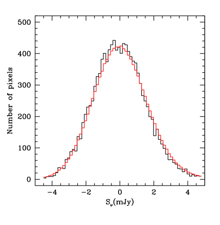
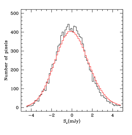
Figure 8: (left): The Lockman Hole $P(D)$ distribution from Figure 2 (black), overplotted with the pixel distribution produced by 200 realizations of the best-fitting model ($\delta=3.2$) using the MAMBO (Greve et al. , 2004) normalization (red). This model has $\chi^{2}=77.3$ (for 57 degrees of freedom) compared to $\chi^{2}=51.5$ for the best-fitting model from the fluctuation analysis (see Figure 3). (right): The same as Figure 8a, for the Blain et al.  (2002) prediction of $\delta=3.1$, $N(>1\;{\rm mJy})=2480$ deg^-2. This model has $\chi^{2}=133$.

The most direct observational comparison is with the 1.2mm MAMBO results of Greve et al.  (2004). We have used the source catalogs for the Lockman Hole and ELAIS N2 fields presented in that paper, along with the completeness and bias corrections they adopted (kindly provided by T. Greve) to calculate the differential counts for the combined fields. The counts were calculated for 1 mJy-wide bins centered at 3.25, 4.25, and 5.25 mJy. The number counts and the 95% two-sided Poisson error bars, scaled to one square degree, are plotted as the solid circles in Figure 6. The slopes are essentially identical, but the normalization implied by the MAMBO number counts is higher than our best-fit value: the MAMBO counts are higher by factors of 2.3, 2.5, and 3.3 at 3.25, 4.25, and 5.25 mJy, respectively. We show the Lockman histogram together with the best-fitting model ($\delta\approx 3.2$) with the MAMBO 2.75 mJy normalization in Figure 8a; this model has $\chi^{2}=77.3$ for 57 degrees of freedom, and hence is statistically a much worse fit than our result. However, the discrepancy between the two results is arguably not significant, because the errors in the normalizations are dominated by the systematic uncertainties in the flux densities.

The flux bias correction determined by Laurent et al.  (2005) (note that this correction does not include the effects of Eddington bias, which are automatically incorporated into the simulations) is $\epsilon=0.71$$\buildrel{\scriptscriptstyle+0.08}\over{\scriptscriptstyle-0.10}$ ($90\%$ errors). The uncertainty on the bias correction translates directly into a systematic uncertainty in the number counts, since the normalization $n_{o}\propto\epsilon^{-\delta}$. For $\delta\approx 2.5$ - 3, the resulting uncertainty in $n_{o}$ is approximately a factor of two. Obviously, this systematic error term is much larger than the statistical uncertainties on $n_{o}$ resulting from the $P(D)$ analysis, and is larger than the shot noise (Poisson) errors for $S_{\nu}\;\lower 2.15277pt\hbox{$\buildrel<\over{\sim}\ $}3$ mJy. The true uncertainty on $n_{o}$ is entirely dominated by how well the absolute calibration can be established. Similar considerations apply, of course, to any observational determination of the number counts, such as the (Greve et al. , 2004) results; they quote an absolute calibration uncertainty of 20%. At the best-fit power-law index $\delta=2.7$, the 90% systematic errors imply that $n_{o}$ could be 50% larger, or 25% smaller, than our quoted value. An error in the absolute calibration affects only the normalization, $n_{o}$ (or $N$), and hence will affect the vertical position and shape of the confidence regions (since it is a $\delta$-dependent term), but not the location or extent of these regions along the $\delta$-axis. Hence, given the magnitude of the systematic uncertainties in both the Bolocam and MAMBO data sets, the number count results appear to be consistent.

Also plotted in Figure 6 are the model differential number counts of Blain et al.  (2002) (open diamonds). The model predicts a slope $\delta\simeq 3.1$ and a differential number count $n(S)=4500$ mJy^-1 deg^-2 at 1 mJy, nearly a factor of three above our best-fit value and (formally) many $\sigma$ away from the $P(D)$ minimum; the resulting histogram is shown with the Lockman data in Figure 8b. Although Blain et al.  (2002) do not report uncertainties on the model predictions, allowing for a reasonable factor of two error on the number counts (Blain, 2004) still places the Blain et al.  (2002) prediction more than $5\sigma$ from our best-fit result. Because of the steeper predicted slope compared to the value we derive, the discrepancy decreases with increasing flux density: at 7.5 mJy our result and the Blain et al.  (2002) prediction are within $\simeq 10\%$ of one another. As with the comparison with the MAMBO counts, the magnitude of the systematic flux uncertainties makes it possible to reconcile the model normalization (within the errors) with the data. Both the $P(D)$ results and the MAMBO data clearly suggest a shallower slope than the Blain et al.  (2002) prediction.

In Figure 7 we plot the same data sets and model predictions, but now in the form of the cumulative number counts. This is potentially a very misleading plot. Note that, while in the differential number count plot of Figure 6 the MAMBO data points always lie above our best-fit results from the $P(D)$ analysis (i.e., the MAMBO normalization is higher), in the cumulative number count plot the MAMBO number counts decline to match the $P(D)$ results at 4.25 mJy and drop below them (although not significantly) at higher flux densities.

The reason for this apparent discrepancy between the two plots lies in the presence of an effective cut-off in the MAMBO number counts: there are no sources (after bias correction) with fluxes that exceed 5.7 mJy, and the counts are derived simply by summing over the observed sources (including a correction for completeness). Hence the apparent convergence of the MAMBO counts to the Bolocam counts with increasing flux density is illusory; it is the result of comparing the cumulative number counts from the fluctuation analysis, which have been calculated by extrapolating the best-fit model to arbitrarily high fluxes, with the MAMBO counts. A fair comparison of the two would require that we impose a cut-off on the $(PD)$ result as well, in which case the cumulative $P(D)$ results would also decline at higher flux densities, leading to a more or less constant ratio between our number counts and the Greve et al counts, as is seen in the differential number counts. This behavior is also seen for the Lockman Hole point-source-derived number counts, for which the maximum-likelihood fit had a cut-off of 7.4 mJy imposed (see discussion at the end of §3).

We can use our best-fitting number count model to estimate the fraction of the 1.1mm background radiation that has been resolved into sources. Integrating from 1 to 10 mJy (the range included in the fluctuation analysis), we obtain

$$I_{\nu}=5.8\times 10^{-23}\;{{\rm W\ m}^{-2}{\rm\ Hz}^{-1}{\rm\ sr}^{-1}}$$ (8)

which is $7\%$ of the 1.1mm background as determined by FIRAS (Fixsen et al. , 1998). This is about twice the value obtained directly from the Bolocam Lockman Hole number counts, and half the result of integrating the best-fitting maximum-likelihood number count model from Laurent et al.  (2005). If we extrapolate our best-fit result to below 1 mJy, we find that at the Bolocam one-source-per-beam level of about 0.3 mJy approximately 20% of the 1.1mm background would be resolved; at 0.1 mJy this would rise to 45%.

The optimal design of future mm-wave surveys depends on precisely what question one wishes to address. As pointed out by Laurent et al.  (2005) and discussed in more detail above, the Bolocam Lockman Hole survey places almost no constraints on the bright end of the number count distribution, simply because the surveyed area was not large enough to detect rare, bright objects. A survey aimed at probing this end of the luminosity function should cover more area, at the cost of reduced depth (for a reasonable amount of observing time). Such a survey is currently being carried out with Bolocam as part of the COSMOS survey. On the other hand, in order to study the sources that dominate the cosmic background at 1.1mm, a deeper survey is required. As noted above (§2), the analysis in this paper suggests that even at the 1 mJy level, we are just barely touching the confusion limit, indicating that a deeper survey would be worthwhile. As with the present data set, a survey with very uniform noise is highly desirable for this analysis, since it makes it possible to carry out a reliable fluctuation analysis in addition to extraction of point sources. As discussed above, however, systematic uncertainties in flux calibration are likely to remain as the major source of uncertainty in determining the number counts of sub/mm galaxies and related quantities, such as the fraction of the millimeter background that has been resolved.

Appendix A Effect of Optimal Filtering on the Pixel Distribution

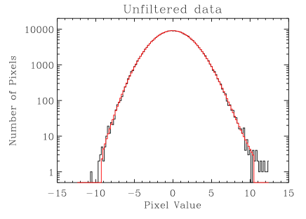
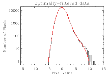
Figure 9: (left): Pixel distribution of a simulated map (black), using the the best-fitting model from the fluctuation analysis, with white noise with an rms of 2.3 mJy per pixel. Overplotted in red is the theoretical $P(D)$ distribution; this depends only on the assumed number count model, the noise level, and the number of pixels in the map. The beam is assumed to be a Gaussian with a FWHM of 3 pixels, and the map is 512 pixels on a side. (see Figure 3). (right): The same as Figure 9a, but for the optimally-filtered map. In this case the optimal filter was assumed to be identical to the beam. The map is now 504 pixels on a side, since pixels close to the map boundaries must be discarded to avoid edge effects in filtering. The rms noise per pixel has been reduced to 1 mJy by filtering, with the result that the signal in the map is far more prominent. As in Figure 9a, the theoretical $P(D)$ distribution precisely matches the “observed” distribution, except for the most extremal bins, which are affected by shot noise; these are discarded in our analysis.

As noted in §2 of the text, since optimal filtering is a linear operation, it will have no effect on the fluctuation analysis. To demonstrate this, in Figure 9a we show (in black) the pixel distribution of a simulated map; the x-axis is in mJy. The number count model that was used has the same amplitude and slope as derived from the P(D) analysis in this paper, but we have used a larger map area ($512^{2}$ pixels, with 3 pixels per beam FWHM) to reduce the shot noise for the sake of illustration. The noise (which is purely white in this case, also for convenience) has an rms per pixel of 2.3 mJy. This map has not been optimally-filtered; the source contribution is just barely visible in this representation as an excess on the positive side of the distribution. Overplotted in red is the theoretical P(D) distribution predicted for this model; this depends only on the assumed number count model and the noise distribution, and has been binned in the same way as the observed pixel distribution.

For simplicity, we have taken the optimal filter to be identical to the beam. Figure 9b, labelled ”Optimally-filtered data”, plots the same two quantities, but now for the filtered map. The signal is far more prominent in this plot, because of the improvement in signal to noise of the map due to the optimal filtering. The rms of the noise has been reduced by a factor of 2.3. (We don’t gain as large a reduction in the Lockman Hole data, because of the $1/f$ noise remaining in the map even after cleaning.) Shown in red again is the theoretical $P(D)$ distribution. This is again the predicted value, not a fit: the only thing that has been altered in calculating this distribution is the RMS of the noise and the number of sources per beam (since the PSF of sources in the filtered map is larger by root two as a result of the convolution), as well as a slight reduction in the number of pixels (since pixels close to the map edge must be discarded when the map is filtered). There is precise agreement between the “observed” and predicted distibutions, except at the most extremal bins, where the effects of shot noise are becoming large; this is why we discard such bins in the analysis.

Figure 2: Pixel flux density distribution of the Lockman Hole map shown in Figure 1. There are 66 bins in flux density, extending from $-4.5$ to $+4.8$ mJy.

Fig. 3. — Left: The Lockman Hole $P(D)$ distribution from Figure 2 (black), overplotted with the pixel distribution produced by 100 realizations of a noise-only map (red). The marked discrepancies between the two are a consequence of the signal in the actual map. Right: The actual $P(D)$ as in the left panel, now overplotted (in red) with the theoretical $P(D)$ produced by the best-fitting power-law model, with $\delta=2.7$ and $n_{o}=1595$ mJy^-1 deg^-2. This model has $\chi^{2}=51.5$, for 59 degrees of freedom.

Figure 4: Joint confidence limits for fit of power-law number count models to the Lockman Hole $P(D)$ distribution. The abscissa is the index of the differential power-law, while the ordinate is the normalization, taken to be number of sources per square degree with peak flux densities greater than or equal to 1 mJy. The minimum value of $\chi^{2}$, $\chi^{2}=51.5$, marked by a cross, is located at $\delta\simeq 2.7$, $N(>1\;{\rm mJy})\simeq 938\ {\rm deg}^{-2}$; this corresponds to a normalization for the differential number counts $n_{o}=1595$ mJy^-1 deg^-2. The joint confidence regions for $\delta$ and $N$ are labeled with the values of $\Delta\chi^{2}$ as follows: $1$ for $\Delta\chi^{2}=2.3$, $2$ for $\Delta\chi^{2}=6.17$, and $3$ for $\Delta\chi^{2}=11.8$. The contours have been mildly smoothed by re-gridding onto a uniform grid to further reduce the noise.

References

- Barcons (1992) Barcons, X. 1992, ApJ, 396, 460
- Blain (2004) Blain, A. W. 2004, priv. comm.
- Blain et al. (2002) Blain, A. W., Smail, I., Ivison, R. I., Kneib, J. -P., & Frayer, D.T. 2002, Phys. Rep., 369, 111
- Bond et al. (2005) Bond, J.R. et al. 2005, ApJ, in press (astro/ph0205386)
- Condon (1974) Condon, J. J. 1974, ApJ, 188, 279
- Fixsen et al. (1998) Fixsen, D.J., Dwek, E., Mather, J.C., Bennett, C.L., & Shafer, R.A. 1998, ApJ, 508, 123
- Friedmann & Bouchet (2004) Friedmann, Y., & Bouchet, F. 2004, MNRAS, 348, 737
- Greve et al. (2004) Greve, T. R., Ivison, R. J., Bertoldi, F., Stevens, J. A., Dunlop, J. S., Lutz, D., & Carilli, C. L. 2004, MNRAS, 354, 779
- Guiderdoni et al. (1997) Guiderdoni, B., Bouchet, F.R., Puget, J.-L., Lagache, G., & Hivon, E. 1997, Nature, 390, 257
- Hauser & Dwek (2001) Hauser, M. G., & Dwek, E. 2001, ARA&A, 39, 249
- Kashlinsky (2005) Kashlinsky, A. 2005, Phys. Rep., 409, 361
- Lagache, Dole, & Puget (2003) Lagache, G., Dole, H, & Puget, J.-L. 2003, A&A, 338, 555
- Laurent et al. (2005) Laurent, G.T., et al. 2005, ApJ, 623, 742
- Masi et al. (2001) Masi, S. et al. 2001, ApJ, 553, L93
- Puget (1996) Puget, J.-L., et al. 1996, A&A, 308, L5
- Scheuer (1957) Scheuer, P. A. G. 1957, Proc. Camb. Philos. Soc., 53, 764
- Sandell (1994) Sandell, G. 2004, MNRAS, 271, 75
- Scheuer (1974) Scheuer, P. A. G. 1974, MNRAS, 166, 329
- Scott et al. (2002) Scott, S.E., et al. 2002, MNRAS, 331, 817
- Smail et al. (2002) Smail, I., Ivison, R.J., Blain, A.W., & Kneib, J.-P. 2002, MNRAS, 331, 495
- Stompor et al. (2001) Stompor, R. et al. 2001, ApJ, 561, L7
- Takeuchi & Ishii (2004) Takeuchi, T. T., & Ishii, T.T. 2004, ApJ, 604, 40
- White (1992) White, M. 1992, PhysRevD, 46, 4198
- Zhang, Pen & Wang (2002) Zhang, P., Pen, U.-L., & Wang, B. 2002, ApJ, 577, 555