The Number Density of Intermediate and High Luminosity Active Galactic Nuclei at $z\sim 2-3$

Abstract

We use the combination of the 2 Ms Chandra X-ray image, new $J$ and $H$ band images, and the Spitzer IRAC and MIPS images of the Chandra Deep Field-North to obtain high spectroscopic and photometric redshift completeness of high and intermediate X-ray luminosity sources in the redshift interval $z=2-3$. We measure the number densities of $z=2-3$ active galactic nuclei (AGNs) and broad-line AGNs in the rest-frame $2-8$ keV luminosity intervals $10^{44}-10^{45}$ and $10^{43}-10^{44}$ ergs s^-1 and compare with previous lower redshift results. We confirm a decline in the number densities of intermediate-luminosity sources at $z>1$. We also measure the number density of $z=2-3$ AGNs in the luminosity interval $10^{43}-10^{44.5}$ and compare with previous low and high-redshift results. Again, we find a decline in the number densities at $z>1$. In both cases, we can rule out the hypothesis that the number densities remain flat to $z=2-3$ at above the $5\sigma$ level.

1. Introduction

Low-redshift hard X-ray luminosity functions have been well determined from the combination of highly spectroscopically complete deep and wide-area Chandra X-ray surveys. At $z<1.2$, the hard X-ray luminosity functions for active galactic nuclei (AGNs) of all spectral types and for broad-line AGNs alone are both well described by pure luminosity evolution, with $L_{\ast}$ evolving as $(1+z)^{3.2}$ and $(1+z)^{3.0}$, respectively (Barger et al. 2005). AGNs decline in luminosity by almost an order of magnitude over this redshift range.

Barger et al. (2005) compared directly their broad-line AGN hard X-ray luminosity functions with the optical QSO luminosity functions from Croom et al. (2004) and found that the bright end luminosity functions agree extremely well at all redshifts. However, the optical QSO luminosity functions do not probe faint enough to see the downturn in the broad-line AGN hard X-ray luminosity functions at low luminosities and may be missing some sources at the very lowest luminosities to which they probe.

The Croom et al. (2004) pure luminosity evolution is slightly steeper than that of Barger et al. (2005), but within the uncertainties, the two determinations are consistent over the $z=0-1.2$ redshift interval. To investigate whether pure luminosity evolution continues to hold at higher redshifts, Barger et al. (2005) used the Croom et al. (2004) evolution law (which was fitted over the wider redshift range $z=0.3-2.1$) to correct all of their broad-line AGN hard X-ray luminosities to the values they would have at $z=1$. They then computed the broad-line AGN hard X-ray luminosity functions over the wide redshift intervals $z=0.2-0.7$, $0.7-1.5$, and $1.5-2.5$. Barger et al. (2005) found that the lower redshift luminosity functions matched each other throughout the luminosity range, while the highest redshift luminosity function matched the lower redshift functions only at the bright end, where the optical QSO determinations were made. They therefore concluded that there are fewer intermediate X-ray luminosity broad-line AGNs in the $z=1.5-2.5$ redshift interval, and hence that the pure luminosity evolution model cannot be carried reliably to the higher redshifts. This was consistent with other analyses made of less complete samples of all spectral types together, which had found evidence for peaks and subsequent declines in the number densities of both intermediate-luminosity (e.g., Cowie et al. 2003; Barger et al. 2003a; Hasinger 2003; Fiore et al. 2003; Ueda et al. 2003) and high-luminosity (Silverman et al. 2005) sources, with the intermediate-luminosity sources peaking at lower redshifts than the high-luminosity sources.

Recently, Nandra et al. (2005; hereafter, N05) have questioned the evidence for a decline in the number densities of intermediate-luminosity AGNs at $z>1$. By combining deep X-ray data with the Lyman break galaxy (LBG) surveys of Steidel et al. (2003), they argue that the number densities of intermediate-luminosity AGNs are roughly constant with redshift above $z=1$.

Only with extremely deep X-ray data and highly complete redshift identifications can we address the above controversy about a decline. In this paper, we measure the $z=2-3$ number densities of both high and intermediate X-ray luminosity sources in the 2 Ms Chandra Deep Field-North (CDF-N). In addition to our highly complete spectroscopic redshift identifications, we also use the recently released Spitzer Great Observatories Origins Deep Survey-North IRAC and MIPS data, in combination with deep $J$ and $H$ band data obtained from the ULBCAM instrument on the University of Hawaii’s 2.2 m telescope, to estimate accurate infrared (IR) photometric redshifts for the X-ray sources that could not be spectroscopically or optically photometrically identified. We assume $\Omega_{M}=0.3$, $\Omega_{\Lambda}=0.7$, and $H_{0}=70$ km s^-1 Mpc^-1 throughout.

2. Data

The deepest X-ray image is the $\approx 2$ Ms CDF-N exposure centered on the Hubble Deep Field-North taken with the ACIS-I camera on Chandra. Alexander et al. (2003) merged samples detected in seven X-ray bands to form a catalog of 503 point sources over an area of 460 arcmin². Near the aim point, the limiting fluxes are $\approx 1.5\times 10^{-17}$ ergs cm^-2 s^-1 ($0.5-2$ keV) and $\approx 1.4\times 10^{-16}$ ergs cm^-2 s^-1 ($2-8$ keV).

The ground-based, wide-field optical data of the CDF-N are summarized in Capak et al. (2004), and the HST ACS GOODS-N data are detailed in Giavalisco et al. (2004). The Spitzer IRAC and MIPS data are from the Spitzer Legacy data products release and are presented in Dickinson et al. (2005). The new ULBCAM $J$ and $H$ band data, which cover the whole CDF-N area to $1\sigma$ depths of $25.2$ in $J$ and $24.2$ in $H$ (these are measured in $3^{\prime\prime}$ apertures and corrected to total magnitudes), are described in Trouille et al. (2005). All magnitudes in this paper are in the AB system. Most of the spectroscopic redshifts for the X-ray sources are from Barger et al. (2002, 2003b, 2005), but we also obtained some additional redshifts with the DEIMOS spectrograph on the Keck II telescope during the Spring 2005 observing season. One spectroscopic redshift ($z=2.578$) is taken from Chapman et al. (2005).

2.1. X-ray Incompleteness

We consider in our analysis two restricted, uniform, flux-limited X-ray samples. The most important consideration in choosing our soft X-ray flux limits was that there be no significant X-ray incompleteness. In Figure 2.1, we show $0.5-2$ keV flux versus off-axis radius for the full 2 Ms CDF-N X-ray sample of Alexander et al. (2003) (squares and diamonds). We use small squares to denote sources that are detected in the 2 Ms survey but not in the 1 Ms survey (Brandt et al. 2001). For the bright subsample, we consider sources in a $10^{\prime}$ radius region with fluxes above $1.7\times 10^{-15}$ ergs cm^-2 s^-1 ($0.5-2$ keV), and for the deep subsample, we consider sources in an $8^{\prime}$ radius region with fluxes above $1.7\times 10^{-16}$ ergs cm^-2 s^-1 ($0.5-2$ keV). We show these flux and radius limits with solid lines. The two subsamples comprise 160 sources, 8 of which are stars.

We can see from Figure 2.1 that the flux limits of our subsamples are well above the flux limit of the 2 Ms survey (dotted curve) at all radii, suggesting that there should be very little X-ray incompleteness in our sample. Indeed, when we consider the 160 sources in the 2 Ms exposure that lie within our two subsamples, we find that only five sources were not already detected in the 1 Ms exposure. If we were using the 1 Ms catalog in our analysis rather than the 2 Ms catalog, then this would correspond to a 3% incompleteness. With the 2 Ms exposure, we expect X-ray incompleteness to be negligible.

Figure 1.— $0.5-2$ keV flux vs. off-axis radius for the full 2 Ms CDF-N sample of Alexander et al. (2003) (squares and diamonds). The flux and radius limits of our bright and faint subsamples are denoted by the solid lines, and the 2 Ms flux limit is denoted by the dotted curve. Sources detected in the 2 Ms survey but not in the 1 Ms survey (Brandt et al. 2001) are denoted by small squares. Only five such sources lie within our subsamples. Sources with spectroscopic redshifts in the interval $z=2-3$ are denoted by large squares. Our flux and radius limits were chosen without reference to the distribution of the $z=2-3$ sources.

2.2. Redshift Interval

Having selected a highly complete X-ray sample, our next concern was that we sample the full luminosity ranges of interest without clipping out any sources. For the traditional intermediate and high X-ray luminosity cut-offs of $L_{\rm 2-8~{}keV}=10^{43}$ and $10^{44}$ ergs s^-1, this very naturally sets the redshift interval to $z=2-3$. We can see this from Figure 2, where we show rest-frame $2-8$ keV luminosity versus redshift for the CDF-N X-ray sources in our (a) bright and (b) faint subsamples. We determined the rest-frame $2-8$ keV luminosities from the observed-frame $0.5-2$ keV fluxes, assuming an intrinsic $\Gamma=1.8$ spectrum. At $z=3$, observed-frame $0.5-2$ keV corresponds to rest-frame $2-8$ keV, providing the best possible match to lower redshift data. Moreover, the $0.5-2$ keV Chandra images are deeper than the $2-8$ keV images, so using the observed-frame soft X-ray fluxes at high redshifts results in increased sensitivity. We only show the luminosities at low redshifts for illustrative purposes, since normally one would use the observed-frame $2-8$ keV fluxes to calculate the $2-8$ keV luminosities at these redshifts. The soft X-ray flux limits of our faint and bright subsamples (solid curves) correspond to rest-frame $2-8$ keV luminosities of $10^{43}$ ergs s^-1 and $10^{44}$ ergs s^-1, respectively, at $z=3$. Thus, we will not be clipping out any sources in either the $L_{\rm 2-8~{}keV}=10^{43}$ to $10^{44}$ ergs s^-1 interval in the faint subsample, or the $L_{\rm 2-8~{}keV}=10^{44}$ to $10^{45}$ ergs s^-1 interval in the bright subsample, if we choose $z=2-3$ for our analysis.

Figure 2.— Rest-frame $2-8$ keV luminosity versus redshift for the CDF-N X-ray sources in our (a) bright and (b) faint restricted subsamples. The luminosities were determined using the observed-frame $0.5-2$ keV X-ray fluxes and $K$-corrections calculated using a $\Gamma=1.8$ spectrum. Sources with spectroscopic redshifts are denoted by small solid diamonds. Broad-line AGNs are denoted by large solid diamonds. Sources with IR photometric redshifts are denoted by open squares. The eight remaining sources without spectroscopic or photometric redshifts (one in the bright subsample and seven in the faint subsample) are denoted by open circles and are shown at $z=2.5$. The solid curve in (a) shows the bright subsample $0.5-2$ keV flux limit of $1.7\times 10^{-15}$ ergs cm^-2 s^-1 in a $10^{\prime}$ radius region, and the solid curve in (b) shows the faint subsample $0.5-2$ keV flux limit of $1.7\times 10^{-16}$ ergs cm^-2 s^-1 in an $8^{\prime}$ radius region. The dotted horizontal line in (a) shows the high-luminosity interval lower limit of $10^{44}$ ergs s^-1, and the dotted horizontal lines in (b) show the intermediate-luminosity interval upper and lower limits of $10^{44}$ and $10^{43}$ ergs s^-1, respectively.

Once we have chosen our soft X-ray flux and radius limits and our redshift interval, we can plot the spectroscopically identified $z=2-3$ sources in the flux-radius plane and see how many lie in our restricted subsamples. This is shown in Figure 2.1, where we denote with large squares the sources that have been spectroscopically identified to lie in the redshift interval $z=2-3$. The soft X-ray flux and radius limits for our two subsamples were chosen without regard to this distribution, as can be seen from the figure. There are 15 sources in our two subsamples with spectroscopic redshifts in the interval $z=2-3$.

2.3. Probability of Misidentifications

Another issue we need to address is how many of the X-ray sources with detected optical/near-infrared (NIR) counterparts we may be misidentifying. Of the 160 sources in the 2 Ms exposure that lie within our two subsamples, 138 are detected above the $3\sigma$ limit of 23 in $H$. Thus, only 22 of the sources in our subsamples are not detected at the $3\sigma$ level in the NIR. By randomizing the source positions and remeasuring the $H$ band magnitudes many times, we found an 11% probability of misidentification. Thus, of the 138 sources in our subsamples with $3\sigma$ $H$ band detections, we would expect that about 15 might be contaminated by the projection of random, superposed objects.

Of the 22 sources that are not detected at the $3\sigma$ level in $H$, 11 are detected in the IRAC $3.6\mu$m band at $<23$ magnitude, with a 4% probability of misidentification based on randomized measurements. This corresponds to about one-half of a source. Of the remaining 11 sources that are not detected at $3.6\mu$m, 5 are detected at $R<25.5$, with a 10% probability of misidentification based on randomized measurements. Again, this corresponds to about one-half of a source.

Thus, in total, we have optical/NIR identifications for 154 of the 160 sources, eight of which are stars, and we expect about 16 (or just over 10%) of these to be false. Even if a large fraction of the 16 real sources suffering from random projections were in the $z=2-3$ range, which is not very likely, the correction to the number densities we derive subsequently would be small.

3. Photometric Redshifts

Barger et al. (2002, 2003b) computed photometric redshifts for the CDF-N X-ray sources using broadband galaxy colors and the Bayesian code of Benítez (2000). They only used sources with probabilities for the photometric redshift of greater than 90%, resulting in about an 85% success rate for photometric identifications. These redshifts are robust and surprisingly accurate (often to better than 8% when compared with the spectroscopic redshifts) for non–broad-line AGNs.

Figure 3.— (a) Comparison of the optical photometric redshift estimates with Bayesian probabilities $>0.90$ from Barger et al. (2003b) with the spectroscopic redshifts. (b) Comparison of the IR photometric redshift estimates from this paper with the spectroscopic redshifts. Large open squares denote broad-line AGNs.

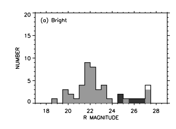
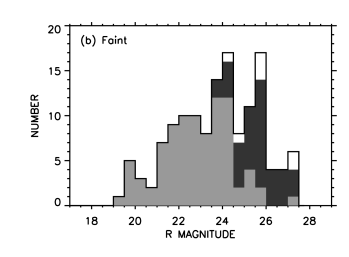
Figure 4.— Fraction of the total (open histogram) (a) bright and (b) faint restricted subsamples that are spectroscopically (light shading) and photometrically (dark shading) identified vs. $R$ magnitude. All $R>27$ sources are placed in the final magnitude bin.

Figure 5.— Bolometric flux ($\nu f_{\nu}$) vs. rest frequency for four example X-ray sources in the CDF-N sample. Solid squares show the optical (HST ACS and ground-based), near-infrared ($J$ and $H$), and mid-infrared (3.6$\mu$m, 4.5$\mu$m, 5.8$\mu$m, 8.0$\mu$m, and 24$\mu$m) measurements. Open squares denote $5\sigma$ upper limits. Curves show the average spectral energy distributions of the CDF-N X-ray sources of a given spectral class selected as templates by the IR photometric redshift estimation code (see text for details). Spectroscopic redshifts and spectral classes are used in (a) and (b), and IR photometric redshifts are used in (c) and (d).

We now have the advantage of the Spitzer IRAC $3.6\mu$m, $4.5\mu$m, $5.8\mu$m, and $8.0\mu$m data, as well as the NIR $J$ and $H$ band data, for estimating photometric redshifts. Barger et al. (2005) classified the X-ray sources into four spectral classes: absorbers (i.e., no strong emission lines [EW([OII])$<3$ Å or EW(H$\alpha+$NII)$<10$ Å]), star formers (i.e., strong Balmer lines and no broad or high-ionization lines), high-excitation (HEX) sources (i.e., [NeV] or CIV lines or strong [OIII] [EW([OIII] 5007 Å$)>3$ EW(H$\beta)$]), and broad-line AGNs (i.e., optical lines having FWHM line widths greater than 2000 km s^-1). The measured spectral energy distributions (SEDs) of the X-ray sources in each of these spectral classes turn out to be remarkably tight. Thus, we can construct templates from the average SEDs for each class and obtain an IR photometric redshift by fitting the templates to the optical through mid-infrared (MIR) data. We note that the template fitting is insensitive to the spectral class for sources without strong AGN signatures.

In Figure 3, we compare both (a) the optical photometric redshifts from Barger et al. (2003), and (b) our new IR photometric redshifts with the spectroscopic redshifts. Both photometric redshift techniques tend to fail on some of the broad-line AGNs (large open squares), but, fortunately, broad-line AGNs are straightforward to identify spectroscopically, even in the so-called redshift “desert” at $z\sim 1.5-2$, and nearly all of the CDF-N X-ray sources have now been spectroscopically observed. While the Bayesian optical photometric redshift technique gives slightly tighter values at low redshifts due to the presence of strong spectral features and breaks in the templates from Coleman, Wu, & Weedman (1988) and Kinney et al. (1996), it does not do so well on the $z>2$ sources. In our subsequent analysis, we adopt the more robust IR photometric redshifts when a spectroscopic redshift is not available. In Figure 4, we show histograms of the spectroscopic (light shading) and IR photometric (dark shading) redshift identifications versus $R$ magnitude for the sources in our (a) bright and (b) faint subsamples.

The photometric redshifts not only tell us which of the spectroscopically unidentified sources are likely to have redshifts within the $z=2-3$ redshift interval, but they also enable us to remove contaminants that are really at lower redshifts. In Figure 5, we show four example measured X-ray source SEDs (solid squares) redshifted to the rest-frame using the printed spectroscopic or IR photometric redshift. We have superimposed on each SED the average spectral template chosen by the IR photometric redshift fitting for that source. We selected these four examples to illustrate (a, b) two spectroscopically identified sources with different spectral classes (also printed), both of which are in the redshift interval $z=2-3$, (c) one IR photometric redshift of a lower redshift source, and (d) one IR photometric redshift of a source in the redshift interval $z=2-3$.

Of the 44 sources with $f_{0.5-2~{}{\rm keV}}>1.7\times 10^{-15}$ ergs cm^-2 s^-1 within a $10^{\prime}$ radius, 38 have spectroscopic redshifts. Of the remaining 6 sources, 5 have a robust IR photometric redshift, none of which lie in the redshift interval $z=2-3$. Of the 136 sources with $f_{0.5-2~{}{\rm keV}}>1.7\times 10^{-16}$ ergs cm^-2 s^-1 within an $8^{\prime}$ radius, 88 have spectroscopic redshifts. Of the remaining 48, 41 have robust IR photometric redshifts, 12 of which lie in the redshift interval $z=2-3$. That leaves 8 sources in total with neither a spectroscopic nor a photometric redshift; 6 were not clearly detected in the $H$, IRAC $3.6\mu$m, or $R$ bands (see §2.3), and the photometric redshifts are not obvious from the SEDs for the remaining two.

4. AGN number densities at $z=2-3$

Six of the eight sources without spectroscopic or photometric redshifts could, if they were assigned redshifts at the center of the redshift interval $z=2-3$, have luminosities that would place them into one of our two luminosity intervals (one in the high-luminosity interval, and five in the intermediate-luminosity interval). In Figure 2, we denote the X-ray sources with spectroscopic redshifts by small, solid diamonds, and the broad-line AGNs by large, solid diamonds. We use open squares to denote the sources with IR photometric redshifts, and we use open circles to denote the unidentified sources (these are plotted at $z=2.5$).

Figure 6.— (a) Number density of sources with rest-frame $2-8$ keV luminosities between $10^{43}$ and $10^{44}$ ergs s^-1 (diamonds) and $10^{44}$ and $10^{45}$ ergs s^-1 (circles). The solid symbols were determined using sources with both spectroscopic and IR photometric redshifts between $z=2-3$, and the open diamonds and open circles at $z<1.5$ were determined using the spectroscopic sample of Barger et al. (2005). Points below (above) $z=2$ were determined from the observed-frame $2-8$ keV ($0.5-2$ keV) sample. An intrinsic $\Gamma=1.8$ was assumed, for which there is only a small differential $K$-correction to correct to rest-frame $2-8$ keV. Poissonian $1\sigma$ uncertainties are based on the number of sources in each redshift interval. The solid (dotted) horizontal bar shows the maximal number densities in the $10^{43}-10^{44}$ ergs s^-1 ($10^{44}-10^{45}$ ergs s^-1) interval found by assigning redshifts of 2.5 to the 5 (1) unidentified sources that could lie in these luminosity intervals at that redshift. (b) Number density of broad-line AGNs with rest-frame $2-8$ keV luminosities between $10^{43}$ and $10^{44}$ ergs s^-1 (squares) and $10^{44}$ and $10^{45}$ ergs s^-1 (triangles). The symbols were all determined using sources with spectroscopic broad-line AGN classifications from Barger et al. (2005). The solid symbols were determined for the $z=2-3$ interval. The solid square and horizontal bar show the $1\sigma$ upper limit for the $10^{43}-10^{44}$ ergs s^-1 and $z=2-3$ interval, since no broad-line AGNs were detected here.

We computed the AGN number densities at $z=2-3$ for the spectroscopically or photometrically identified sources in the rest-frame $2-8$ keV luminosity intervals $10^{43}-10^{44}$ ergs s^-1 and $10^{44}-10^{45}$ ergs s^-1 using the appropriate areas and volumes. These number densities are shown in Figure 6a as a solid diamond and a solid circle, respectively. The Poissonian $1\sigma$ uncertainties are based on the number of sources in each redshift interval. Our high-luminosity sample consists of 8 sources in this redshift interval, all of which are broad-line AGNs. Our intermediate-luminosity sample consists of 13 sources in this redshift interval, none of which is a broad-line AGN.

We also computed upper limits on the number densities at $z=2-3$ by assigning redshifts of 2.5 to the six unidentified sources described above. We denote these upper limits by solid ($10^{43}-10^{44}$ ergs s^-1) and dashed ($10^{44}-10^{45}$ ergs s^-1) horizontal lines in Figure 6a.

For comparison, we also plot in Figure 6a the AGN number densities at $z<1.5$ for our two luminosity intervals. These number densities were determined from the spectroscopic sample of Barger et al. (2005), which includes the CDF-N (Barger et al. 2003), CDF-S (Szokoly et al. 2004), and CLASXS (Steffen et al. 2004) data. We do not expect cosmic variance to be an issue on these scalelengths (Yang et al. 2005). We calculated the rest-frame $2-8$ keV luminosities for these sources using the observed-frame $2-8$ keV band, assuming an intrinsic $\Gamma=1.8$ spectrum. The Poissonian $1\sigma$ uncertainties are again based on the number of sources in each redshift interval. The Barger et al. (2005) spectroscopic sample is substantially complete at these redshifts and luminosities, and we expect that any incompleteness correction would be small.

In Figure 6a, we see that the AGN number densities in both luminosity intervals show a steep rise at $z<1$. The intermediate-luminosity number densities (diamonds) then show a marked decline to $z=2-3$, while the high-luminosity number densities (circles) remain relatively constant to $z=2-3$. If the number densities in the $L_{\rm 2-8~{}keV}=10^{43}-10^{44}$ ergs s^-1 interval were constant with redshift and equal to the peak value of $\sim 10^{-4}$ Mpc^-3 seen just below $z=1$ in this luminosity interval, then we would expect 66 sources in the $z=2-3$ interval at off-axis radii less than $8^{\prime}$. In fact, we only have 13 sources with spectroscopic and photometric redshifts in this redshift interval in our faint subsample. Even if we were to add in all eight of the unidentified sources, this number would only rise to 21. Thus, we can reject the hypothesis that the number densities do not decline with redshift at above the $5\sigma$ level.

In Figure 6b, we show the broad-line AGN number densities for the same two luminosity intervals. The high-luminosity number densities show a dramatic rise at $z<1.5$ (open triangles), and then a flattening to $z=2-3$ (solid triangle), while the intermediate-luminosity number densities remain relatively constant at $z<1.5$ (open squares), and then decline to $z=2-3$, where we only have an upper limit (solid square and arrow). The $z<1.5$ behavior can be understood in the context of the broad-line AGN luminosity functions given in Figure 18 of Barger et al. (2005). Over the $z=0-1.5$ redshift interval, the evolution of the broad-line AGN luminosity function is well defined by pure luminosity evolution with a rapid increase of luminosity with redshift. As a consequence, the $L_{\rm 2-8~{}keV}=10^{44}-10^{45}$ ergs s^-1 interval, which lies on the steeply declining high-luminosity end of the luminosity function throughout this redshift interval, rises rapidly. In contrast, the $L_{\rm 2-8~{}keV}=10^{43}-10^{44}$ ergs s^-1 interval lies just above the peak luminosity in the luminosity function at $z=0$, and the number densities in this luminosity interval stay relatively constant over the $z=0-1.5$ redshift interval.

5. Comparison with Nandra et al. (2005)

N05 combined deep X-ray data of the CDF-N (2 Ms) and of the Groth-Westphal Strip (GWS; 200 ks) with the LBG surveys of Steidel et al. (2003) to estimate the number density of intermediate-luminosity AGNs in the interval $z=2.5-3.5$. Their method differs from the X-ray follow-up surveys in that it uses a rest-frame UV-selected sample over a narrow range of redshift with a cosmological volume determined from the optical selection function. The X-ray data are only used to determine whether an LBG hosts an AGN and to calculate an X-ray luminosity. The Groth Strip data are much shallower than the CDF-N data, and they apply an empirically determined 20% correction for X-ray incompleteness.

To compare our results directly with those of N05, we used our CDF-N faint subsample to compute the AGN number densities at $z=2-3$ in the same rest-frame $2-8$ keV luminosity interval, $L_{\rm 2-8~{}keV}=10^{43}-10^{44.5}$ ergs s^-1, used by N05. We note that by choosing to use a broader luminosity interval that goes to higher luminosities, N05 is pushing into the QSO regime, where we know the number densities continue to rise to higher redshifts than the $z=1$ redshift at which the intermediate-luminosity number densities peak (see Fig. 6a). Our $z=2-3$ data point (solid diamond in Fig. 5) contains 17 sources, while the N05 data point contains 10. We computed an upper limit on our $z=2-3$ number density by assigning redshifts of 2.5 to the five unidentified sources in our faint subsample that could lie in this luminosity interval if they were at that redshift. We denote this upper limit by a solid horizontal line in Figure 5.

N05 claimed that their number density estimate in the $z=1.5-3$ range was approximately an order of magnitude higher than that of Cowie et al. (2003)—and roughly equal to the Cowie et al. (2003) upper limit—and a factor of about 3 higher than that of Barger et al. (2005). N05’s comparison with Cowie et al. (2003) was based on the $L_{\rm 2-8~{}keV}>10^{42}$ ergs s^-1 evolution, and hence was not shown on their Figure 1. They did show their estimates of the Barger et al. (2005) space densities, which they obtained by approximately fitting and then integrating the Barger et al. (2005) luminosity functions over the $L_{\rm 2-8~{}keV}=10^{43}-10^{44.5}$ ergs s^-1 range and then accounting for the differences in the adopted cosmology in the X-ray bandpass, but they did not show the upper limits from Barger et al. (2005) on their figure.

For the purposes of a clear comparison between the different analyses, we include on Figure 5 the Cowie et al. (2003) data points (solid squares) recalculated for the $L_{\rm 2-8~{}keV}=10^{43}-10^{44.5}$ ergs s^-1 luminosity interval and the N05 cosmology (which is the same cosmology used throughout this paper). We also show the upper limit given by Cowie et al. (2003) for the $z=2-4$ interval (dashed horizontal line). We denote the N05 result by a solid circle. We can see that there is no inconsistency between the Cowie et al. (2003) points and the present work, nor between the Cowie et al. (2003) upper limit and the N05 result. However, our present work has tightened up the measured number density and decreased the upper limit.

We also computed the $z<1.5$ AGN number densities in the $L_{\rm 2-8~{}keV}=10^{43}-10^{44.5}$ ergs s^-1 luminosity interval (open diamonds in Figure 5) using the spectroscopic sample of Barger et al. (2005). The decline in the AGN number densities at $z>1$ is again highly significant. Since N05 reached a different conclusion, namely, that their “$z=3$ estimate is consistent with, and supportive of, the hypothesis that AGN activity remained roughly constant between $z=1$ and $z=3$”, we have also included on Figure 5 the Ueda et al. (2003) points (open triangles) and limits (dotted horizontal lines) that N05 compared with. The Ueda et al. (2003) values are generally similar to the Barger et al. (2005) values, except at $z\sim 1$, where they have a high point. This is a consequence of the fact that the Ueda et al. (2003) data at this redshift come almost entirely from the CDF-N data, which are known to contain a redshift sheet at a median redshift of $z=0.94$ (Barger et al. 2003). The Barger et al. (2005) number densities are smoothed out by the inclusion of the much wider CLASXS survey data (Steffen et al. 2004).

We measure a value of $2.6^{+0.8}_{-0.6}\times 10^{-5}$ Mpc^-3 for the number density of sources in the $L_{\rm 2-8~{}keV}=10^{43}-10^{44.5}$ ergs s^-1 range in the $z=2-3$ interval, which may be compared with the N05 value of $4.2^{+1.8}_{-1.4}$ Mpc^-3. In both cases, the errors only reflect Poissonian uncertainties from the small number of sources and are 68% confidence limits (Gehrels 1986). Although the N05 data point is statistically consistent with the present number density, the larger errors in N05 marginally permit a flat number density, while the present data definitively rule it out.

Figure 7.— Number density of sources with rest-frame $2-8$ keV luminosities between $10^{43}$ and $10^{44.5}$ ergs s^-1. The solid diamond at $z=2-3$ was determined using sources with both spectroscopic and IR photometric redshifts, and the open diamonds at $z<1.5$ were determined using the spectroscopic sample of Barger et al. (2005). The solid horizontal bar shows the maximal number density found by assigning redshifts of 2.5 to the 5 unidentified sources that could lie in this luminosity interval at that redshift. The solid circle at $z=3$ is from N05 from their LBG surveys. The solid squares at $z=2.5$ and $z=3.5$ are from the spectroscopic sample of Cowie et al. (2003). The dashed horizontal line at $z=2-4$ shows the maximal number density for the Cowie et al. (2003) sample, found by assigning redshifts to all of the unidentified sources in their sample that could lie in that redshift (and then luminosity) interval redshifts at the center of the interval. The open triangles and dotted horizontal bars show the Ueda et al. (2003) points and upper limits, respectively. Poissonian $1\sigma$ uncertainties are based on the number of sources in each redshift interval.

While the present data unambiguously show that the number densities at the intermediate luminosities are declining to high redshifts, it should be noted that N05 were not correct in stating that a flat number density curve would argue against previous suggestions that the majority of black hole accretion occurs at low redshifts, around $z=1$. The cosmological time available at high redshifts is much shorter than that at low redshifts, and the integral of the energy density production rate over the cosmic time from $z=0$ to larger $z$ would still be dominated by the sources around $z=1$ for the case of a number density which rises to $z=1$ and is constant at higher redshifts.

It is worth briefly discussing the three major advantages that N05 argued their LBG method had over the X-ray follow-up method for determining AGN number densities. First, they claimed that the optical LBG selection function is very well defined. However, as they noted in their paper, their volume element was calculated for galaxies, not AGNs, and the selection functions for both the broad-line AGNs and the narrow-line AGNs are likely to be quite different than that for the non-AGN LBGs, for which they referenced Steidel et al. (2002) and Hunt et al. (2004). They also noted that their method has the disadvantage of missing any AGNs that are too faint to be selected in their optical survey and/or have colors that fail the LBG selection criterion. Hunt et al. (2004) pointed out that three of the X-ray sources with spectroscopic redshifts in the range $2.5<z<3.5$ reported by Barger et al. (2003b) were not picked up in the Steidel et al. (2003) LBG survey, and with the Barger et al. (2005) observations, that number has now doubled to six. N05 argued that this incompleteness should be accounted for in their effective volume calculation (they only expect to pick up about 40% of the objects at $z=2.5-3.5$ compared to a top hat function), but given that this is such a large correction, the uncertainties on the optical LBG selection function for AGNs are a concern. Direct selection of X-ray sources avoids this problem and should be much more robust.

Second, N05 argued that they can apply a lower X-ray detection threshold for their subsample of LBGs than can be applied when constructing a purely X-ray based catalog, thereby making their X-ray detections more complete. They declared this to be critical, since they are dealing with a population of sources which are close to the detection limit. However, since none of their additional five X-ray detected LBGs in the CDF-N (over and above the four LBGs detected in the CDF-N 2 Ms catalog by Alexander et al. 2003 and discussed in Nandra et al. 2002) have luminosities $L_{\rm 2-8~{}keV}>10^{43}$ ergs s^-1, this is not relevant to the issue of determining whether there is a decline in the $L_{\rm 2-8~{}keV}=10^{43}-10^{44.5}$ ergs s^-1 range.

Finally, N05 stated that their LBG color selection mostly avoids any concerns about spectroscopic incompleteness, since the probability that the non-spectroscopically identified LBGs are $z\sim 3$ galaxies is about 96%. The high spectroscopic and photometric completeness of our $z=2-3$ X-ray sample mitigates this issue for our current analysis.

Probably the most important concern about the N05 methodology is that they must correct for two window functions (a very incomplete optical LBG selection function that is not well understood for AGNs, and an X-ray selection function) rather than one. In order to determine whether their optical LBG selection function is the same for galaxies with substantial AGN contributions as it is for those without, they would need to spectroscopically identify a complete X-ray sample. However, once they had undertaken such a spectroscopic survey to calibrate their optical LBG selection, then there would be no need for them to redo the AGN number densities using the LBG method.

6. Summary

In summary, we constructed two uniform, X-ray flux-limited, highly spectroscopically complete subsamples of 160 sources (eight of which are stars) with negligible X-ray incompleteness from the CDF-N 2 Ms X-ray data to compute AGN number densities in the $z=2-3$ redshift interval for both high ($L_{\rm 2-8~{}keV}=10^{44}-10^{45}$) and intermediate ($L_{\rm 2-8~{}keV}=10^{43}-10^{44}$) rest-frame $2-8$ keV luminosity intervals. Of the 152 non-stellar sources, 102 are spectroscopically identified. In this paper, we used new UH 2.2m ULBCAM $J$ and $H$ band imaging and Spitzer IRAC imaging to estimate IR photometric redshifts for the sources without spectroscopic redshifts, increasing our identified non-stellar sample to 144. Our final galaxy subsamples contain no more than eight unidentified sources.

We then calculated the $z=2-3$ AGN number densities (for all spectral types together and for broad-line AGNs alone) for both luminosity intervals and compared them with those at $z<1.5$, which we calculated from the spectroscopic sample of Barger et al. (2005). We find clear evidence for a decrease in the $L_{\rm 2-8~{}keV}=10^{43}-10^{44}$ AGN number densities at $z>1$ and can reject the hypothesis that the number densities remain flat to $z=2-3$ at above the $5\sigma$ level.

References

- (1)
- (2) Alexander, D. M., et al. 2003, AJ, 125, 383
- (3)
- (4) Barger, A. J., Cowie, L. L., Brandt, W. N., Capak, P., Garmire, G. P., Hornschemeier, A. E., Steffen, A. T., & Wehner, E. H. 2002, AJ, 124, 1839
- (5)
- (6) Barger, A. J., Cowie, L. L., Capak, P., Alexander, D. M., Bauer, F. E., Brandt, W. N., Garmire, G. P., & Hornschemeier, A. E. 2003a, ApJ, 584, L61
- (7)
- (8) Barger, A. J., Cowie, L. L., Mushotzky, R. F., Yang, Y., Wang, W.-H., Steffen, A. T., & Capak, P. 2005, AJ, 129, 578
- (9)
- (10) Barger, A. J., et al. 2003b, AJ, 126, 632
- (11)
- (12) Benítez, N. 2000, ApJ, 536, 571
- (13)
- (14) Brandt, W. N., et al. 2001, AJ, 122, 2810
- (15)
- (16) Capak, P., et al. 2004, AJ, 127, 180
- (17)
- (18) Chapman, S. C., Blain, A. W., Smail, I., & Ivison, R. J. 2005, ApJ, 622, 772
- (19)
- (20) Coleman, G. D., Wu, C-C., & Weeedman, D. W. 1980, ApJS, 43, 393
- (21)
- (22) Cowie, L. L., Barger, A. J., Bautz, M. W., Brandt, W. N., & Garmire, G. P. 2003, ApJ, 584, L57
- (23)
- (24) Croom, S. M., Smith, R. J., Boyle, B. J., Shanks, T., Miller, L., Outram, P. J., & Loaring, N. S. 2004, MNRAS, 349, 1397
- (25)
- (26) Dickinson, M., et al. 2005, in preparation
- (27)
- (28) Fiore, F., et al. 2003, A&A, 409, 79
- (29)
- (30) Gehrels, N. 1986, ApJ, 303, 336
- (31)
- (32) Giavalisco, M., et al. 2004, ApJ, 600, L93
- (33)
- (34) Hasinger, G. 2003, in AIP Conf. Proc. 666, The Emergence of Cosmic Structure, ed. S. S. Holt & C. Reynolds (Melville: AIP), 227
- (35)
- (36) Hunt, M. P., Steidel, C. C., Adelberger, K. L., & Shapley, A. E. 2004, ApJ, 605, 625
- (37)
- (38) Kinney, A. L., Calzetti, D., Bohlin, R. C., McQuade, K., Storchi-Bergmann, T., & Schmitt, H. R. 1996, ApJ, 467, 38
- (39)
- (40) Nandra, K., Laird, E. S., & Steidel, C. C. 2005, MNRAS, 360, L39 (N05)
- (41)
- (42) Nandra, K., Mushotzky, R. F., Arnaud, K., Steidel, C. C., Adelberger, K. L., Gardner, J. P., Teplitz, H. I, & Windhorst, R. A. 2002, ApJ, 576, 625
- (43)
- (44) Silverman, J. D., et al. 2005, ApJ, 624, 630
- (45)
- (46) Steffen, A. T., Barger, A. J., Capak, P., Cowie, L. L., Mushotzky, R. F., & Yang, Y. 2004, AJ, 128, 1483
- (47)
- (48) Steidel, C. C., Adelberger, K. L., Shapley, A.E., Pettini, M., Dickinson, M, & Giavalisco, M. 2003, ApJ, 592, 728
- (49)
- (50) Steidel, C. C., Hunt, M. P., Shapley, A. E., Adelberger, K. L., Pettini, M., Dickinson, M., & Giavalisco, M. 2002, ApJ, 576, 653
- (51)
- (52) Szokoly, G. P., et al. 2004, ApJS, 155, 271
- (53)
- (54) Trouille, L., et al. 2005, in preparation
- (55)
- (56) Ueda, Y., Akiyama, M., Ohta, K., & Miyaji, T. 2003, ApJ, 598, 886
- (57)
- (58) Yang, Y., Mushotzky, R. F., Barger, A. J., & Cowie, L. L. 2005, ApJ, submitted
- (59)