Effects of Magnetic Fields on Proto-Neutron Star Winds
Abstract
We discuss effects of magnetic fields on proto-neutron star winds by performing numerical simulation. We assume that the atmosphere of proto-neutron star has a homogenous magnetic field (ranging from G to G) perpendicular to the radial direction and examine the dependence of the three key quantities (dynamical time scale , electron fraction , and entropy per baryon ) for the successful r-process on the magnetic field strength. Our results show that even with a magneter-class field strength, G, the feature of the wind dynamics varies only little from that of non-magnetic winds, and that the condition for successful r-process is not realized.
1 Introduction
Because of their nuclear charges and energetical disadvantages, elements heavier than iron cannot be produced by thermonuclear reactions. However, their solar abundances are much greater than those can be obtained in the nuclear statistical equilibrium. One of the processes that contribute to synthesis of this heavy element is the r-process (rapid neutron-capture process). With no Coulomb barrier to overcome, the seed nuclei of the r-process capture neutrons easily even at low energies, forming characteristic abundance peaks at A 80, 130, and 195. The heaviest elements, in particular, such as 235U, 238U, and 232Th can be originated only in the r-process.
In the r-process, the typical time scale of neutron capture must be much shorter than that of -decay. Thus, the neutron-to-seed ratio is a critical parameter for the r-process and must be significantly large ( 100) to pile up enough neutrons to produce nuclei up to and beyond the third peak of the abundance. Identifying the sites that provide with this large amount of neutrons has been an attractive issue but is still debated.
Recent observations of r-process elements in ultra-metal-poor halo stars show an excellent coincidence with the solar r-process abundances except possibility for the lighter elements. This suggests that the r-process has occurred from early phase of the galactic evolution. Thus, identifying the r-process site should give us information on the galactic evolution, the star formation rate, and the initial mass function.
The studies of the r-process elements are also important because some of them can be used as cosmological chronometers. For example, uranium and thorium are considered to be useful, since they have long radiative half lives (238U;4.468Gyr 232Th;24.08Gyr). The age of the metal-poor stars, the lower limit of the age of universe, can be estimated by comparing their observed abundance ratio with their theoretical initial production ratio.
Among a number of the r-process sites proposed so far, the neutrino-heated wind from the surface of the proto-neutron star (PNS) seems to be the most promising. The neutrino-heated wind is an outflow which is considered to take place at the late phase of the delayed explosion scenario.
Since this wind scenario was proposed, the dynamics and the nucleosynthetic outcome have been studied. Woosley et al. [1] performed numerical simulations by using a spherically symmetric hydrodynamics code. They followed up to 18s the wind evolution after the trigger of the core-collapse of a 20 star. They found an outflow with significantly high entropy per baryon 400, where is the Boltzmann constant, and succeeded in producing the r-process solar abundance. However an outflow with such a high entropy to bring a successful r-process has not been reproduced in other numerical simulations[2, 3]. Qian & Woosley [4] has done both analytical and numerical examination systematically to investigate the properties of the wind to seek for a site of r-process. Their analytic models are based on the approximate solutions of spherically symmetric steady outflows. They compared them with the numerical calculations. They showed clearly that the wind dynamics is characterized by three quantities, that is, the dynamical time scale , entropy per baryon , and electron fraction . Although they obtained a good agreement between analytical and numerical results, the obtained entropy fell short of the require value by a factor of 2-3.
Cardall & Fuller [5] extended the Newtonian analysis of Ref. [4] to the general relativistic one. They showed that the increase of mass-to-radius ratio of the PNS due to the stronger general relativistic gravity leads to an increase of and decrease of , which is favorable for the r-process. Further studies of the wind dynamics in the framework of general relativity were done analytically by Otsuki et al. [6] and Wanajo et al. [7], as well as numerically by Sumiyoshi et al. [8]. In their works, it was found there is a possibility of successful r-process nucleosynthesis to occur with an entropy not so high as but with a very short dynamical time scale ms. However, to realize this condition, a very small mass-to-radius ratio () is required, which can not be met by a model with a typical neutron star (NS) mass () and radius (km) (see, however, Terasawa et al. [18]).
Since there had been eventually no successful model with a typical neutron star (, km), effects of magnetic field on wind dynamics were investigated by Nagataki et al. [9] and Thompson [10]. Assuming a monopole-like configuration, Nagataki et al. explored effects of the magnetic field and rotation analytically, but could not find a suitable condition for the successful r-process. Thompson, on the other hand, investigated effects of dipole magnetic field by assuming that the closed magnetic field works to trap the matter, he insisted that the magnetized wind is more efficiently heated than in non-magnetic models and claimed that a model with a surface magnetic field G would bring a successful r-process nucleosynthesis. Though Thompson claimed that he found a successful r-process wind model, he did not solve the dynamics, and it is obvious that a more detailed treatment of the dynamics of magnetized wind is needed to obtain a firm conclusion. Thus, in the present study, we have done it by detailed numerical simulations. As a first step of studying magnetic effect on PNS wind, however, we have considered only a radial motion of a thin surface layer with a homogeneous magnetic field perpendicular to the radial direction.
The paper is organized as follows. In §2, we explain the numerical method used in the present study. In §3, we show the results of our simulations. The results are analyzed in §4. Summary is given in §5.
2 Numerical method
We consider the subsonic outflow of magnetized matter from the PNS surface. Although this is a genuinely multi-dimensional problem, we treat only the radial motion in this paper and solve one dimensional magnetohydrodynamics (MHD) equations as explained below. This will approximate the flow near the equator with magnetic fields perpendicular to the radial direction. We have employed the code employed by Ref. [8], which is an implicit lagrangian code for general relativistic and spherically symmetric hydrodynamics (Yamada [11]). In the following, the space-time metric is approximated by
| (1) |
and we have solved the conservation equations of mass, momentum and energy together wit Einstein equations. See Ref. [11] for detail. Since our aim is to explore the propagation of magnetic wind, we have modified the code to include the time evolution of magnetic field and its dynamical feedback.
The temporal evolution of the magnetic field is derived from the equation
| (2) |
Here is the electromagnetic field tensor, and denotes the Lie derivative along the four velocity . The Greek letter stands for 03. The above equation is valid whenever the electric fields vanish in the comoving frame (Achterberg [13]), since the Lie derivative can be written as
| (3) |
The first term in equation (3) vanishes from ideal MHD approximation, that is . On the other hand, the second term in equation (3) vanishes independently of the ideal MHD approximation by virtue of the Maxwell equation, , which is equivalent to , where is the vector potential.
Since we are using the Lagrangian coordinates, equation (2) implies that the components of the electronmagnetic tensor remains constant for each fluid element, which can be written as
| (4) |
Here, and are arbitrary times. The components of the electromagnetic fields in the local inertial frame is obtained by performing the following coordinate transformation at each coordinate point
| (5) |
Here, represents the electromagnetic tensor in the local inertial frame. The transformation matrix is denoted as , and its components are
| (6) |
Thus, from equations (4)-(6), the magnetic fields in the local inertial frame at an arbitrary time is determined as
| (7) |
| (8) |
| (9) |
where , , are radial, polar, azimuthal components of magnetic field, respectively. By taking as the initial time, the time evolution of the magnetic field is determined by equations (7)-(9). In the present study, we only consider the magnetic fields perpendicular to the radial direction and set . This corresponds, for example, to the uniform, dipole, or toroidal field in equator.
The general relativistic equation of motion and conservation of energy are modified by including dynamical feedback of magnetic field. Adding the contribution of the magnetic pressure to the original equation, the equation of motion is given by
| (10) |
where is the radial fluid velocity defined as
| (11) |
and is the general relativistic Lorentz factor defined as
| (12) |
and , , , , and are the inverse of the baryon mass density, the specific enthalpy, the momentum transfer from neutrinos to matter, the gravitational mass inside radius , and the pressure of neutrinos, respectively. In equation (10), the relativistic correction of magnetic pressure is ignored. Since the energy equation is formulated in the original code so as to obtain the internal energy density by subtracting the variations of kinetic energy and gravitational energy from the total work done by the matter pressure, the magnetic contribution to the kinetic energy must be also subtracted (magnetic pressure does no work on internal energy). Thus, the equation for energy conservation is replaced by
| (13) |
where is the specific internal energy, and and are the energy flux and the net heating rate of neutrinos, respectively. The general relativistic corrections from magnetic pressure are also neglected in the present study for simplicity. They are small enough in any case.
Although the above modifications are sufficient in principle to calculate the evolutions of the magnetized wind, we have made other technical modifications. This is because of the numerical difficulties caused by adding the magnetic field terms to the original equations. When equations (10) and (13) are employed to calculate the internal energy, numerical errors are accumulated, leading to unphysical solutions (such as decreasing entropy and negative internal energy). To avoid this problem, we have made two additional modifications. First, we solve the entropy equation with the heating and cooling processes of neutrinos taken into account,
| (14) |
Here is the atomic mass unit. Second, instead of employing the energy density derived from equation (13), we use the entropy given by equation (14) to obtain the energy density from the equation of state (EOS). It is true that equation (14) is not valid when a shock wave appears, but this is not a concern in this paper, since we investigate only the subsonic winds. In fact, the shock does not appear in this study.
Apart from the modifications listed above, the code is identical with the one used by Ref. [8] The only exception is the boundary condition for the matter pressure, which are shown below for detail. We use the relativistic EOS table which was developed by Shen et al. [14] As the wind expands, the density becomes lower than the minimum value of the original EOS table. We have extended the table for lower densities ( g/cm3). Our treatment of neutrinos is simple. Following Ref. [8], we assume that the neutrino distribution is constant in time and expressed as
| (15) |
where is given by (the neutrino luminosity , the radius of the neutrino sphere , and the average neutrino energy ) as
| (16) |
| (17) |
The average energies are taken as follows,
| (18) |
| (19) |
| (20) |
In the present study, we do not distinguish , neutrinos and their anti-neutrinos with each other, so the identical average energy is adopted for them. The luminosity is assumed to be the same for all flavors and is taken as
| (21) |
We assume that the radius of neutrino spheres are all the same with that of PNS, .
In the present paper, we set the radius km and gravitational mass , which are typical values for observed NS. A very thin surface layer (initially m) of PNS which contains a baryon mass of is constructed on the numerical grid. Within this layer, 100 zones are uniformly spaced in the baryon mass coordinates ( per zone).
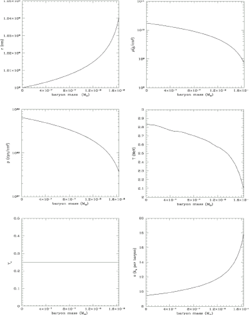
Since the wind is expected to be blown from a nearly hydrostatic PNS surface, the initial density profile of matter is determined by solving the Oppenheimer-Volkoff equation in this surface layer by setting the density at the innermost mesh as g/cm3 and assuming a constant value for the temperature and the electron fraction in the whole layer. In the present study, we take MeV and . By setting the matter pressure at the outer boundary (see equation (25)) by hand, there is a little deviation from a perfectly static configuration. We run the code for a short time without heating and cooling processes of neutrinos until a complete hydrostatic state is obtained for the given outer boundary condition. We adopt the resulting configuration as the initial condition. The hydrostatic distributions obtained by this procedure are shown in figure 1. The electron fraction remains constant (=0.25) because no neutrino reactions are included.
We have assumed a homogenous configuration for the initial magnetic fields. Thus, even after adding them to the matter distribution obtained above, the initial condition remains hydrostatic. As mentioned previously, the direction of the magnetic field is assumed to be perpendicular to the radial direction (, ). We adopt a magnetic field strength ranging from G (typical value for an ordinary NS) to G (suitable for a magnetar). Together with the non-magnetic model (model N), the models in this study are listed in Table 1. The names of these models are characterized by their initial plasma beta at the outer boundary.
| Model | (G) | (dyn/cm2) | ||
|---|---|---|---|---|
| N | 0 | 1.01022 | ||
| 106M | 1.01012 | 1.6106 | 1.0105 | 1.01022 |
| 103M | 1.01013 | 1.6104 | 1.0103 | 1.01022 |
| 10M | 1.01014 | 1.6102 | 1.010 | 1.01022 |
| 1M | 3.21014 | 1.610 | 1.0 | 9.91022 |
| M | 1.01015 | 1.6 | 1.010-1 | 9.01021 |
| M | 1.41015 | 7.910-1 | 5.010-2 | 8.01021 |
| M | 2.21015 | 3.210-1 | 2.010-2 | 6.31021 |
| M | 3.21015 | 1.610-1 | 1.010-2 | 4.71021 |
| M | 4.51015 | 7.910-2 | 5.010-3 | 2.61021 |
We have employed free inner and outer boundary conditions except for radius and velocity. At the inner boundary, the velocity is set to be zero, and radius is fixed in time.
Magnetic fields are defined at the mesh interfaces in the numerical code. Their inner boundary condition is given as
| (22) |
where the subscript I represents the innermost mesh interface. The outer boundary condition for magnetic fields is given as
| (23) |
where the subscript N stands for the outermost interface, and is the linear extrapolation of magnetic field given as
| (24) |
The third condition in equation (23) is imposed to avoid the negative magnetic field, although this situation has not occurred in our calculations. The outer boundary condition for the matter pressure is expressed in a similar way as
| (25) |
where is the linear extrapolation of matter pressure multiplied by a reduction factor 0.94, and is given as
| (26) |
The subscripts n and N denote, respectively, the outermost mesh center and interface. is constant which varies among the models (see Table 1). These values are chosen so as to give an asymptotic temperature suitable for r-process (MeV) in the final phase of the wind evolution. In fact, we have set to give the identical total pressure (dyn/cm2) at s. In order to suppress oscillations at the boundary, we have limited the boundary pressures to give only negative gradients. The extrapolation has been employed instead unlike the previous study of Ref. [8] so as to avoid an unrealistic accelerations at the outermost mesh point by the strong magnetic field (), which may produce a shock wave. The factor 0.94 which appears in equation (26) was employed only just it minimized the deviation from the hydrostatic state when making initial conditions, and there are no physical backgrounds. It is noted that the prescription has little influence on the overall dynamics.
3 Numerical results
We have computed all the models in Table 1 by the same procedure given in §2. The only difference in each model is the magnetic field strength and the value of , the boundary value of matter pressure. First, we show the numerical result of the non-magnetic wind case which was already studied by Ref. [8] (with a little change in the boundary conditions and numerical treatments of the basic equations). We have done this to check for the validity of our numerical method and to use the result for comparison with the magnetic wind solutions.
Figures 2-3 show the evolution of the non-magnetic model (model N). The r-process in the neutrino-driven wind proceeds as follows. At the surface of the PNS, matter is initially composed of relativistic particles, free nucleons, and photons. The nascent PNS contracts and releases ergs of gravitational energy mostly through neutrino production and emission over its Kelvin-Helmholtz cooling time (seconds), and a small fraction of the energy is deposited at the surface layer via following reactions.
| (27) |
| (28) |
| (29) |
| (30) |
| (31) |
| (32) |
| (33) |
Here the subscript denotes the flavor of neutrino (). Most efficient reactions to deposit energy are the neutrino absorption on free nucleons ((27) and (28)). These reactions also determine the evolution of the electron fraction. When sufficient energy is deposited to overcome the gravitational attraction, an outflow (neutrino-driven wind) is generated. The wind is heated until it reaches 50km. As the wind expands, the temperature decreases and when it drops below MeV, the free nucleons start to combine with each other and form -particles. At this stage, neutrino reactions have ceased, and the subsequent evolution becomes adiabatic. When the temperature drops below MeV, -process occurs (e.g. triple reactions), and seed nuclei of the r-process are formed until the temperature drops to MeV.
There are three key quantities in the wind scenario which determine the neutron-to-seed ratio. Those are the electron fraction () and entropy per baryon (), and the dynamical time scale (). The dynamical timescale is defined to be the duration of the -process. For a robust r-process, lower values are favored for and because it implies that neutrons are rich and the duration of the production of seed nuclei is short. Higher entropy is favored for the following reason. When the system is still in high temperature regime (above MeV), and nuclear statistical equilibrium (NSE) is maintained, the high entropy shifts the equilibrium to the state in which matter is composed mainly of particles and free neutrons with only a small fraction of nuclei. However, when the temperature becomes MeV, the system falls out of NSE. The high entropy implies a low density. Therefore, the -process proceeds slowly, and most of the matter remains as -particles.
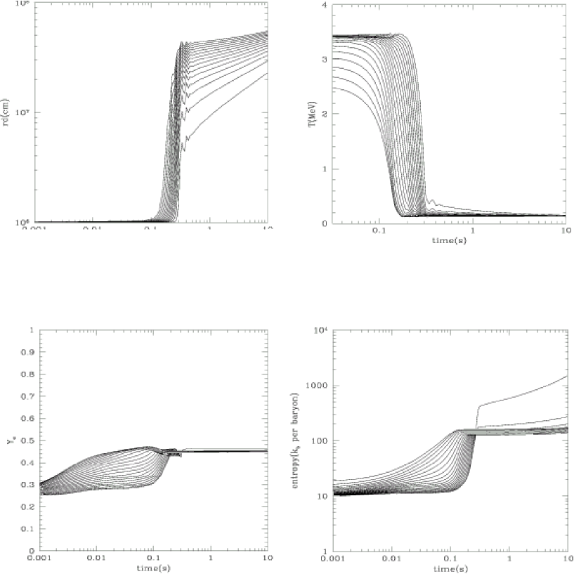
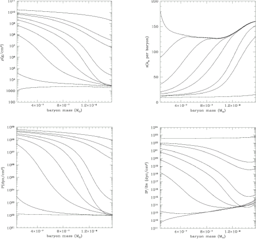
In model N, the wind expands rapidly 0.1 s after the beginning of neutrino heating processes. As the temperature decreases, the -processes occur, which corresponds to the location from 50km to 150km. The state is reached to the asymptotic one with a constant temperature 0.1MeV at 0.2s. Rapid increases of the electron fraction and entropy are seen when the wind is expanding from the surface of the PNS to 50km. Note that a slight increase of entropy in the late phase of the wind evolution is caused by a breakdown of approximation for the heating by electron and positron scatterings. This occurs because the equation we have used for the heating due to electron and positron scatterings is valid only when the temperature is high and, therefore, overestimates the increase of the entropy in the low temperature regime (see Ref. [8] for detail). This takes place in all the models commonly. However, this affects little the dynamics of the wind in this phase, and does not make a significant change in the dynamical time scale, electron fraction and entropy before the -process stage. Thus, we can safely discuss the possibility of r-process by ignoring this false increase in entropy. Figure 3 shows the baryon mass density , matter pressure , and entropy per baryon as a function of baryon mass. The density and pressure show significant decrease when the wind is expanding rapidly. Then the asymptotic state appears where g/cm3 and dyn/cm2 in the whole region. These features are identical with the previous studies done by Ref. [8]
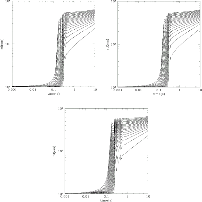
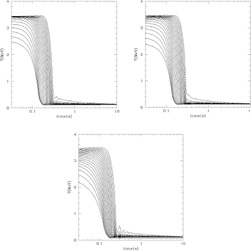
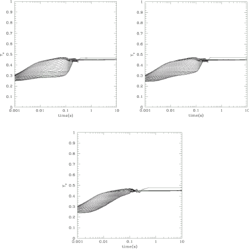
The trajectories of models M, M, and M are shown in figure 4. As the initial magnetic field becomes greater, more rapid expansion can be seen. However, the later evolution shows only little deviation from model N (see figure 7), and the overall evolution for all models is nearly identical with that for the non-magnetic model. Figures 5 and 6 present, respectively, the evolutions of temperature and electron fraction for models M, M, and M. As in model N, the efficient decrease in temperature and increase in electron fraction take place when the matter is rapidly expanding. The values of temperatures and electron fractions at the same radius almost coincide among all the models including model N. This implies that the models with stronger magnetic fields show an earlier drop in temperature and rise in the electron fraction, and the later behavior becomes identical. The asymptotic values of and do not vary so much among all models (0.45, MeV).
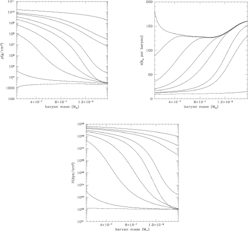
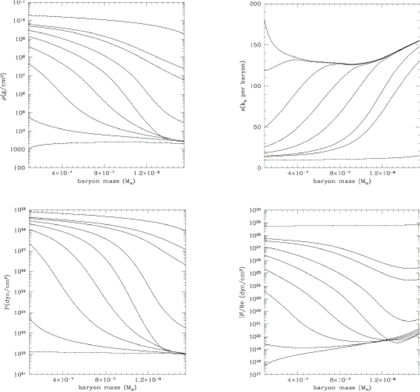
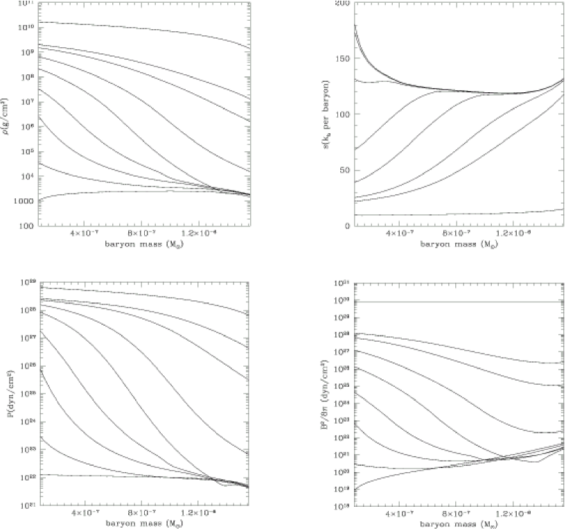
The distributions of the baryon mass density , entropy per baryon , matter pressure as well as magnetic pressure for these three models are given (as a function of the baryon mass) in figures 8-10. The evolutions of baryon mass density and pressure are essentially same in all models (including model N). The density and pressure decrease as the wind expands and reach an asymptotic value, which is nearly identical among all models (g/cm3, dyn/cm2). The evolutions of the magnetic pressure and entropy are also similar among the models except for the asymptotic value. As the wind expands, the initially homogeneous magnetic pressure decreases and reaches an asymptotic value. Unlike the density and pressure, the asymptotic value varies largely in the region. The final distribution of magnetic pressure has a positive gradient, and the outer region is 2 orders of magnitude larger than the inner region. Since the neutrino heating processes occur up to 50km, the entropy increases until the wind reaches that radius. The models with initially strong magnetic fields tend to have lower asymptotic values compared to the models with weaker fields. This tendency can be observed particularly in the outer region of the wind. As mentioned above, the more rapid evolutions of these values (, , , and ) seen in the models with stronger magnetic fields are results of the more rapid expansion. These behaviors will be discussed in more detail in the next section.
The three key quantities (, , and ) for the r-process are summarized for all the models in Table 2. Since the outer and inner regions are affected by the boundary conditions, the average values shown in the table are obtained by discarding the inner and outer 5 mesh points. The entropy in the table is the average value at the beginning of the -process (T0.5MeV). The false increase of entropy caused by the breakdown of the approximation in the late phase is ignored. The dynamical time scale is calculated as the duration, in which the temperature decreases from 0.5MeV to 0.2MeV, for each trajectory and averaged. As noted above, we can not see any significant difference in the trajectories of the magnetic wind cases and non-magnetic wind case. Even in the models with magnetar-scale field strengths, only a slight change comes out (the trajectories of model M together with model N are displayed in figure 7). Therefore, it is no surprise that the evolution of the variables such as temperature, electron fraction, density, pressure and entropy are also nearly identical (see figures 2-3 and 5-10). As a result, even strong magnetic fields give remarkably little change in the three key parameters (see Table 2). We will discuss the reason for this in the next section in greater detail.
| Model | |||
|---|---|---|---|
| N | 137 | 4.6310-2 | 0.453 |
| 106M | 137 | 4.5710-2 | 0.453 |
| 103M | 136 | 4.5710-2 | 0.453 |
| 10M | 136 | 4.5510-2 | 0.453 |
| 1M | 137 | 4.5510-2 | 0.453 |
| M | 136 | 4.4110-2 | 0.453 |
| M | 135 | 5.2710-2 | 0.453 |
| M | 133 | 5.3510-2 | 0.453 |
| M | 129 | 4.0110-2 | 0.453 |
| M | 128 | 5.4510-2 | 0.453 |
4 Discussions
Our results show that the homogenous magnetic field has only a little effect on the wind dynamics. In particular, the three key quantities for the r-process do not vary much from those for the non-magnetic wind. This is true even for the very strong magnetic fields. In this section, we will analyze this behavior in more detail.
The reason why the dynamics is little affected by magnetic fields is understood from the evolutions of magnetic fields. Figures 12-12 show the evolutions of the plasma beta, which is defined to be the ratio of matter pressure to magnetic pressure, for models M and M. In these models, the plasma beta increases rapidly from the initial values and the magnetic pressure becomes negligible for the wind dynamics. This tendency can be explained analytically as follows.
From equation (8), the variation rate of the magnetic pressure is given as
| (34) |
where denotes the Lagrange derivative, and is a radial fluid velocity which is defined as
| (35) |
Ignoring the neutrino heating, which is important only at the earliest stage, we can evaluate the variation rate of matter pressure approximately as
| (36) |
| (37) |
where is the adiabatic index. Ignoring further general relativistic corrections, can be approximated as
| (38) |
From the above equation, is written as
| (39) |
With the use of the continuity equation and equation (39), equations (34) and (36) become, respectively
| (40) |
| (41) |
If we locally approximate the velocity profile by a power-law, , the variation rates are evaluated as
| (42) |
| (43) |
Since the adiabatic index is approximately 4/3, we finally obtain the criterion that if , the plasma beta is decreased.
Figure 13 shows the radial profile of velocity for model N when the wind has settled to a quasi-steady state. Though this is a snapshot for this model, all the models have a similar configuration. If we apply the above criterion in this figure, we find that the region in which the plasma beta should decrease is the outer region (km). It is noted that the assumptions we have made to derive the above condition, that is, the adiabaticity and nonrelativisity of the flows, are clearly satisfied in the region. Thus, after the wind expands beyond 60km, the plasma beta will decrease. Since we are considering the region exterior to the PNS surface, the Newtonian gravity is not so bad an approximation in all region, and equation (42) is valid even in the inner region (km). On the other hand, equation (43) is not appropriate in this inner region, since the heating cannot be ignored and the adiabatic condition is not satisfied. However, it is obvious that the heating processes tend to increase the matter pressure and, as a result, increase the plasma beta more than in the adiabatic flow. Thus, although the obtained criterion is not valid, the plasma beta is expected to increase in the inner region where .
From the above discussions, the wind is expected to expand initially with increasing plasma beta up to 60km, and thereafter with decreasing plasma beta. Our numerical results actually agree with the expectation. This can be confirmed by seeing figures 12-12. Since the increase of the plasma beta occurs more rapidly than the following decrease, the wind tends to be matter-pressure-dominant in the entire evolution. Thus, even models with very strong magnetic fields give only a little effect on the wind evolution. In the following, we will further analyze, although small, effects of magnetic fields on the dynamics, focusing on model M.
At the beginning of expansion, the magnetic pressure is dominant, as can be seen from figures 8-10, and its negative gradient pushes the matter outward. This causes an early rapid expansion seen in figure 7. Although the magnetic pressure accelerates matter for a while, the effects of the magnetic pressure soon becomes significantly small (since the plasma beta decreases rapidly). Then, as they approach the asymptotic state, the gradient of the magnetic field changes signs and starts to decelerate matter (see figures 12-12). Note that although magnetic pressure is small at this stage, it still has some leverage on the dynamics to cancel the initial accelerations. This causes the later catch-up of non-magnetic wind model N seen in figure 7.
The subsequent distribution of the magnetic pressure is a direct consequence of the initial assumption on the magnetic field. The initial homogeneity of magnetic fields implies that the matter near the surface has a greater magnetic flux per unit mass compared with the matter deeper inside, since the density is higher there. As the wind evolves to an asymptotic state with a constant density in radius, the frozen-in magnetic field has a larger magnetic flux densities in the outer region. In another word, the final magnetic field configuration has an inverted profile of the initial matter density distribution.
This can be understood more precisely from equation (8) and figure 1. By using the same approximation that we have made previously, we can approximate equation (8) as
| (44) |
for arbitrary and . Taking and , respectively, as the initial time and the time at which the asymptotic state is reached, we find that , , and depend on very weakly. is also identical on all mesh points. Thus, the ratio of magnetic pressures between two mesh points in the asymptotic state can be approximated as
| (45) |
From the initial density distribution shown in figure 1 and the evolutions of density and magnetic pressure shown in figures 8-10, this relation is verified.
As a result of
the initial expansion and the later deceleration of the flow
mentioned above,
the key quantities for the r-process except for the electron fraction
show only a little change among the models. On the other hand, this
change depends on the initial location of mass element
in the atmosphere, which can be roughly divided into
(i) the outer region, (ii) the central region and
(iii) the inner region as follows:
(i) The outer region ()
Since the outer region has the lowest plasma beta,
the early rapid expansion occurs most
efficiently. Consequently, as matter passes
through the heating region rapidly, the resulting entropy becomes lower
compared with the non-magnetic wind. This effect can be seen by
comparing figure 3 with figures 8-10.
Moreover, the deceleration takes place
earlier on in the outer regions because the
density gradient is initially
larger than the inner regions.
This occurs during the -process stage, and makes the
dynamical time scale longer.
(ii) The central region ()
Though their plasma beta is not so low as in the outer region, the
initial rapid
expansion takes place also in this region and the entropy becomes
lower than for the non-magnetic wind.
Unlike the outer region, however, the deceleration occurs much later after the
wind has already passed through the -process region (50km
to 150km). Thus, the dynamical time scale becomes shorter.
The three key quantities in the central region are displayed for all
the models in Table 3, in which
we have taken average by excluding the outer
and inner 25 mesh points.
The reduction of the dynamical time scale in the models with strong magnetic
fields can be observed in the table. However,
the reduction is very small and, moreover, the
entropy decreases at the same time. Thus,
even if we focus only on this
region, a successful r-process will not take place.
| Model | |||
|---|---|---|---|
| N | 130 | 3.3710-2 | 0.453 |
| 106M | 130 | 3.3710-2 | 0.453 |
| 103M | 130 | 3.3710-2 | 0.453 |
| 10M | 130 | 3.3710-2 | 0.453 |
| 1M | 130 | 3.3510-2 | 0.453 |
| M | 129 | 3.3610-2 | 0.453 |
| M | 129 | 3.3310-2 | 0.453 |
| M | 133 | 3.0810-2 | 0.453 |
| M | 124 | 2.8310-2 | 0.453 |
| M | 121 | 2.7810-2 | 0.453 |
(iii) The inner region ()
The inner region also experiences the acceleration and
deceleration stages. However, because of their large initial plasma
beta, their effects are too small and
the key quantities for the r-process are essentially unaffected.
As mentioned previously in §2, our calculations approximate the flow near the equator with initial magnetic fields perpendicular to the radial direction. Our results can be applied to the places in the wind where the deviation from the radial motion is small, that is, regions where the radial force dominates over the transverse force. The angular range that satisfies this condition can be estimated as follows. For an arbitrary initial field-configuration, if the transverse velocity is small compared with the radial velocity, the magnetic fields are approximately determined by equations (7)-(9). In the nonrelativistic limit, these equations become
| (46) |
| (47) |
| (48) |
The evolution of the magnetic fields is determined by the initial magnetic fields, radius, and density, as well as by the present radius and density. The typical values for the initial radius and density, and the final radius and density in our models are 10km, 1010gcm-3, 500km, and 2103gcm-3, respectively. If the initial magnetic field is uniform and perpendicular to the the equatorial plane, the radial force dominates over the transverse force roughly in the angular range between . This occupies a significant fraction of the total solid angle, and our results are applicable to a rather large region below and above the equatorial plane.
5 Summary
In this paper we have investigated the effects of magnetic fields on the neutrino-driven wind and explored the possibility as an r-process site by performing numerical simulations. The homogenous distribution is assumed for the initial magnetic fields, and ten models with a wide range of field-strength have been computed.
The results do not give the dynamical behavior expected by Ref. [10] This may be the consequence of the assumed wind configuration, which has a tendency to increase the plasma beta rapidly and the matter-pressure is dominated in most of the wind evolutions. Hence, the magnetic pressure has little chance to influence the dynamics.
The evolutions of weak magnetic field models are identical with non-magnetic model. The models with very strong magnetic fields (G) show some, though not large, variation. For about of wind, the reduction of the dynamical time scale has been found. However, this change is very small and accompanied by the decreases of entropy. Thus, unfortunately, the situation favored for a successful r-process is not realized in our models, even with magnetar-scale field-strengths.
Since our study has been limited to initially homogeneous magnetic fields, other distributions of magnetic field should be investigated. Note, however, that the initial surface structure will be changed substantially then, since the magnetic pressure will determine the hydrostatic force balance. Multi-dimensional MHD simulations of magnetar formation may shed a light on this issue. It is also self-evident that more realistic and multidimensional investigations will be needed further, since the field-tension that is not considered in this paper may play an important role. Even in that case, very strong magnetic fields G will be needed to influence the wind dynamics. Last but not least, magnetic reconnections might be interesting, since the dissipation of magnetic fields will heat the matter, accelerating the wind. However, this is much beyond the scope of this paper.
Acknowledgements
Some of the numerical simulations were done on the supercomputer VPP700E/128 at RIKEN and VPP500/80 at KEK (KEK Supercomputer Projects No.108). This work was partially supported by the Grants-in-Aid for the Scientific Research (14740166, 14079202) from Ministry of Education, Science and Culture of Japan and by Grants-in-Aid for the 21th century COE program “Holistic Research and Education Center for Physics of Self-organizing Systems”.
References
- [1] S. E. Woosley, J. R. Wilson, G. J. Mathews, R. D. Hoffman and B. S. Meyer, \AJ433,1994,229
- [2] J. Witti, H. -Th. Janka and Takahashi, A&A 286 (1994), 841
- [3] K. Takahashi, J. Witti and H. -Th. Janka, A&A 286 (1994), 857
- [4] Y. -Z. Qian and S. E. Woosley, \AJ471,1996,331
- [5] C. Y. Cardall and G. M. Fuller, \AJ486,1997,111
- [6] K. Otsuki, H. Tagoshi, T. Kajino and S. Wanajo, \AJ533,2000,10
- [7] S. Wanajo, T. Kajino, G. J. Mathews and K. Otsuki, \AJ554,2001,578
- [8] K. Sumiyoshi, H. Suzuki, K. Otsuki, M. Terasawa and S.Yamada, PASJ 52 (2000), 601
- [9] S. Nagataki and K.Kohri, PASJ 53 (2001), 547
- [10] T. A. Thompson, \AJ585,2003,33
- [11] S. Yamada, \AJ475,1997,720
- [12] C. W. Misner and D. H .Sharp, \PRB136,1964,571
- [13] A. Achterberg, \PRA28,1983,2449
- [14] H. Shen, H. Toki, K. Oyamatsu and K. Sumiyoshi, \NPA637,1998,435
- [15] H. Shen, H. Toki, K. Oyamatsu and K. Sumiyoshi, \PTP100,1998,1013
- [16] Y. -Z. Qian, Prog. Part. Nucl. Phys. 50 (2003),153
- [17] R. D. Hoffman, S. E. Woosley and Y. -Z. Qian, \AJ482,1997,951
- [18] M. Terasawa, K. Sumiyoshi, S. Yamada, H. Suzuki and T. Kajino, \AJ578,2002,137
- [19] C. Sneden, A. McWilliam, G. W. Preston and J. J. Cowan, \AJ467,1996,819
- [20] Y. Ishimaru and S. Wanajo, \AJ511,1999,33
- [21] T. Tsujimoto, T. Shigeyama and Y. Yoshii, \AJ519,1999,63
- [22] S. Wanajo, N. Itoh, Y. Ishimaru, S. Nozawa and T. C. Beers, \AJ577,2002,853
- [23] D. Argast, M. Samland, F. -K. Thielemann and Y. -Z. Qian, A&A 416 (2004), 997