A relativistic model of the radio jets in NGC 315

Abstract

We apply our intrinsically symmetrical, decelerating relativistic jet model to deep VLA imaging of the inner $\pm$70 arcsec of the giant low-luminosity radio galaxy NGC 315. An optimized model accurately fits the data in both total intensity and linear polarization. We infer that the velocity, emissivity and field structure in NGC 315 are very similar to those of the other low-luminosity sources we have modelled, but that all of the physical scales are larger by a factor of about 5. We derive an inclination to the line of sight of $38^{\circ}\pm 2^{\circ}$ for the jets. Where they first brighten, their on-axis velocity is $\beta=v/c\approx 0.9$. They decelerate to $\beta\approx 0.4$ between 8 and 18 kpc from the nucleus and the velocity thereafter remains constant. The speed at the edge of the jet is $\approx$0.6 of the on-axis value where it is best constrained, but the transverse velocity profile may deviate systematically from the Gaussian form we assume. The proper emissivity profile is split into three power-law regions separated by shorter transition zones. In the first of these, at $\approx$3 kpc (the flaring point) the jets expand rapidly at constant emissivity, leading to a large increase in the observed brightness on the approaching side. At $\approx$10 kpc, the emissivity drops abruptly by a factor of 2. Where the jets are well resolved their rest-frame emission is centre-brightened. The magnetic field is modelled as random on small scales but anisotropic and we rule out a globally ordered helical configuration. To a first approximation, the field evolves from a mixture of longitudinal and toroidal components to predominantly toroidal, but it also shows variations in structure along and across the jets, with a significant radial component in places. Simple adiabatic models fail to fit the emissivity variations.

1 Introduction

It was first recognised by Fanaroff & Riley (1974) that the ways in which extragalactic jets dissipate energy to produce observable radiation differ for high- and low-luminosity sources. Jets in low-luminosity (FR I) sources are bright close to the nucleus of the parent galaxy, whereas those in powerful (FR II) sources are relatively faint until their terminal hot-spots. It rapidly became accepted that FR I jets must decelerate by entrainment of the surrounding IGM (Baan, 1980; Begelman, 1982; Bicknell, 1984, 1986; De Young, 1996, 2004; Rosen et al., 1999; Rosen & Hardee, 2000) or by injection of mass lost by stars within the jet volume (Phinney, 1983; Komissarov, 1994; Bowman, Leahy & Komissarov, 1996).

More recently, evidence has accumulated that FR I jets are initially relativistic and decelerate on kpc scales. FR I sources are thought to be the side-on counterparts of BL Lac objects, in which relativistic motion on parsec scales is well-established (Urry & Padovani, 1995). Proper motions corresponding to speeds comparable with and in some cases exceeding $c$ have been measured on milliarcsecond scales in several FR I jets (Giovannini et al., 2001) and on arcsecond scales in M 87 and Cen A (Biretta, Zhou & Owen, 1995; Hardcastle et al., 2003). In FR I sources (as in FR IIs), the lobe containing the main (brighter) jet is less depolarized than the counter-jet lobe (Morganti et al., 1997). This can be explained as an effect of Faraday rotation in the surrounding halo of hot plasma if the main jet points toward the observer, suggesting that the brightness asymmetry is caused by Doppler beaming (Laing, 1988). The decrease of this asymmetry with distance from the nucleus (Laing et al., 1999) indicates deceleration.

The present paper is the third in a series devoted to modelling the jets in FR I radio galaxies. We assume that the jets are intrinsically symmetrical, axisymmetric, relativistic flows and we parameterize their geometry and the three-dimensional variations of their velocity, emissivity and magnetic-field structure. We then compute the brightness distributions in total intensity and linear polarization. By fitting simultaneously to deep, high-resolution radio images in Stokes $I$, $Q$ and $U$, we can optimize the model parameters. The fits are empirical, and make as few assumptions as possible about the (poorly-known) internal physics of the jets. The technique was originally developed to model the radio galaxy 3C 31 by Laing & Bridle (2002a, hereafter LB) and was then slightly revised and applied to B2 0326+39 and B2 1553+24 by Canvin & Laing (2004, hereafter CL). We now present a model for the jets in the well-known nearby radio galaxy NGC 315. This source has a huge angular and physical size (Bridle et al., 1976) and, as we shall show, the angular scales on which flaring, recollimation and deceleration of the jets take place are much larger than in the sources we have studied so far. Our results for NGC 315 therefore give a more detailed picture of the initial propagation of an FR I jet.

In order to improve on our empirical models, we need to understand the energy gain and loss processes affecting the ultrarelativistic particles which produce the observed synchrotron radiation. A self-consistent, axisymmetric adiabatic model fails to fit either the total intensity or the polarization distributions in the jets of 3C 31 within 5 kpc of the nucleus (Laing & Bridle, 2004). This suggests that injection of relativistic particles and/or amplification of the magnetic field are required, which is not surprising in view of the detection of cospatial X-ray synchrotron emission (Hardcastle et al., 2002). Further out in 3C 31, the adiabatic model gives a tolerable fit. A simple, quasi-one-dimensional analysis (LB, CL) is adequate to assess whether fitting of more elaborate models is worthwhile, and we apply this to NGC 315.

Given a kinematic model for the jets and estimates of the external density and pressure from X-ray observations, we can apply conservation of mass, momentum and energy to deduce the variations of internal pressure, density, Mach number and entrainment rate with distance from the nucleus (Laing & Bridle, 2002b).

In Section 2, we introduce NGC 315 and briefly summarize the VLA observations. Our modelling technique is outlined in Section 3, emphasizing the (small) differences from the earlier work of CL. The observed and model brightness distributions are compared in Section 4 and the derived geometry, velocity, emissivity and field distributions are presented in Section 5. We summarize our conclusions and outline our future programme in Section 6.

We adopt a concordance cosmology with Hubble constant, $H_{0}$ = 70 $\rm{km\,s^{-1}\,Mpc^{-1}}$, $\Omega_{\Lambda}=0.7$ and $\Omega_{M}=0.3$, although only the choice of $H_{0}$ is significant at the distance of NGC 315.

2 Observations and images

2.1 NGC 315

Our modelling technique requires that both radio jets are:

1. detectable with good signal-to-noise ratio in total intensity and linear polarization;

2. straight and antiparallel;

3. separable from any surrounding lobe emission and

4. asymmetric, in the sense that their jet/counter-jet intensity ratio is significantly larger than unity over a significant area.

The nearby giant elliptical galaxy NGC 315, whose large-scale radio structure was first imaged by Bridle et al. (1976), is one of the brightest sources satisfying these criteria. The galaxy has a redshift of 0.01648 (Trager et al., 2000), giving a scale of 0.335 kpc arcsec^-1 for our adopted cosmology. The overall extent of the radio source is approximately 3500 arcsec, or about 1200 kpc in projection, but the area to be modelled (see Fig. 1) is limited in extent by the slight bends in the jet at roughly 70 arcsec (23 kpc in projection) from the nucleus (see Section 3.2).

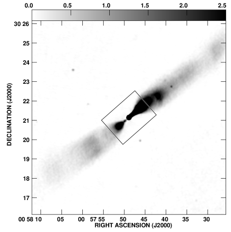
Figure 1: A grey-scale of the large-scale structure of the jets in NGC 315 at a resolution of 5.5 arcsec FWHM. The image is the mean of four at different frequencies between 1.365 and 1.665 GHz and is described in Laing et al. (in preparation). The grey-scale range is 0 – 2.5 mJy (beam area)^-1 as shown by the labelled wedge and the modelled area is indicated by the box.

High-resolution images of the jets on kpc scales were presented by Bridle et al. (1979), Fomalont et al. (1980) and Venturi et al. (1993) and on pc scales by Linfield (1981), Venturi et al. (1993), Cotton et al. (1999) and Xu et al. (2000). More comprehensive references to radio, optical and X-ray observations of NGC 315 are given by Laing et al. (in preparation).

2.2 Observations and data reduction

The observations and their reduction are also described in detail by Laing et al. (in preparation). We fit to images made using the 5 GHz dataset from that paper at 2.35 and 0.40 arcsec FWHM [the higher-resolution images are also discussed and compared with Chandra observations by Worrall et al. (in preparation)]. The dataset includes long observations in all four configurations of the VLA and provides excellent sampling of spatial scales between 0.4 and 300 arcsec. The resolutions and noise levels are given in Table 1.

Table 1: Image resolutions and noise levels. $\sigma_{I}$ is the off-source noise level on the $I$ image; $\sigma_{P}$ the average of the noise levels for $Q$ and $U$.

FWHM	rms noise level
(arcsec)	[$\mu$Jy (beam area)-1]
	$\sigma_{I}$	$\sigma_{P}$
2.35	10.0	7.5
0.40	12.5	6.8

The accuracy of linear polarization measurements is critical to our technique. The E-vector position angles have been corrected to zero wavelength using an image of rotation measure derived from 5-frequency observations at a resolution of 5.5 arcsec FWHM between 1.365 and 5 GHz (Laing et al., in preparation). Significant corrections are required for the mean Faraday rotation ($-76$ rad m^-2) and a linear gradient along the jet, both probably of Galactic origin. The fitting errors are typically $\la$2.5 rad m^-2 in the area of interest, corresponding to position angle rotation $\la$0.5^∘ at 5 GHz. The observed fluctuations of rotation measure on scales of a few beamwidths are very small ($\approx$1 – 2 rad m^-2) and residual depolarization is undetectable, so errors in E-vector position angle and degree of polarization $p=(Q^{2}+U^{2})^{1/2}/I$ due to changes in Faraday rotation across the 5.5 arcsec beam should be negligible. Observations at two centre frequencies (4.860 and 4.985 GHz) were combined to make the final dataset (Laing et al., in preparation) but the error in E-vector position angle due to this effect is $<$1^∘. Depolarization due to rotation across the maximum bandwidth of 50 MHz is also negligible. The modelling described later is not affected by Ricean bias (Wardle & Kronberg, 1974), as we fit to Stokes $I$, $Q$ and $U$ directly, but our plots of the degree of polarization include a first-order correction for this effect. We plot the direction of the apparent magnetic field, rotated from the zero-wavelength E-vector position angles by 90^∘.

3 The model

3.1 Assumptions

Our fundamental assumptions are those of LB and CL:

1. The jets may be modelled as intrinsically symmetrical, antiparallel, axisymmetric, stationary, laminar flows. The real flow is clearly much more complicated, but all that is necessary for our technique to work is that an average over a sufficiently large volume results in statistically identical rest-frame emission from the main and counter-jets. In poorly resolved cases, some care is required to distinguish between intrinsic variations of physical parameters and local fluctuations such as knots and filaments, as we will discuss.

2. The jets contain relativistic particles with an energy spectrum $n(E)dE=n_{0}E^{-(2\alpha+1)}dE$ (corresponding to a frequency spectral index $\alpha$) with an isotropic pitch-angle distribution. The maximum degree of linear polarization is then $p_{0}=(3\alpha+3)/(3\alpha+5)$. We use $\alpha=0.55$, the mean spectral index for the modelled region between 1.365 and 5 GHz (Laing et al., in preparation).

3. The magnetic field is tangled on small scales, but anisotropic (the reasons for taking the field to be of this form are discussed by Laing 1981, Begelman et al. 1984 and LB; see also Section 5.5).

4. The emission is optically thin everywhere. The core, which is unresolved in our VLA observations and partially optically thick, is not modelled. It is represented as a point source with the correct flux density.

We define $\beta=v/c$, where $v$ is the flow velocity. $\Gamma=(1-\beta^{2})^{-1/2}$ is the bulk Lorentz factor and $\theta$ is the angle between the jet axis and the line of sight.

3.2 Outline of the method

The jet/counter-jet intensity ratio for intrinsically symmetrical, relativistic jets depends on the product $\beta\cos\theta$, so the angle to the line of sight and velocity cannot be decoupled by observations of $I$ alone. The basis of our technique is that relativistic aberration causes the approaching and receding jets to appear different not only in total intensity, but also in linear polarization. We use these polarization differences as independent constraints in order to break the degeneracy between $\beta$ and $\theta$. An outline of our procedure is as follows.

1. Develop a parameterized description of the geometry, velocity, emissivity and magnetic-field ordering.

2. Calculate the synchrotron emission in $I$, $Q$ and $U$ from the model jets by numerical integration, taking account of relativistic aberration.

3. Convolve and compare with deep VLA images, using $\chi^{2}$ to measure the quality of the fit.

4. Optimize the model parameters using the downhill simplex method.

The details of the calculations are fully described by LB and CL.

The assumption of axisymmetry is clearly violated in NGC 315 at $\approx$70 arcsec from the nucleus. Both jets bend clockwise by $\approx$5^∘ (in projection) at this distance, but we do not know the magnitude of any associated bends in the orthogonal direction. Our modelling could be extended to larger distances provided that the jets are indeed antiparallel and intrinsically identical after the bends. This seems plausible from their appearance in projection and we could fit independently for the angle to the line of sight after the bend if necessary. The brightness and polarization structures of the jets are qualitatively consistent with an extrapolation of the fitted model described below, so it is likely that this approach would succeed. It adds significant complexity to the modelling procedure, however, and also requires careful justification of the assumption of intrinsic symmetry at large distances. For these reasons, we defer this analysis to a later paper.

3.3 Functional forms for geometry, velocity, magnetic field and emissivity

The functional forms used to parameterize the geometry, velocity, emissivity and magnetic field are very similar to those described by CL, which are in turn an evolution from those introduced by LB. The earlier papers discuss the motivation of these expressions in detail; here we just summarize their forms for completeness and to highlight a few differences from our earlier work.

3.3.1 Geometry

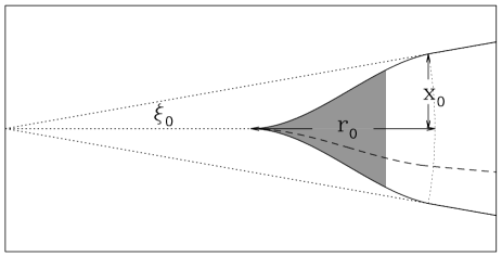
Figure 2: A sketch of the assumed jet geometry, defining the quantities $\xi_{0}$, $r_{0}$ and $x_{0}$ used in Table 3. For NGC 315, the modelled area (indicated schematically by shading) is entirely within the flaring region. The full line indicates the edge of the jet ($s=1$) and the dashed line the $s=0.5$ streamline.

The assumed geometry, sketched in Fig. 2 is derived from a fit to the outer isophote of the jet emission. It is identical to that used by CL, but in this case we model only the flaring region where the jet expands rapidly and then recollimates. NGC 315 also shows a conical outer region of constant (very small) opening angle, as seen in other FR I jets, but this is beyond the bends which limit our ability to fit an axisymmetric model directly to the observed data.

We define $z$ to be the distance from the nucleus along the axis and $\xi_{0}$ to be the half-opening angle of the jet in the outer region. As in CL, our assumed flow streamlines are a family of curves one of whose members is defined by the outer boundary of the jet. We use a streamline coordinate system $(\rho,s)$ where the streamline index $s$ is constant for a given streamline and $\rho$ increases monotonically with distance along it. In the outer region, the streamlines are assumed to be radial from a point on the axis with $z=-A$, where $A=x_{0}/\sin\xi_{0}-r_{0}$. For a streamline which makes an angle $\xi$ with the jet axis in the outer region, we define $s=\xi/\xi_{0}$, so $s=0$ on-axis and $s=1$ at the edge (Fig. 2). The distance of a streamline from the jet axis in the flaring region is:

$$x(z,s) = a_{2}(s)z^{2}+a_{3}(s)z^{3}$$

The curve is constrained to fit the jet boundary for $s=1$ and the coefficients are determined by the conditions that $x(s)$ and its first derivative are continuous at the boundary between the regions. $\rho$ is defined by:

$$\rho = \frac{zr_{0}}{(r_{0}+A)\cos(\xi_{0}s)-A}\hskip 28.45274pt\rho<r_{0}$$

and varies monotonically along a streamline from 0 at the nucleus to $r_{0}$ at the spherical surface defining the end of the flaring region.

3.3.2 Velocity

The form of the velocity field $\beta(\rho,s)$ is the same as that used by CL. The on-axis velocity profile is divided into three parts:

1. roughly constant, with a high velocity $\beta_{1}$, close to the nucleus;

2. a linear decrease and

3. roughly constant but with a low velocity $\beta_{0}$ at large distances.

[the velocities in (i) and (iii) are not quite constant because transitions between regions are smoothed to avoid numerical problems]. The profile is defined by four free parameters: the distances of the two boundaries separating the three regions, $\rho_{\rm v_{1}}$ and $\rho_{\rm v_{0}}$, and the characteristic inner and outer velocities $\beta_{1}$ and $\beta_{0}$. Off-axis, the velocity is calculated using the same expressions but with inner and outer velocities $\beta_{1}\exp(-s^{2}\ln v_{1})$ and $\beta_{0}\exp(-s^{2}\ln v_{0})$, i.e. with a truncated Gaussian transverse profile falling to fractional velocities $v_{1}$ and $v_{0}$ at the edge of the jet in the inner and outer regions, respectively.

The full functional forms for the velocity field $\beta(\rho,s)$ are given in Table 2.

3.3.3 Magnetic field

We define the rms components of the magnetic field to be $\langle B_{l}^{2}\rangle^{1/2}$ (longitudinal, parallel to a streamline), $\langle B_{r}^{2}\rangle^{1/2}$(radial, orthogonal to the streamline and outwards from the jet axis) and $\langle B_{t}^{2}\rangle^{1/2}$ (toroidal, orthogonal to the streamline in an azimuthal direction). The magnetic-field structure is parameterized by the ratio of rms radial/toroidal field, $j(\rho,s)=\langle B_{r}^{2}\rangle^{1/2}/\langle B_{t}^{2}\rangle^{1/2}$ and the longitudinal/toroidal ratio $k(\rho,s)=\langle B_{l}^{2}\rangle^{1/2}/\langle B_{t}^{2}\rangle^{1/2}$. The parameterization is similar to that used by CL, but we also allow variation of the field component ratios with $s$ (cf. LB) in order to improve the fit to the variation of polarization across the jets, which is better resolved in NGC 315 than in the sources modelled by CL. For each of the axial ($s=0$) and edge ($s=1$) streamlines, the field ratios have constant values for $\rho<\rho_{\rm B_{1}}$ and $\rho>\rho_{\rm B_{0}}$, with linear interpolation between them for $\rho_{\rm B_{1}}\leq\rho\leq\rho_{\rm B_{0}}$. For intermediate streamlines, we then interpolate linearly between the ratios for $s=0$ and $s=1$.

The functional forms assumed for the field ratios are again given in Table 2.

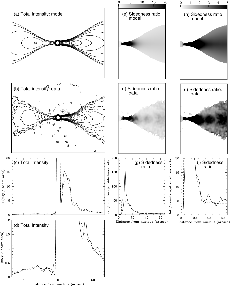
Figure 3: A comparison of the model and data in total intensity at 2.35 arcsec resolution for the inner 66.5 arcsec of each jet. (a) model contours; (b) observed contours. The contour levels in panels (a) and (b) are $-2$, $-1$, 1, 2, 4, 8, 12, 20, 36, 60, 100, 160, 250, 400, 600, 1000 $\times$ 30 $\mu$Jy (beam area)^-1. (c) and (d) $I$ profiles along the jet axis for the data (solid line) and model (dashed line). (e) and (f) Grey-scales of sidedness ratio, obtained by dividing total-intensity images by copies of themselves rotated by 180^∘ about the core. The ratio is in the sense main jet / counter-jet. (e) model; (f) data. (g) profile of sidedness ratio along the jet axis for the data (solid line) and model (dashed line). (h) – (j) as (e) – (g), but with smaller grey-scale and profile ranges to emphasise the variation of sidedness in the outer parts of the modelled region.

3.3.4 Emissivity

We write the proper emissivity as $\epsilon(\rho,s)h(\rho,s)$, where $\epsilon$ is the emissivity in $I$ for a magnetic field $B=\langle B_{l}^{2}+B_{r}^{2}+B_{t}^{2}\rangle^{1/2}$ perpendicular to the line of sight. $h$ depends on field geometry: for $I$, $0\leq h\leq 1$ and for $Q$ and $U$ $-p_{0}\leq h\leq+p_{0}$. We refer to $\epsilon$, loosely, as ‘the emissivity’. For a given spectral index, it is a function only of the rms total magnetic field and the normalizing constant of the particle energy distribution, $\epsilon\propto n_{0}B^{1+\alpha}$.

The on-axis emissivity profile consists of five regions, each with a power-law variation of $\epsilon$ with $\rho$. The profile for NGC 315 is consistent with a continuous variation of emissivity, so we enforce continuity everywhere ($g=1$ in the notation of CL). We use the expressions given by CL, but change the notation slightly in the interests of greater clarity. The profile is defined by five power-law indices and four boundary positions. As explained in more detail in Section 5.4, there are three primary emissivity regions with indices $E_{\rm in}$, $E_{\rm mid}$ and $E_{\rm out}$. The remaining two regions are introduced to model the transitions between them. The first (slope $E_{\rm rise}$) replaces the discontinuous increase in emissivity used to model the initial brightening of the jets in 3C 31 and B2 0326+39 (LB, CL) because the equivalent structure in NGC 315 is better resolved. The second (slope $E_{\rm fall}$), which models an abrupt decrease in emissivity, is equivalent to $E_{3}$ in the models of B2 0326+39 and B2 1553+24 (CL).

Off-axis, the profile is multiplied by a factor $\exp[-s^{2}\ln\bar{e}(\rho)]$, so that $\bar{e}(\rho)$ is the fractional value of the emissivity at the jet edge. $\bar{e}(\rho)$ has a constant value $e_{0}$ for $\rho>\rho_{\rm e_{3}}$ and varies linearly through regions 2 and 3 from $e_{1}$ at $\rho_{\rm e_{1}}$ to $e_{0}$ at $\rho_{\rm e_{3}}$. For $\rho<\rho_{\rm e_{1}}$, the jet is too narrow for our data to constrain any transverse profile and we set $\bar{e}(\rho)=1$.

The full description of the emissivity distribution $\epsilon(\rho,s)$ is given in Table 2.

Table 2: Functional forms of the velocity $\beta$, emissivity $\epsilon$, radial/toroidal and longitudinal/toroidal magnetic-field ratios $j$ and $k$ in the streamline coordinate system $(\rho,s)$. Column 4 lists the parameters which may be optimized, for comparison with Table 3.

Quantity	Functional form	Range	Free parameters
Velocity field
$\beta(\rho,s)$	$\beta_{1}-\left[\frac{\beta_{1}\exp(-s^{2}\ln v_{1})-\beta_{0}\exp(-s^{2}\ln v_{0})}{10}\right]\exp[c_{1}(\rho-\rho_{\rm v_{1}})]$	$\rho<\rho_{\rm v_{1}}$	Distances $\rho_{\rm v_{1}}$, $\rho_{\rm v_{0}}$
	$c_{2}+c_{3}\rho$	$\rho_{\rm v_{1}}\leq\rho\leq\rho_{\rm v_{0}}$	Velocities $\beta_{1}$, $\beta_{0}$
	$\beta_{0}+\left[\frac{\beta_{1}\exp(-s^{2}\ln v_{1})-\beta_{0}\exp(-s^{2}\ln v_{0})}{10}\right]\exp[c_{4}(\rho_{\rm v_{0}}-\rho)]$	$\rho>\rho_{\rm v_{0}}$	Fractional edge velocities $v_{1}$, $v_{0}$
Emissivity
$\epsilon(\rho,s)$	$~{}~{}~{}\left(\frac{\rho}{\rho_{\rm e_{1}}}\right)^{-E_{\rm in}}$	$\rho\leq\rho_{\rm e_{1}}$	Distances $\rho_{\rm e_{1}}$, $\rho_{\rm e_{2}}$, $\rho_{\rm e_{3}}$, $\rho_{\rm e_{4}}$
	$\left(\frac{\rho}{\rho_{\rm e_{1}}}\right)^{-E_{\rm rise}}\exp\left[-s^{2}\ln\left(e_{1}+(e_{0}-e_{1})\left(\frac{\rho-\rho_{\rm e_{1}}}{\rho_{\rm e_{2}}-\rho_{\rm e_{1}}}\right)\right)\right]$	$\rho_{\rm e_{1}}<\rho\leq\rho_{\rm e_{2}}$	Indices $E_{\rm in}$, $E_{\rm rise}$, $E_{\rm mid}$, $E_{\rm fall}$, $E_{\rm out}$
	$d_{1}\left(\frac{\rho}{\rho_{\rm e_{2}}}\right)^{-E_{\rm mid}}\exp\left[-s^{2}\ln\left(e_{1}+(e_{0}-e_{1})\left(\frac{\rho-\rho_{\rm e_{1}}}{\rho_{\rm e_{2}}-\rho_{\rm e_{1}}}\right)\right)\right]$	$\rho_{\rm e_{2}}<\rho\leq\rho_{\rm e_{3}}$	Fractional edge emissivities $e_{1}$, $e_{0}$
	$d_{2}\left(\frac{\rho}{\rho_{\rm e_{3}}}\right)^{-E_{\rm fall}}\exp(-s^{2}\ln e_{0})$	$\rho_{\rm e_{3}}<\rho\leq\rho_{\rm e_{4}}$
	$d_{3}\left(\frac{\rho}{\rho_{\rm e_{4}}}\right)^{-E_{\rm out}}\exp(-s^{2}\ln e_{0})$	$\rho>\rho_{\rm e_{4}}$
Radial/toroidal field ratio
$j(\rho,s)$	$j_{1}^{\rm axis}+s(j_{1}^{\rm edge}-j_{1}^{\rm axis})$	$\rho\leq\rho_{\rm B_{1}}$	Distances $\rho_{\rm B_{1}}$, $\rho_{\rm B_{0}}$
	$j^{\rm axis}+s(j^{\rm edge}-j^{\rm axis})$	$\rho_{\rm B_{1}}<\rho<\rho_{\rm B_{0}}$	Ratios $j_{1}^{\rm edge}$, $j_{0}^{\rm edge}$, $j_{1}^{\rm axis}$, $j_{0}^{\rm axis}$
	where  $j^{\rm axis}=j_{1}^{\rm axis}+(j_{0}^{\rm axis}-j_{1}^{\rm axis})\left(\frac{\rho-\rho_{\rm B_{1}}}{\rho_{\rm B_{0}}-\rho_{\rm B_{1}}}\right)$
	$j^{\rm edge}=j_{1}^{\rm edge}+(j_{0}^{\rm edge}-j_{1}^{\rm axis})\left(\frac{\rho-\rho_{\rm B_{1}}}{\rho_{\rm B_{0}}-\rho_{\rm B_{1}}}\right)$
	$j_{0}^{\rm axis}+s(j_{0}^{\rm edge}-j_{0}^{\rm axis})$	$\rho\geq\rho_{\rm B_{0}}$
Longitudinal/toroidal field ratio
$k(\rho,s)$	$k_{1}^{\rm axis}+s(k_{1}^{\rm edge}-k_{1}^{\rm axis})$	$\rho\leq\rho_{\rm B_{1}}$	Ratios $k_{1}^{\rm edge}$, $k_{0}^{\rm edge}$, $k_{1}^{\rm axis}$, $k_{0}^{\rm axis}$
	$k^{\rm axis}+s(k^{\rm edge}-k^{\rm axis})$	$\rho_{\rm B_{1}}<\rho<\rho_{\rm B_{0}}$
	where  $k^{\rm axis}=k_{1}^{\rm axis}+(k_{0}^{\rm axis}-k_{1}^{\rm axis})\left(\frac{\rho-\rho_{\rm B_{1}}}{\rho_{\rm B_{0}}-\rho_{\rm B_{1}}}\right)$
	$k^{\rm edge}=k_{1}^{\rm edge}+(k_{0}^{\rm edge}-k_{1}^{\rm edge})\left(\frac{\rho-\rho_{\rm B_{1}}}{\rho_{\rm B_{0}}-\rho_{\rm B_{1}}}\right)$
	$k_{0}^{\rm axis}+s(k_{0}^{\rm edge}-k_{0}^{\rm axis})$	$\rho\geq\rho_{\rm B_{0}}$

3.4 Fitting, model parameters and errors

The noise level for the calculation of $\chi^{2}$ for $I$ is estimated as $1/\sqrt{2}$ times the rms of the difference between the image and a copy of itself reflected across the jet axis. For linear polarization, the same level is used for both $Q$ and $U$. This is the mean of $1/\sqrt{2}$ times the rms of the difference image for $Q$ and the summed image for $U$, since the latter is antisymmetric under reflection for an axisymmetric model. This prescription is identical to that used by LB and CL. The region immediately around the core is excluded from the fit. $\chi^{2}$ is calculated using the high-resolution (0.4 arcsec) images where they have adequate signal-to-noise ratio (0.9 – 17 arcsec from the nucleus) and the lower-resolution (2.35 arcsec) images elsewhere (17 – 67 arcsec). The same fitting regions are used for total intensity and linear polarization and $\chi^{2}$ values for $I$, $Q$ and $U$ are summed over grids chosen so that all points are independent.

Figure 4: A comparison of the model and data in total intensity at 0.4 arcsec resolution for the inner 21 arcsec of the main jet. (a) model contours; (b) observed contours. The contour levels in panels (a) and (b) are $-2$, $-1$, 1, 2, 4, 8, 12, 20, 36, 60, 100, 160, 250, 400, 600, 1000 $\times$ 30 $\mu$Jy/beam area. (c) $I$ profile along the jet axis for the data (solid line) and model (dashed line).

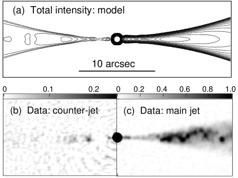
Figure 5: A comparison of the model and data in total intensity at 0.4 arcsec resolution for the inner $\pm$30 arcsec. (a) Model contours. The levels are logarithmic, increasing by factors of $\sqrt{2}$ from 4.24 – 543 $\mu$Jy (beam area)^-1. (b) Grey-scale of observed emission from the counter-jet. The range is 0 – 0.25 mJy (beam area)^-1. (c) as in panel (b), but for the main jet with a range of 0 – 1 mJy (beam area)^-1. This display emphasizes the fine-scale structure in both jets which cannot be described by the model, but shows that the gross features of the predicted and observed brightness distributions are very similar.

Figure 6: Average transverse profiles of total intensity at a resolution of 2.35 arcsec. The profiles are generated by averaging along radii between 45 and 66.5 arcsec from the nucleus and plotting against angle from the jet axis. The data are represented by the full line and the model by the dashed line. (a) main jet; (b) counter-jet. The jets are not perfectly straight, so there is a slight offset between the observed and model profiles over this range of distances.

Figure 7: Average transverse profiles of the jet/counter-jet sidedness ratio $I_{\rm j}/I_{\rm cj}$ at a resolution of 2.35 arcsec. The profiles are generated by averaging along radii from the nucleus and plotting against angle from the jet axis. The data are represented by the full line and the model by the dashed line. (a) 35 – 46 arcsec; (b) 46.5 – 57.5 arcsec; (c) 58 – 69 arcsec.

We derive rough uncertainties, as in LB and CL, by varying individual parameters until the increase in $\chi^{2}$ corresponds to the formal 99% confidence level for independent Gaussian errors. These estimates are crude (they neglect coupling between parameters), but in practice give a good representation of the range of qualitatively reasonable models. The number of independent points (1414 in each of 3 Stokes parameters) is sufficiently large that we are confident in the main features of the model.

4 Comparison between models and data

The quality of the fits is extremely good and the reduced $\chi^{2}=1.27$ for 4242 independent points.

4.1 Total intensity

The observed and modelled total intensities and jet/counter-jet sidedness ratios are displayed in Figs 3 – 7. Fig. 3 shows the inner 66.5 arcsec of both jets at a resolution of 2.35 arcsec FWHM and Fig. 4 shows the inner 21 arcsec of the main jet at 0.4 arcsec FWHM. Fig. 5 shows grey-scales of the observed total intensity for the inner 30 arcsec of both jets at the same resolution, but with levels chosen to emphasize the fine-scale structure. These are compared with contours of the model $I$. Figs 6 and 7 show the average transverse profiles of total intensity and jet/counter-jet sidedness ratio over areas where the latter is nearly independent of distance. [The small offset between the observed and model profiles visible in both of these figures is caused by slight bends in the jets between small and large scales.]

The following total-intensity features are described accurately by the model:

1. The jets are initially well collimated and flare to a projected opening angle of $\approx 30^{\circ}$ at a distance of 20 arcsec from the nucleus (Figs 3a and b and 4a and b).

2. Both jets are faint and narrow within 5 arcsec of the nucleus.

3. Between 5 and 18 arcsec from the nucleus the main jet is very bright (Figs 3a – c).

4. Further out, the brightness of the main jet decreases monotonically, but the longitudinal intensity profile flattens with increasing distance (Fig. 3c).

5. The counter-jet peaks twice, at 15 and 30 arcsec (Figs 3a – c).

6. The jet/counter-jet sidedness ratio is high within 30 arcsec of the nucleus, thereafter maintaining a constant value on-axis (Fig. 3).

7. The sidedness ratio is higher on-axis than at the edges of the jets (Figs 3e, f, h, i; Fig. 7).

4.2 Linear polarization

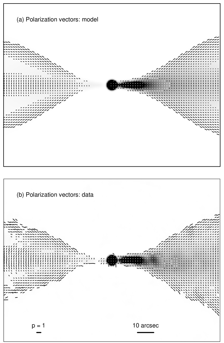
Figure 10: Vectors with lengths proportional to the degree of polarization, $p$, and directions along the apparent magnetic field, superimposed on grey-scales of total intensity. The resolution is 2.35 arcsec and vectors are plotted every 1.5 arcsec. The polarization and angular scales are indicated by the labelled bars in the lower panels and the areas plotted are the same as those in Figs 3 and 8. Vectors are plotted only where $I>5\sigma_{I}$ and $P>3\sigma_{P}$ (Table 1). (a) model; (b) data.

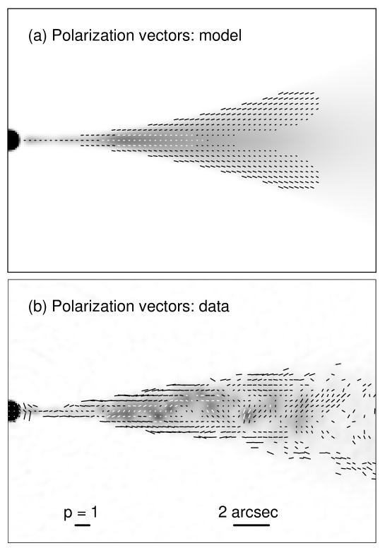
Figure 11: Vectors with lengths proportional to the degree of polarization, $p$, and directions along the apparent magnetic field, superimposed on grey-scales of total intensity. The resolution is 0.4 arcsec FWHM and vectors are plotted every 0.4 arcsec. The polarization and angular scales are indicated by the labelled bars in the lower panels and the areas plotted are the same as those in Figs 4 and 8. Vectors are plotted only where $I>5\sigma_{I}$ and $P>3\sigma_{P}$ (Table 1). (a) model; (b) data.

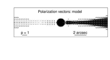
Figure 12: Vectors with lengths proportional to the degree of polarization, $p$, and directions along the apparent magnetic field, superimposed on grey-scales of total intensity for the model at a resolution of 0.4 arcsec FWHM. The polarization and angular scales are indicated by the labelled bars and the inner $\pm$8 arcsec is shown. Vectors are plotted if $I>2$ $\mu$Jy (beam area)^-1 (cf. Fig. 11). This plot shows the model polarization structure of the counter-jet near the nucleus, including the null at 3.6 arcsec and the region of transverse apparent field closer in. The data are not plotted for comparison at this resolution because the signal-to-noise ratio in the counter-jet is too low, but these features are qualitatively consistent with the low-resolution images (Figs 8b,c and  10b).

Fig. 8 compares the model and observed degrees of polarization, $p$ at resolutions of 2.35 arcsec (a – c) and 0.4 arcsec (d – f). The values of $p$ are represented as grey-scales and as profiles along the jet axis. Fig. 9 compares the average transverse profiles of the degree of polarization at distances from the nucleus between 45 and 66.5 arcsec. Finally, Figs 10, 11 and 12 represent both the value of $p$ (vector length) and the direction of the apparent magnetic field (vector direction) at the two resolutions.

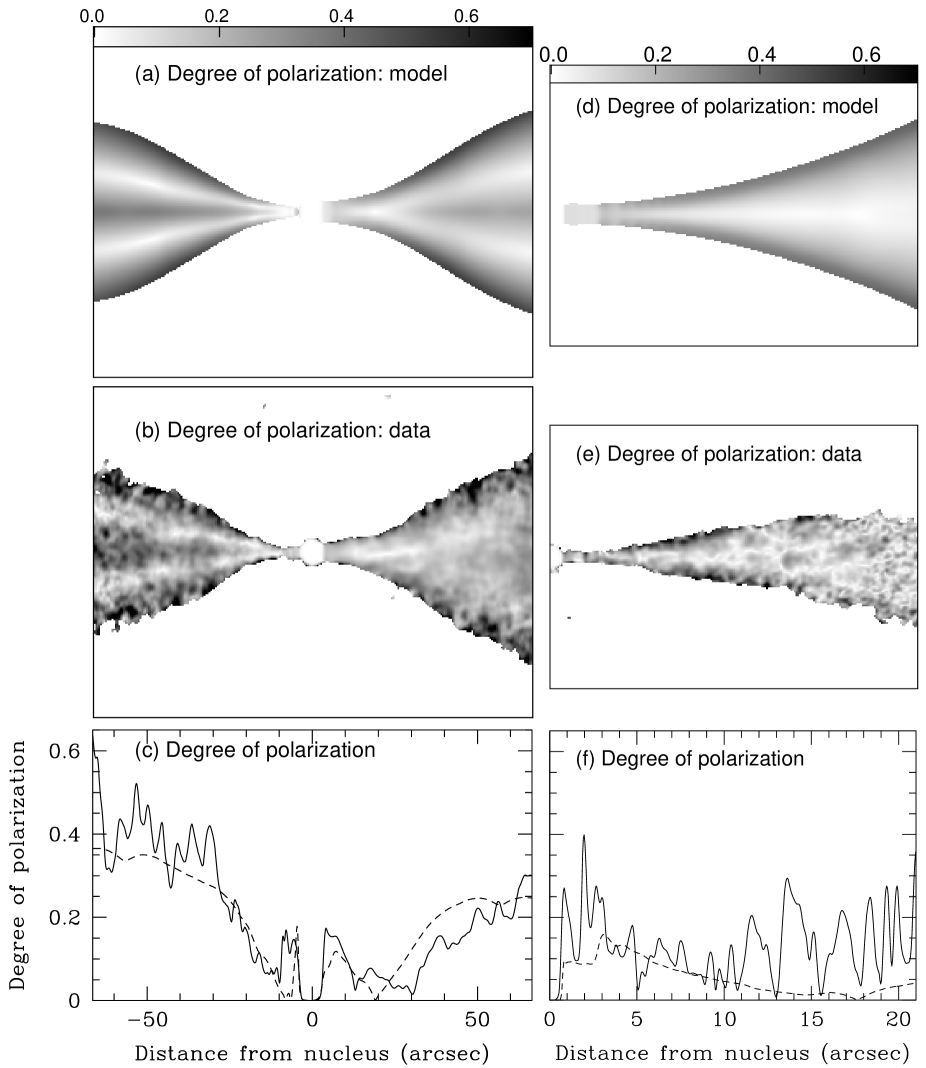
Figure 8: A comparison of the degree of polarization, $p$, for model and data. (a) and (b) grey scales of $p$ at 2.35 arcsec resolution in the range 0 – 0.7. (c) Profiles of $p$ along the jet axis for the data (full line) and model (dashed). Panels (a) – (c) show the inner 66.5 arcsec of each jet. (d) and (e) grey-scales of $p$ for the main jet at 0.4 arcsec resolution. (d) model, (e) data. (f) Profile of $p$ along the axis for the main jet. Panels (d) – (f) show the inner 21 arcsec of the main jet. The data are blanked only if $I<5\sigma_{I}$, to avoid discriminating against areas of low $p$. The models are not blanked.

The following polarization features are well described by the model:

1. The degree of polarization in the brightest portion of the main jet has a V-shaped structure, with high polarization close to the edges and low polarization on-axis (Figs 8d and e).

2. Both jets show a high degree of polarization at their edges, with the apparent magnetic field parallel to the edge everywhere (Fig. 10).

3. The main jet shows a transition from longitudinal to transverse apparent field on-axis at a distance of $\approx$30 arcsec from the nucleus whereas the counter-jet shows transverse apparent field on-axis everywhere there is adequate signal (Fig. 10).

4. Within $\approx$3 arcsec of the nucleus, the counter-jet has a transverse apparent field with $p\approx$ 0.15 – 0.2. At 3.6 arcsec, there is a polarization minimum (consistent with zero); at larger distances the degree of polarization increases with distance (Fig. 8c). The polarization direction is difficult to see in Fig. 10(a), where the model is blanked if $I<5\sigma_{I}$ or $P<3\sigma_{P}$ to match the data. Close to the nucleus, the counter-jet has discrete knots of emission with detectable polarization; the model is smoother, has a lower peak intensity and is totally blanked. For this reason Fig. 12 shows model polarization vectors close to the nucleus with minimal blanking.

5. The counter-jet shows a much more pronounced ridge of high, transverse polarization on-axis than does the main jet (Fig. 9).

6. The on-axis polarization of the counter-jet is systematically higher than that of the main jet at distances $>$30 arcsec, where both show transverse apparent field (Fig. 8c).

4.3 Features that are not fitted well

As discussed in more detail by Worrall et al. (in preparation), the bright region of the main jet is resolved into complex knots and filaments and its structure is clearly not axisymmetric in either total intensity or linear polarization (the same is almost certainly true of the counter-jet, but we see only its brightest few knots). Our model fits the inner jets with a smooth brightness distribution of the correct mean value, but there are large local deviations. An inevitable consequence is that there are fluctuations in sidedness ratio, which we cannot fit. We emphasize that relying on the sidedness ratio alone to derive jet properties is dangerous: it is necessary to average the intensity over a region large enough to contain many fluctuations, but small compared with variations in the underlying flow. This may not always be possible. The intensity fits close to the nucleus have two problems which may be due to small-scale fluctuations:

1. There is significant emission from the counter-jet close to the nucleus, (Fig. 5) and the sidedness ratio derived by integrating over the emission between 0.8 and 1.5 arcsec from the nucleus at 0.4 arcsec resolution is 6.65, much smaller than is seen further out (Fig. 3g). In principle, such an increase of sidedness cannot occur in a monotonically decelerating jet and our model fails to reproduce it. We return to this point in Section 5.3.2.

2. The first brightening of the counter-jet is slightly, but significantly further from the nucleus than the corresponding feature in the main jet: the model predicts that they should both brighten at the same place (Fig. 3d). This effect causes the huge peak in observed sidedness ratio seen in Fig. 3(g). It almost certainly results from the coincidence of a knot in the main jet with a minimum in the counter-jet at $\approx$9 arcsec from the nucleus (Fig. 5).

A related problem causes a discrepancy between the predicted and observed degrees of polarization observed on-axis in the bright region of the main jet: this appears to be due to filaments with aligned apparent fields crossing the jet axis at an oblique angle (Fig. 11b). At high resolution, the model fits the lower bound of the polarization profile quite well (Fig. 8f).

In addition to small-scale, non-axisymmetric structure (which affects all of the sources we have studied at some level) the model of NGC 315 also fails to fit two other features.

1. The on-axis sidedness ratio is slightly higher than predicted at large distances from the nucleus, leading to a larger contrast in sidedness ratio between centre and edge than is predicted by the model (Figs 3 and 7). This may indicate that the transverse velocity profile is more complex than we assume, and we discuss this point further in Section 5.3.3.

2. The average transverse polarization profile for the main jet is slightly flatter than predicted by the model at distances between 45 and 66.5 arcsec from the nucleus (Fig. 9).

5 Physical parameters

5.1 Summary of parameters

In this section, all distances in linear units are measured in a plane containing the jet axis (i.e. not projected on the sky). The parameters of the best-fitting model and their approximate uncertainties are given in Table 3.

Table 3: Fitted parameters and error estimates.

Quantity	Symbol	opt	min	max
Angle to line of sight (degrees)	$\theta$	37.9	36.1	40.7
Geometry
Boundary position (kpc)	$r_{0}$	49.18	47.37	50.61
Jet half-opening angle (degrees)	$\xi_{0}$	3.75	0.08	6.52
Width of jet at outer boundary (kpc)	$x_{0}$	12.71	12.10	13.37
Velocity
Boundary positions (kpc)
inner	$\rho_{\rm v_{1}}$	7.59	4.28	10.10
outer	$\rho_{\rm v_{0}}$	18.07	16.24	19.74
On $-$  axis velocities / $c$
inner	$\beta_{1}$	0.88	0.77	0.99
outer	$\beta_{0}$	0.38	0.35	0.41
Fractional velocity at edge of jet
inner	$v_{1}$	0.79	0.59	1.05
outer	$v_{0}$	0.58	0.45	0.71
Emissivity
Boundary positions (kpc)
inner	$\rho_{\rm e_{1}}$	2.52	0.00	3.22
2	$\rho_{\rm e_{2}}$	3.53	2.70	4.75
3	$\rho_{\rm e_{3}}$	9.41	9.14	9.73
4	$\rho_{\rm e_{4}}$	10.05	9.71	10.30
On $-$  axis emissivity exponents
inner	$E_{\rm in}$	3.15	$<$	4.00
2	$E_{\rm rise}$	0.03	$<$	2.34
3	$E_{\rm mid}$	2.79	2.33	3.18
4	$E_{\rm fall}$	10.39	6.45	13.47
5	$E_{\rm out}$	2.87	2.72	3.04
Fractional emissivity at edge of jet
inner boundary	$e_{1}$	1.01	0.41	2.12
boundary 3	$e_{0}$	0.45	0.30	0.64
B-field
Boundary positions (kpc)
inner	$\rho_{\rm B_{1}}$	0.46	0.00	6.47
outer	$\rho_{\rm B_{0}}$	25.79	20.85	31.73
RMS field ratios
radial/toroidal
inner region axis	$j_{1}^{\rm axis}$	1.12	0.54	1.71
inner region edge	$j_{1}^{\rm edge}$	0.45	0.03	0.82
outer region axis	$j_{0}^{\rm axis}$	0.61	0.08	0.91
outer region edge	$j_{0}^{\rm edge}$	0.20	0.00	0.39
longitudinal/toroidal
inner region axis	$k_{1}^{\rm axis}$	1.43	1.18	1.70
inner region edge	$k_{1}^{\rm edge}$	0.95	0.77	1.14
outer region axis	$k_{0}^{\rm axis}$	0.97	0.79	1.19
outer region edge	$k_{0}^{\rm edge}$	0.37	0.19	0.52

Figure 9: Average transverse profiles of the degree of polarization for the main and counter-jets at a resolution of 2.35 arcsec. The profiles are generated by averaging along radii between 45 and 66.5 arcsec from the nucleus and plotting against angle from the jet axis. In both panels, the data are represented by full lines and the model by dashed lines. (a) main jet, (b) counter-jet.

5.2 Geometry and angle to the line of sight

The best-fitting model has an angle to the line of sight of $\theta=38^{\circ}\pm 2^{\circ}$, consistent with the range $30^{\circ}\la\theta\la 40^{\circ}$ estimated by Giovannini et al. (2001) from the core prominence, proper-motion measurements and jet/counter-jet intensity on pc scales (the last using an isotropic emission model). The shape of the outer edge is shown in Fig. 13(a). The initially well-collimated jets flare in the inner 15 kpc to a maximum opening angle $\approx$20^∘, which is maintained over most of the rest of the modelled region. The cubic fit to the jet radius requires that a conical region should start at a distance of 49 kpc from the nucleus (90 arcsec in projection on the sky) and have an opening angle $<$6^∘. This is consistent with the observed appearance of the jets at larger distances (Fig. 1), taking into account the bends at 70 arcsec. NGC 315’s jets are therefore similar to those in other objects in recollimating to become almost cylindrical, but only after the slight bends which limit our modelling. On scales $\ga$500 arcsec in projection, there is a second rapid expansion (Willis et al., 1981; Bridle, 1982).

5.3 Velocity

5.3.1 Model fits

The boundaries between the three velocity regimes are plotted, together with their errors, in Fig. 13(a). The on-axis velocity profile, shown by the full line in Fig. 13(b), is fit with a constant value of $\beta=0.88\pm 0.1$ over the inner 7 kpc, but this value is determined primarily by the data at distances $\ga$2.5 kpc, where the jet widens and brightens. Between 7 and 20 kpc, the jet decelerates uniformly, reaching a well-constrained asymptotic speed that is still appreciably relativistic ($\beta=0.38\pm 0.03$) and persists to the end of the modelled region at 38 kpc. The best-fitting velocity at the jet edge is slower than the on-axis value, the edge/on-axis ratio varying from $0.8\pm 0.2$ close to the nucleus to $0.58\pm 0.13$ at large distances. A constant value of 0.6 – 0.7 would fit quite well everywhere, but a constant (top-hat) transverse profile is also consistent with the data close to the nucleus. The full velocity field is shown as contours in Fig. 14.

5.3.2 Evidence for acceleration?

On pc scales, both the jet/counter-jet ratio and the apparent component speed increase with distance from the nucleus (Cotton et al., 1999; Giovannini et al., 2001), although no changes in velocity have yet been detected in any individual component. The velocities derived from the measurements in Cotton et al. (1999), but taking our best-fitting inclination angle of $\theta=37.9^{\circ}$ and $H_{0}$ = 70 $\rm{km\,s^{-1}\,Mpc^{-1}}$, are plotted in Fig. 15. The velocities from $I_{\rm j}/I_{\rm cj}$ are systematically higher than those from component motions at the same distance from the nucleus for this Hubble Constant. An estimate from $I_{\rm j}/I_{\rm cj}$ for our 0.4 arcsec image between 0.8 and 1.5 arcsec from the core in projection ($\approx$0.6 kpc along the axis) is also included. This assumes (as in Cotton et al. 1999) that the rest-frame emission is isotropic, so that:

$$\frac{I_{\rm j}}{I_{\rm cj}}=\left(\frac{1+\beta\cos\theta}{1-\beta\cos\theta}\right)^{2+\alpha}$$

We also plot the results of our model fits for the centre and edge of the jet for distances $>$2.5 kpc, where they are well determined. Aside from the low value at $\approx$0.6 kpc, the velocities are consistent with acceleration from $\beta\approx 0.7$ at 1 pc to $\beta\approx 0.95$ at 10 pc, an approximately constant velocity between 10 pc and 8 kpc and deceleration as described earlier. M 87 (Reid et al., 1989; Biretta, Zhou & Owen, 1995; Biretta & Junor, 1995; Junor & Biretta, 1995) and Cen A (Tingay, Preston & Jauncey, 2001; Hardcastle et al., 2003) also show component speeds which increase from pc to kpc scales. Similarly, NGC 6251 has been suggested as an example of an accelerating flow because its jet/counter-jet ratio increases with distance (Sudou et al., 2000), although the detection of a counter-jet on pc scales was not confirmed by Jones & Wehrle (2002). Two possible mechanisms for increase of velocity on pc scales are thermal acceleration of proton-electron plasma (Melia, Liu & Fantuzzo, 2002) and magnetic driving (Vlahakis & Königl, 2004).

As noted by Cotton et al. (1999), it is unclear whether the apparent acceleration on pc scales occurs because the bulk flow accelerates or because we see different parts of a jet stratified in velocity at different distance from the core. An acceleration process which only reaches a speed of $\beta\approx 0.7$ at 1 pc is impossible to reconcile with FR I radio galaxies being the parent population of TeV blazars, as highly relativistic ($\Gamma\ga$ 10 – 20) flow is required on 0.1-pc scales in the latter class to produce the observed $\gamma$-ray emission. Velocity gradients have indeed been inferred on sub-pc scales to explain the simultaneous observations of slowly-moving radio components and highly variable TeV emission in blazars (Ghisellini, Tavecchio & Chiaberge, 2005). Similarly, although the anomalously small velocity estimate at 0.6 kpc in NGC 315 might well result from a random intensity fluctuation, 3C 31 (LB) and B2 0326+39 (CL) also show lower sidedness ratios close to the nucleus than at the flaring point, suggesting that the material contributing the bulk of the emission in the faint region at the jet base really is slower than that further out, where our models are well constrained. We cannot resolve the transverse velocity structure of the jets in their innermost regions, so it is possible that they have very fast central spines whose emission is Doppler dimmed on both sides of the nucleus and that the visible emission comes from much slower surface layers. Rapid deceleration of the spine to a speed $\beta_{1}\approx 0.9$ at 2.5 – 3.5 kpc from the nucleus would make it visible, dominating the emission and causing the sidedness ratio to rise, as suggested for 3C 31 by LB. Further from the nucleus, there are local minima in the sidedness ratio at 35 and 50 arcsec, separated by a maximum at 40 arcsec (Fig. 3j). These could be interpreted as changes in velocity in the range $0.32<\beta_{0}<0.42$, but they show no coherent pattern, so we believe that they probably reflect intrinsic differences between the two jets.

5.3.3 Transverse velocity profile

The discrepancy between the predicted and observed transverse profiles of jet/counter-jet sidedness ratio (Fig. 7) provides the first evidence that the Gaussian and spine/shear-layer velocity profiles we have employed so far may be oversimplified. The effect, which is present in all three average profiles shown in Fig. 7, is that the sidedness ratio has a sharp peak within $\approx 5^{\circ}$ of the jet axis, drops abruptly at $\approx 10^{\circ}$ and has a flatter wing at the edge of the jet. The type of velocity profile which could produce the observed results would have a central spine of high velocity ($\beta\approx 0.5$) surrounded in turn by a relatively narrow shear layer and an outer wing with $\beta\approx 0.2$. There are important implications for the evolution of the magnetic field, which would be sheared only over a narrow range of radii, rather than the majority of the jet, and for the physics of the deceleration process. The other sources we have studied (LB, CL) show no systematic discrepancies, but are less well resolved than NGC 315 in regions where they have significant changes in sidedness from axis to edge.

5.4 Emissivity

The boundaries between the emissivity regions, with their errors, are shown in Fig. 13(c) and the on-axis profile of $n_{0}B^{1+\alpha}$, derived from the emissivity, is plotted as the heavy, full line in Fig. 13(d). $n_{0}$ and $B$ are in SI units. The emissivity profile at distances $\la$3.5 kpc from the nucleus is poorly constrained (Table 3). Again, this is partly because the jets are faint and poorly resolved, but more as a consequence of the poor fit to the counter-jet (Sections 4.3), which causes the $\chi^{2}$ values to change very little as the model parameters are varied. The profile plotted in Fig. 13(d) is essentially determined by the brightness distribution of the main jet for distances $<$3.5 kpc. We model it as an inner region with a slope $E_{\rm in}\approx 3$ ($<$2.5 kpc) followed by a transition zone with a much flatter slope $E_{\rm rise}\approx 0$ from 2.5 – 3.5 kpc. The sudden increase in the observed surface brightness of the main jet (Fig. 4) is then produced by a rapid expansion of the jet at roughly constant velocity and emissivity. The emissivity profile for the bright, well-resolved sections of the jets can be divided into two power-law sections, with indices of $E_{\rm mid}=2.8$ (3.5 – 9.4 kpc) and $E_{\rm out}=2.9$ ($>$10.1 kpc). These are separated by a second short transition zone over which the emissivity drops by a factor $\approx$2, modelled as a very steep power law with index $E_{\rm fall}\approx 10.4$ between 9.4 and 10.1 kpc; this might also be represented as a discontinuity. The bright region (3.5 – 9.4 kpc) contains complex, non-axisymmetric and knotty structure (Figs 4b and 11b), whose average is represented well but whose details are not. The outer section is, by contrast, relatively smooth. There is no evidence for any transverse variation of emissivity at the start of the bright region, although this is poorly constrained. In the outer section the edge emissivity is about half of its on-axis value (a profile of $n_{0}B^{1+\alpha}$ at the jet edge is shown as the light, full line in Fig. 13c).

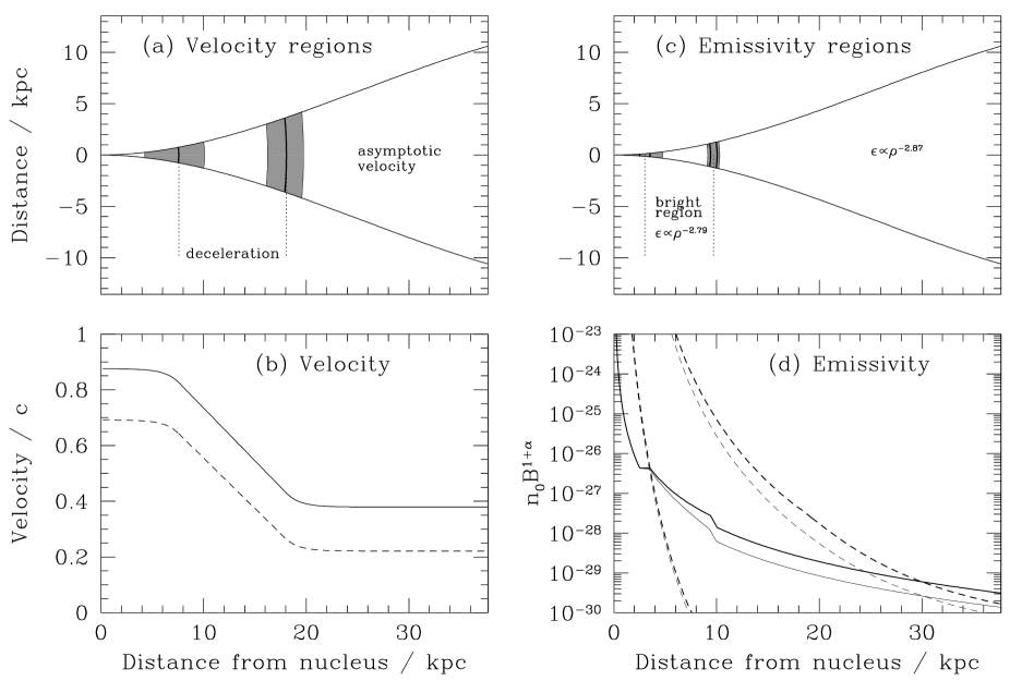
Figure 13: Panels (a) and (c): sketches showing the relative positions of the boundary surfaces between velocity and emissivity regions. The boundaries are defined in Table 2 and their positions for the best fitting model are given in Table 3. The full vertical curves indicate the boundaries and the shaded areas their allowed ranges, also from Table 3. (a) Velocity. The regions of approximately uniform deceleration and asymptotic outer velocity are marked. (c) Emissivity. The region of enhanced emissivity between 3 and 10 kpc is indicated. (b) and (d): profiles of intrinsic parameters along the jets in the rest frame. (b) the velocity profile along the jet axis (solid line) and jet edge (dashed line). (d) $n_{0}B^{1+\alpha}$ derived from the emissivity, with $n_{0}$ and $B$ in SI units. Solid line: model; dashed line, adiabatic approximation with the magnetic-field structure expected from flux freezing. The adiabatic model curves are plotted twice, normalized to match the model at 3.5 and 30 kpc from the nucleus, respectively. The heavy lines show the on-axis profiles; thin lines the edge profiles.

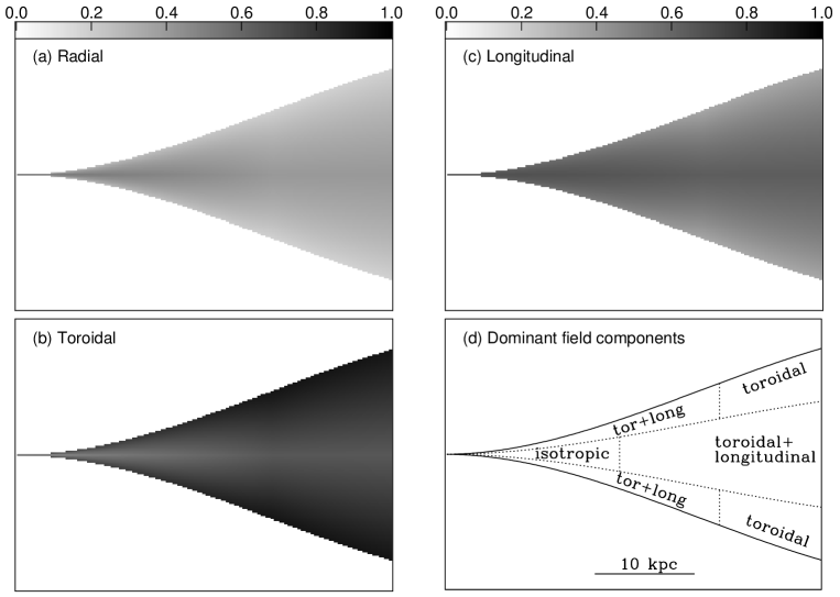
Figure 16: Panels (a) – (c): grey-scales of the fractional magnetic-field components. (a) radial, $\langle B_{r}^{2}\rangle^{1/2}/B$; (b) toroidal $\langle B_{t}^{2}\rangle^{1/2}/B$; (c) longitudinal $\langle B_{l}^{2}\rangle^{1/2}/B$. $B=\langle B_{r}^{2}+B_{t}^{2}+B_{l}^{2}\rangle^{1/2}$. (d) Sketch of the dominant field components at different locations in the jet, as deduced from the model fits.

The bright region is clearly differentiated from the rest because its emissivity is a factor of 2 higher than expected from a smooth extrapolation between smaller and larger distances (Fig. 13d). We also resolve the inner boundary of this region in 3C 31 and B2 0326+39 (LB, CL), modelling it as a discontinuous increase in emissivity. The bright region comes to an equally abrupt end, marked by an almost discontinuous drop in emissivity in NGC 315 (Fig. 13d) and B2 0326+39 (fig. 16c of CL). B2 1553+24 may show a similar feature, but is less well resolved (fig. 18c of CL). In all three sources, the drop in emissivity occurs well before the jets recollimate. 3C 31 does not show any sharp decrease in emissivity.

The phenomenon of sudden brightening and expansion at a flaring point close to the nucleus is very common in FR I jets (e.g. Parma et al. 1987), but the equally sudden emissivity drop at the end of the bright region has only become apparent from our modelling of NGC 315 and B2 0326+39. In both sources, the drop is located just after the start of the rapid deceleration ($\rho=\rho_{v_{1}}$; see Table 3) and coincides with it to within the errors. This association reinforces the argument that dissipation in FR I jets, leading to enhanced radio emission and the production of synchrotron radiation at much higher frequencies, is associated mainly with their fastest parts (Laing & Bridle, 2004).

5.5 Magnetic-field structure

The variation of magnetic-field structure is illustrated by Fig. 16, which shows grey-scales of the fractional field components: radial, $\langle B_{r}^{2}\rangle^{1/2}/B$, toroidal, $\langle B_{t}^{2}\rangle^{1/2}/B$ and longitudinal, $\langle B_{l}^{2}\rangle^{1/2}/B$ as defined in Section 3.3.3. Profiles of these quantities as functions of distance along the jet axis, $z$, are plotted in Fig. 17 for on-axis and edge streamlines. All three components vary slowly out to a distance of 25 kpc, after which they remain constant. The errors on the radial component are much larger than on the other two. On-axis, all three components are initially roughly equal (i.e. the field is on average isotropic); further out the toroidal component increases and the radial and longitudinal components decrease. At the edge of the jet, the toroidal component is always the largest, and dominates over the other two at large distances (Fig. 17d). The main field components in different parts of the jets are shown schematically in Fig. 16(d).

It is difficult to assess the uncertainties in the field component ratios from the error estimates in Table 3, so each panel of Fig. 17 includes a shaded area defining the region which the profile could occupy if any one of the six free parameters defining it is varied up to its quoted error.

The field structure we infer for the jets in NGC 315 within $\approx$15 kpc of the nucleus shows some similarities to that suggested for M 87 by Perlman et al. (1999). In our model for NGC 315, the best estimate for the field configuration on-axis in this region is roughly isotropic (although there are large uncertainties in the magnitude of the radial component; Fig. 17b); at any rate, the radial component is larger on-axis than at the edge, where longitudinal and toroidal components dominate. Perlman et al. (1999) suggest that the perpendicular component of apparent field in M 87 is larger close to the axis and is associated preferentially with the optical knots whereas the (mainly radio) edge emission has its apparent field aligned with the jet axis. In our picture, the aligned apparent field at the edge comes from the projection of intrinsically longitudinal and toroidal components and the radial component is significant only on-axis.

Finally, we note that symmetry of the average transverse intensity and polarization profiles rules out a global helical field unless the jet is observed side-on in the rest frame of the emitting material (Laing, 1981). The condition for side-on emission in the rest frame for the approaching jet in NGC 315, $\beta=\cos\theta=0.79$, is roughly satisfied before the jets decelerate, but not for distances $\ga$10 kpc from the nucleus. In the counter-jet, the condition can never hold. The intensity and polarization profiles at large distances (Figs 6 and  9) are extremely symmetrical, particularly in the counter-jet, and we can rule out globally-ordered helical fields on these scales. A configuration in which the toroidal component is vector-ordered but the longitudinal component has many reversals would give identical brightness and polarization distributions to those we calculate for a fully disordered, anisotropic field and we cannot rule out such a field configuration.

Figure 14: Contours of the model velocity field. The contours are at intervals of 0.05 in the range $\beta=$ 0.25 – 0.85.

Figure 15: A comparison of velocity estimates on pc and kpc scales, plotted against distance from the nucleus (note the logarithmic scale). We assume that $\theta=37.9^{\circ}$ everywhere. Filled squares: velocities from proper motions; open squares: velocities from jet/counter-jet ratios (both from Cotton et al. 1999, but with our choice of Hubble Constant). The open triangle shows the velocity derived from the jet/counter-jet ratio at 0.4 arcsec resolution close to the nucleus. All velocity estimates from intensity ratios alone are calculated for isotropic emission in the rest frame. The full and dotted lines show our model fits for the centre and edge of the jets, respectively. They are plotted only for distances $>$2.5 kpc, where they are well constrained (see Section 5.3.2).

5.6 Flux freezing and adiabatic models

In this section, we follow Laing & Bridle (2004) in referring to our detailed fits as free models in order to distinguish them from the adiabatic models considered here. Given the assumption of flux freezing in a jet without a transverse velocity gradient, the magnetic field components evolve according to:

$$B_{r} \propto (x\beta\Gamma)^{-1}$$

$$B_{t} \propto (x\beta\Gamma)^{-1}$$

$$B_{l} \propto x^{-2}$$

in the quasi-one-dimensional approximation, where $x$ is the radius of the jet (Baum et al., 1997). The dashed lines in Fig. 17 show the predicted evolution of the field components, normalized to match the models at a distance of 30 kpc from the nucleus. The evolution of the longitudinal and toroidal components is qualitatively as expected but quantitatively inconsistent: the longitudinal/toroidal ratio decreases with distance, but much less rapidly than predicted. Shear will tend to slow the decline of the longitudinal component, however, so an axisymmetric adiabatic model of the type described by Laing & Bridle (2004) may provide a better description. If the transverse velocity profile indeed has the form suggested by the average sidedness profile (Fig. 7, Section 5.3.3), then shear would be localised at intermediate radii, a more complex situation than that considered by Laing & Bridle (2004). In contrast, the evolution of the on-axis radial component, is qualitatively inconsistent with flux freezing in any simple axisymmetric, laminar-flow model: the radial/toroidal field ratio decreases with distance instead of remaining constant. Anomalous behaviour of the radial component also occurs in 3C 31 and B2 0326+29 (LB, CL).

Assuming that the radiating electrons suffer only adiabatic losses, and again adopting the quasi-one-dimensional approximation, the emissivity is:

$$\epsilon\propto(x^{2}\beta\Gamma)^{-(1+2\alpha/3)}B^{1+\alpha}$$

(Baum et al., 1997; Laing & Bridle, 2004). $B$ can be expressed in terms of the parallel-field fraction $f=\langle B_{l}^{2}\rangle^{1/2}/B$ and the radius $\bar{x}$, velocity $\bar{\beta}$ and Lorentz factor $\bar{\Gamma}$ at some starting location using equation 8 of Laing & Bridle (2004):

$$B\propto\left[f^{2}\left(\frac{\bar{x}}{x}\right)^{4}+(1-f^{2})\left(\frac{\bar{\Gamma}\bar{\beta}\bar{x}}{\Gamma\beta x}\right)^{2}\right]^{1/2}$$

We compare the adiabatic and free model emissivity profiles, normalized at distances of 3.5 and 30 kpc, in Fig. 13(d). In the innermost region, where the fit to the counter-jet is poor, the slope $E_{\rm in}$ of the emissivity variation is essentially unconstrained (Section 5.4 and Table 3). Everywhere else there is a clear difference: the emissivity predicted by the adiabatic approximation falls more rapidly than that derived from the free model. Dissipative processes must occur to accelerate the radiating particles where X-ray synchrotron emission is detected, i.e. at distances up to at least 15 arcsec in projection, corresponding to 8 kpc in the jet frame (Worrall, Birkinshaw & Hardcastle, 2003; Donato, Sambruna & Gliozzi, 2004). The failure of adiabatic models is therefore inevitable at these distances, but our results suggest that they are inadequate to describe the emissivity variations anywhere in the modelled region. The discrepancies are probably too large to be accounted for by field amplification due to shear in a laminar, axisymmetric, adiabatic model of the type developed by Laing & Bridle (2004). In general, we have found that adiabatic models only come close to fitting the brightness distributions of FR I jets after they have recollimated (LB, CL, Laing & Bridle 2004) and we have not modelled this region in NGC 315.

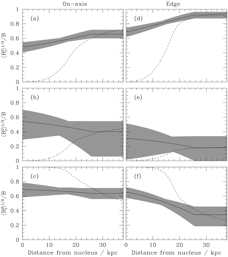
Figure 17: Profiles of magnetic-field components along the axis of the jet (panels a – c) and its edge (panels d – f). The solid lines show the best-fitting model, the shaded areas the uncertainties derived from the limits in Table 3 and the dashed lines the profiles expected for a magnetic field frozen into the flow. The profiles for a passively convected field are normalized to the free model predictions at a distance of 30 kpc from the nucleus. (a) and (d) toroidal; (b) and (e) radial; (c) and (f) longitudinal.

6 Summary and further work

6.1 Summary

We have shown that the synchrotron emission from the flaring region of the jets in the FR I radio galaxy NGC 315 can be fit accurately on the assumption that they are intrinsically symmetrical, axisymmetric, relativistic decelerating flows. The functional forms we use to describe the geometry, emissivity, velocity and magnetic-field structure are very close to those developed in our previous work (LB, CL). The geometry and the relative locations of the emissivity and velocity regions are very similar to those in two of the other sources we have modelled (3C 31 and B2 0326+39), except that all of the physical scales in NGC 315 are larger by a factor of $\approx$5.

6.1.1 Geometry

We have modelled only the flaring region within 70 arcsec (in projection) of the nucleus, as the jets bend shortly thereafter. As in other objects we have studied, the radius $x$ of its outer isophote is well fitted by the expression $x=a_{2}z^{2}+a_{3}z^{3}$, where $z$ is the distance from the nucleus along the axis. The jets make an angle of $\theta=38^{\circ}\pm 2^{\circ}$ with the line of sight, so the size of the region we model is 38 kpc and the intrinsic length of the flaring region is $\approx$50 kpc, much larger than in the other objects.

6.1.2 Velocity

The velocity is well constrained from 2.5 kpc outwards, where the jet brightens rapidly (the flaring point). From 2.5 to $\approx$8 kpc the on-axis speed is consistent with a constant value of $\beta=0.88\pm 0.11$. This is very similar to the values derived at the flaring point for the other sources we have modelled in detail (LB, CL) and from a statistical analysis of sidedness ratios for a larger sample (Laing et al., 1999). An anomalous region of low jet/counter-jet sidedness ratio $<$2.5 kpc from the nucleus appears to indicate a lower velocity there, but the jets are faint and poorly resolved, so this could be due to local fluctuations in the jet or counter-jet brightness. Between 8 and 18 kpc the jet decelerates uniformly to an asymptotic speed of $\beta=0.38\pm 0.03$ which is maintained until the end of the modelled region. B2 0326+39 and B2 1553+24 show velocity profiles of identical form, but with lower asymptotic velocities (CL), whereas 3C 31 continues to decelerate slowly on larger scales (LB). NGC 315 shows a significant transverse velocity gradient, with an edge velocity consistent with 0.6 – 0.7 of the on-axis value everywhere, as in the other sources. There are hints from the sidedness ratio at large distances that our assumed (Gaussian) form for the transverse velocity profile may be inadequate, and that a profile with a central spine ($\beta\approx 0.5$) separated from an outer sheath ($\beta\approx 0.2$) by a relatively narrow shear layer may provide a better fit.

6.1.3 Emissivity

The emissivity profile along the jets is modelled as three main power-law sections with slopes of $-3.5$ (0 – 2.5 kpc; very poorly constrained), $-2.8\pm 0.5$ (3.5 – 9.4 kpc) and $-2.9\pm 0.2$ (9.4 – 38 kpc). These are separated by short transition zones, also modelled as power laws. The first of these (2.5 – 3.5 kpc) is roughly constant and represents the brightening of the jet as a very rapid expansion at constant emissivity. The second, from 9.4 – 10.1 kpc is very steep and describes an almost discontinuous drop in emissivity by a factor of 2. Simple adiabatic models predict too steep an emissivity decline, as we also found for the flaring regions of other jets. The emissivity is centre-brightened where its transverse variation is well constrained.

6.1.4 Magnetic field

To fit the polarization structure of the jets, transverse variation of field structure had to be included in our models. On axis, the field is roughly isotropic $\la$10 kpc from the nucleus, but the radial component declines, leaving an equal mix of longitudinal and toroidal field by the end of the modelled region. At the edge of the jets, the radial component is small and the field configuration evolves from an equal mix of longitudinal and toroidal close to the nucleus to almost pure toroidal at large distances. From the symmetry of the transverse intensity and polarization profiles, particularly in the outer parts of the jets, we infer that there cannot be a significant, globally-ordered helical field. All three components could have many reversals or the toroidal component could be globally ordered, provided that the other two are not. The evolution of the radial field component along the jets is not consistent with flux freezing in our assumed velocity field. That of the toroidal and longitudinal components is qualitatively as expected, but a more complex model, including shear, is required for a quantitative test.

6.2 Further work

We are currently acquiring VLA data for one further source, 3C 296 (Harcastle et al., 1997). We will then present model fits for all five sources using the same functional forms in order to compare their properties quantitatively. We will also investigate more complex transverse velocity profiles, as outlined in Section 5.3.3 and develop techniques to deal with slightly bent jets. Where the quasi-one-dimensional analysis presented here indicates that the adiabatic approximation is reasonable, we will fit the brightness distributions using the self-consistent adiabatic model of Laing & Bridle (2004). Once suitable X-ray observations have been made, we plan to apply the conservation-law approach of Laing & Bridle (2002b) to derive the energy and momentum fluxes of the modelled jets and their variations of pressure, density and entrainment rate with distance from the nucleus.

There are, as yet, no observations of jets in FR II sources, or in any class of source on scales $\la$1 kpc, with resolution and sensitivity adequate for detailed modelling. The advent of EVLA, e-MERLIN and broad-band VLBI should allow us to apply our techniques to more powerful (and probably faster) jets and to probe scales much closer to those on which jets are launched.

References

- (1)
- Baan (1980) Baan W. A., 1980, ApJ, 239, 433
- Baum et al. (1997) Baum S.A., O’Dea C.P., Giovannini G., Biretta J., Cotton W.B., de Koff S., Feretti L., Golombek D., Lara L., Macchetto F.D., Miley G.K., Sparks W.B., Venturi T., Komissarov S.S., 1997, ApJ, 483, 178 (erratum ApJ, 492, 854)
- Begelman (1982) Begelman M.C., 1982, in Extragalactic Radio Sources, eds. Heeschen D.S., Wade C.M., IAU Symp. 97, D. Reidel, Dordrecht, p. 223
- Begelman et al. (1984) Begelman M.C., Blandford R.D., Rees M.J., 1984, Rev. Mod. Phys., 56, 255
- Bicknell (1984) Bicknell G.V., 1984, ApJ, 286, 68
- Bicknell (1986) Bicknell G.V., 1986, ApJ, 300, 591
- Biretta & Junor (1995) Biretta J.A., Junor W., 1995, Proc. Natl. Acad. Sci., 92, 11364
- Biretta, Zhou & Owen (1995) Biretta J.A., Zhou F., Owen F.N., 1995, ApJ, 447, 582
- Bowman, Leahy & Komissarov (1996) Bowman M., Leahy J. P., Komissarov S. S., 1996, MNRAS, 279, 899
- Bridle (1982) Bridle A.H., 1982, in Extragalactic Radio Sources, eds. Heeschen D.S., Wade C.M., IAU Symp. 97, D. Reidel, Dordrecht, p. 121
- Bridle et al. (1976) Bridle A.H., Davis M.M., Meloy D.A., Fomalont E.B., Strom R.G., Willis A.G., 1976, Nature, 262, 179
- Bridle et al. (1979) Bridle A.H., Davis M.M., Fomalont E.B., Willis A.G., Strom R.G., 1979, ApJ, 228, 9
- Canvin & Laing (2004) Canvin J.R., Laing R.A., 2004, MNRAS, 350, 1342 (CL)
- Cotton et al. (1999) Cotton W.D., Feretti L., Giovannini G., Lara L., Venturi T., 1999, ApJ, 519, 108
- De Young (1996) De Young D. S., 1996, in Energy Transport in Radio Galaxies and Quasars, eds Hardee P.E., Bridle A.H., Zensus J.A., ASP Conf. Series 100, ASP, San Francisco, p. 261
- De Young (2004) De Young D.S., 2004, in X-Ray and Radio Connections, eds Sjouwerman L.O., Dyer K.K., http://www.aoc.nrao.edu/events/xraydio
- Donato, Sambruna & Gliozzi (2004) Donato D., Sambruna R.M., Gliozzi M., 2004, ApJ, 617, 915
- Fanaroff & Riley (1974) Fanaroff B.L., Riley J.M., 1974, MNRAS, 167, 31p
- Fomalont et al. (1980) Fomalont E.B., Bridle A.H., Willis A.G., Perley R.A., 1980, ApJ, 237, 418
- Giovannini et al. (2001) Giovannini G., Cotton W.D., Feretti L., Lara L., Venturi T., 2001, ApJ, 552, 508
- Ghisellini, Tavecchio & Chiaberge (2005) Ghisellini G., Tavecchio F., Chiaberge M., 2005, A&A, 432, 401
- Harcastle et al. (1997) Hardcastle M.J., Alexander P., Pooley G.G., Riley J.M., 1997, MNRAS, 288, L1
- Hardcastle et al. (2002) Hardcastle M.J., Worrall D.M., Birkinshaw M., Laing R.A., Bridle A.H., 2002, MNRAS, 334, 182
- Hardcastle et al. (2003) Hardcastle M.J., Worrall D.M., Kraft R.P., Forman W.R., Jones C., Murray S.S., 2003, ApJ, 593, 169
- Jones & Wehrle (2002) Jones D.L., Wehrle A., 2002, ApJ, 580, 114
- Junor & Biretta (1995) Junor W., Biretta J.A., 1995, AJ, 109 500
- Komissarov (1994) Komissarov S.S., 1994, MNRAS, 269, 394
- Laing (1981) Laing R.A., 1981, ApJ, 248, 87
- Laing (1988) Laing R.A., 1988, Nature, 331, 149
- Laing & Bridle (2002a) Laing R.A., Bridle A.H., 2002a, MNRAS, 336, 328 (LB)
- Laing & Bridle (2002b) Laing R.A., Bridle A.H., 2002b, MNRAS, 336, 1161
- Laing & Bridle (2004) Laing R.A., Bridle A.H., 2004, MNRAS, 348, 1459
- Laing et al. (1999) Laing R.A., Parma P., de Ruiter H.R., Fanti, R., 1999, MNRAS, 306, 513
- Linfield (1981) Linfield R., 1981, ApJ, 244, 436
- Melia, Liu & Fantuzzo (2002) Melia F., Liu S., Fantuzzo M., 2002, ApJ, 567, 811
- Morganti et al. (1997) Morganti R., Parma P., Capetti A., Fanti R., de Ruiter H.R., 1997, A&A, 326, 919
- Parma et al. (1987) Parma P., Fanti C., Fanti R., Morganti R., de Ruiter H.R., 1987, A&A, 181, 244
- Perlman et al. (1999) Perlman E.S., Biretta J.A., Zhou F., Sparks W.B., Macchetto F.D., 1999, AJ, 117, 2185
- Phinney (1983) Phinney E. S., 1983, Ph.D. Thesis, University of Cambridge
- Reid et al. (1989) Reid M.J., Biretta J.A., Junor W., Spencer R., Muxlow T., 1989, ApJ, 336, 125
- Rosen & Hardee (2000) Rosen A., Hardee P.E., 2000, ApJ, 542, 750
- Rosen et al. (1999) Rosen A., Hardee P.E., Clarke D.A., Johnson A., 1999, ApJ, 510, 136
- Sudou et al. (2000) Sudou H., et al., 2000, PASJ, 52, 989
- Tingay, Preston & Jauncey (2001) Tingay S.J., Preston R.A., Jauncey D.L., 2001, AJ, 122, 1697
- Trager et al. (2000) Trager S.C., Faber S.M., Worthey G., Gonzalez J.J., 2000, AJ, 119, 1645
- Urry & Padovani (1995) Urry C. M., Padovani P., 1995, PASP, 107, 803
- Venturi et al. (1993) Venturi T., Giovannini G., Feretti L., Comoretto G., Wehrle A.E., 1993, ApJ, 408, 81
- Wardle & Kronberg (1974) Wardle J.F.C., Kronberg P.P., 1974, ApJ, 194, 249
- Vlahakis & Königl (2004) Vlahakis N., Königl A., 2004, ApJ, 605, 656
- Willis et al. (1981) Willis A.G., Strom R.G., Bridle A.H., Fomalont E.B., 1981, A&A, 62, 375
- Worrall, Birkinshaw & Hardcastle (2003) Worrall D.M., Birkinshaw M., Hardcastle M.J., 2003, MNRAS, 343, L73
- Xu et al. (2000) Xu C., Baum S.A., O’Dea C.P., Wrobel J.M., Condon J.J., 2000, AJ, 120, 2950