Three-dimensional MHD Simulations of Jets from Accretion Disks

Abstract

We report the results of 3-dimensional magnetohydrodynamic (MHD) simulations of a jet formation by the interaction between an accretion disk and a large scale magnetic field. The disk is not treated as a boundary condition but is solved self-consistently. To investigate the stability of MHD jet, the accretion disk is perturbed with a non-axisymmetric sinusoidal or random fluctuation of the rotational velocity. The dependences of the jet velocity $(v_{z})$, mass outflow rate $(\dot{M}_{w})$, and mass accretion rate $(\dot{M}_{a})$ on the initial magnetic field strength in both non-axisymmetric cases are similar to those in the axisymmetric case. That is, $v_{z}\propto B_{0}^{1/3}$, $\dot{M}_{w}\propto B_{0}$ and $\dot{M}_{a}\propto B_{0}^{1.4}$ where $B_{0}$ is the initial magnetic field strength. The former two relations are consistent with the Michel’s steady solution, $v_{z}\propto\left(B_{0}^{2}/\dot{M}_{w}\right)^{1/3}$, although the jet and accretion do not reach the steady state. In both perturbation cases, a non-axisymmetric structure with $m=2$ appears in the jet, where $m$ means the azimuthal wave number. This structure can not be explained by Kelvin-Helmholtz instability and seems to originate in the accretion disk. Non-axisymmetric modes in the jet reach almost constant levels after about 1.5 orbital periods of the accretion disk, while all modes in the accretion disk grow with oscillation. As for the angular momentum transport by Maxwell stress, the vertical component, $\langle B_{\phi}B_{z}/4\pi\rangle$, is comparable to the radial component, $\langle B_{\phi}B_{r}/4\pi\rangle$, in the wide range of initial magnetic field strength.

1 Introduction

Astrophysical jets are one of the most important and interesting subject in astrophysics. They have been observed in various spatial scales, e.g. in young stellar objects (YSOs) (e.g., Fukui et al. 1993; Ogura 1995; Furuya et al. 1999), active galactic nuclei (e.g., Bridle & Perley 1984; Kubo et al. 1998), and X-ray binaries (e.g., Margon 1984; Mirabel & Rodriguez 1994; Kotani et al. 1996). The acceleration and collimation mechanisms of jets are still not made clear and various models have been proposed (e.g., Ferrari 1998; Meier, Koide, & Uchida 2001; Bisnovatyi-Kogan & Lovelace 2001).

One of the most promising models is magnetohydrodynamic (MHD) acceleration from accretion disks. Lovelace (1976) and Blandford (1976) first pointed out that electromagnetic force can extract energy and angular momentum from accretion disks and that the plasma is accelerated relativistically in two opposite directions. Blandford & Payne (1982) showed that a magneto-centrifugally driven outflow from a Keplerian disk is possible when an angle between the poloidal magnetic field lines and the surface of the accretion disk is less than $60^{\circ}$. They discussed self-similar solutions of the steady and axisymmetric MHD equations and the possibility of such acceleration and collimation of the flow from a cold Keplerian disk. Kudoh & Shibata (1995, 1997a) solved 1-dimensional steady and axisymmetric MHD equations and investigated properties of steady MHD jet. They found that the steady MHD jet can be divided into two classes; one is the magneto-centrifugally driven jet when the magnetic field is strong and the other is the magnetic pressure driven jet when the field is weak. The former has dependences of the jet velocity ($V_{jet}$) and mass outflow rate ($\dot{M}_{w}=dM_{w}/dt$) on magnetic energy ($E_{mg}$) as $V_{jet}\propto E_{mg}^{1/3}$, $\dot{M}_{w}\sim$ constant and the latter has dependences as $V_{jet}\propto E_{mg}^{1/6}$, $\dot{M}_{w}\propto E_{mg}^{0.5}$. This mass flux scaling law was confirmed by Ustyugova et al. (1999).

On the other hand, Uchida & Shibata (1985) and Shibata & Uchida (1986, 1987) performed time-dependent 2-dimensional axisymmetric (2.5-dimensional) MHD numerical simulations of magnetically driven jets from accretion disks. They solved the interaction between a geometrically thin rotating disk and a large-scale magnetic field that was initially uniform and vertical. Shibata & Uchida (1986) investigated the dependence of the jet velocity on the magnetic field strength. The jet velocity increases as the magnetic field strength increases in a manner similar to Michel’s scaling law (Michel 1969) but is typically of the order of the disk’s Keplerian velocity. Kudoh, Matsumoto, & Shibata (1998) showed the following results: The dependences of the jet velocity ($v_{z}$) and mass outflow rate ($\dot{M}_{w}$) on the initial magnetic field strength are approximately $v_{z}\propto\left(\Omega_{F}^{2}B_{0}^{2}/\dot{M}_{w}\right)^{1/3}\propto B_{0}^{1/3}\propto E_{mg}^{1/6}$ and $\dot{M}_{w}\propto B_{0}\propto E_{mg}^{1/2}$, where $B_{0}$ is the initial poloidal magnetic field strength and $\Omega_{F}$ is the angular velocity of the field line (the angular velocity of the footpoint on the accretion disk). These are consistent with the results of 1-dimensional steady solutions although the jet and accretion never reach a steady state. It is also obtained that the dependence of the mass accretion rate ($\dot{M}_{a}=dM_{a}/dt$) on the initial field strength is given by $\dot{M}_{a}\propto B_{0}^{1.4}\propto E_{mg}^{0.7}$.

In addition to these studies, the acceleration and collimation of the jet have been studied in the steady (e.g., Sauty, Trussoni, & Tsinganos 2004; Bogovalov & Tsinganos 2005) and nonsteady framework (e.g., Matsumoto et al. 1996; Kato et al. 2002; Krasnopolsky, Li, & Blandford 2003; see also Shibata & Kudoh 1999 for a review). In recent years, interesting simulations taking other physical processes, e.g., the magnetic diffusion (Kuwabara et al. 2000; Fendt & Čemeljić 2002; Casse & Keppens 2002, 2004), the dynamo process in the accretion disk (von Rekowski et al. 2003), the radiation force (Proga 2003) into consideration have been performed. Koide, Shibata, & Kudoh (1999) showed that a magnetically driven jet in the general relativistic MHD simulation has the characteristics similar to those of the nonrelativistic MHD jet (Shibata & Uchida 1986). These works, however, assume the axisymmetry, so that instabilities having non-axisymmetric modes are eliminated. It is very interesting whether jets are stable against the non-axisymmetric modes or not. Can jets be ejected in the same manner with the axisymmetric cases? The stability of propagating jet has been studied by taking the accretion disk as the fixed boundary condition in 2-D MHD (e.g., Ustyugova et al. 1995; Ouyed & Pudritz 1997a,b, 1999; Romanova et al. 1998; Hardee & Rosen 1999, 2002; Frank et al. 2000), 3-D MHD (Nakamura, Uchida, & Hirose 2001; Ouyed, Clarke, & Pudritz 2003; Nakamura & Meier 2004), and 3-D SPMHD (smoothed particle MHD) simulations (Cerqueira & de Gouveia Dal Pino 2001). The 3-dimensional treatment is necessary for investigating the stability of the jet against the non-axisymmetric modes.

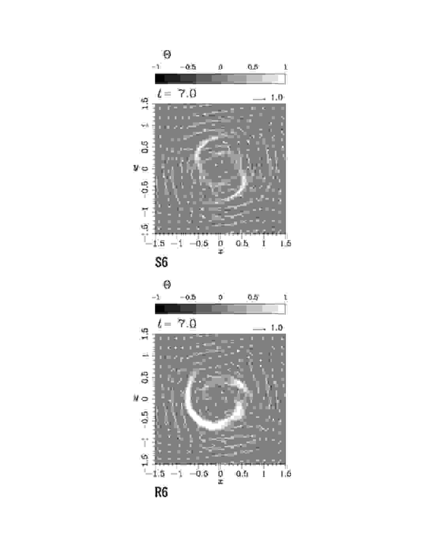
Figure 5: The distribution of $\Theta$ on the $z=1.7$ plane at $t=7.0$. The region where $\Theta=1$ means the place the disk matter exists.

Magnetically driven jets have a helical magnetic field because accretion disks twist the magnetic field by their own rotation. The generated toroidal magnetic field propagates along the magnetic field as torsional Alfvén waves. It is equivalent that current flows in the jets. The current may cause a current-driven instability and jets may be deformed. Nakamura et al. (2001) showed that the helical kink instability can explain the wiggled structures which are often observed (Krichbaum et al. 1990; Hummel et al. 1992; Conway & Murphy 1993; Roos, Kaastra, & Hummel 1993; Hutchison, Cawthorne, & Gabuzda 2001; Stirling et al. 2003). The MHD model can also explain some characteristics of polarization observations of AGN jets. Some AGN jets show ’spine+sheath’ $\bm{B}$-field structures, which consist of the transverse field in the central region and the longitudinal field becoming dominant in some regions offset from the jet axis; it is thought that the transverse field is the result of shock compression and that the longitudinal field is due to the effect of shear between a jet and a surrounding medium (e.g., Attridge, Roberts, & Wardle 1999). Gabuzda (2003), however, pointed out that jets dominated by toroidal field can display the ’spine+sheath’ structure. Uchida et al. (2004) showed this point numerically (see Figure 5a and 6a of Uchida et al. (2004)). Besides this, rotation measure gradients perpendicular to the jet axis (Asada et al. 2002; Gabuzda, Murray, & Cronin 2004; Zavala & Taylor 2005) and a distribution of rotation measure associated with the jet deformation (Feretti et al. 1999) are reproduced numerically by the MHD model (Uchida et al. 2004; Kigure et al. 2004). It can be said that these points indicate advantages of the MHD model.

Only a few 3-dimensional MHD simulations of jet formation with solving the accretion disk self-consistently have been presented (e.g., Matsumoto & Shibata 1997; Matsumoto 1999; Matsumoto & Shibata 1999; Kigure et al. 2002) although global (not adopting the shearing box approximation) 3-dimensional MHD simulations of the accretion disk around the black hole are vigorously done in recent years (e.g., Hawley 2000; Hawley & Krolik 2001; Machida & Matsumoto 2003). In this paper, we study the stability of the jet launched from the accretion disk by 3-dimensional MHD simulations. We investigate the connection between the non-axisymmetric structure in the jet and that in the disk, and compare the characteristics (e.g., the dependence of the jet velocity on the magnetic field strength) of jets found in 3-dimensional simulations with those of jets found in 2.5-dimensional simulations and in steady state models. In §2, we describe the numerical method and the initial and boundary conditions. In §3, we present results of our simulations. A discussion and conclusions are in §4 and §5.

2 Numerical Method

2.1 Assumptions and Basic Equations

We solve the following ideal MHD equations numerically:

$$\frac{\partial\rho}{\partial t}+\bm{v}\cdot\nabla\rho=-\rho\nabla\cdot\bm{v}$$ (1)

$$\frac{\partial\bm{v}}{\partial t}+\bm{v}\cdot\nabla\bm{v}=-\frac{1}{\rho}\nabla\left(p+\frac{\bm{B}^{2}}{8\pi}\right)+\frac{1}{4\pi\rho}\bm{B}\cdot\nabla\bm{B}+\bm{g}$$ (2)

$$\frac{\partial p}{\partial t}+\bm{v}\cdot\nabla p=-\gamma p\nabla\cdot\bm{v}$$ (3)

$$\frac{\partial\bm{B}}{\partial t}+\nabla\times\bm{E}=0$$ (4)

$$\bm{E}=-\bm{v}\times\bm{B}$$ (5)

where $\rho,p,\bm{v}$ are the density, pressure, and velocity of the gas respectively. $\bm{B}$ and $\bm{E}$ are the magnetic and electric field. $\gamma$ represents the ratio of specific heats and is equal to 5/3 in this paper. The gravity is assumed to be only due to a point-mass gravitational potential. This means that the gravitational acceleration, $\bm{g}$, is equal to $-\nabla\Psi$, where $\Psi=-GM/(r^{2}+z^{2})^{1/2}$. $G$ is the gravitational constant and $M$ is the mass of a central object.

2.2 Initial Conditions

As an initial condition, we assume that an equilibrium disk rotates in a central point-mass gravitational potential (e.g., Matsumoto et al. 1996, Kudoh et al. 1998). The distributions of angular momentum and pressure are assumed as follows (e.g., Abramowicz, Jaroszynski, & Sikora 1978):

$$L=L_{0}r^{a}$$ (6)

$$p=K\rho^{\Gamma}=K\rho^{1+1/n}$$ (7)

Under these simplifying assumptions, exact solution for the distribution of disk material is given by

$$\psi=-\frac{GM}{(r^{2}+z^{2})^{1/2}}+\frac{1}{2(1-a)}L_{0}^{2}r^{2a-2}+(n+1)\frac{p}{\rho}=const$$ (8)

From the value of $\psi$ at $(r,z)=(r_{0},0)$, the density and pressure distributions in the disk are derived. In this paper, $a$ and $n$ are fixed at 0 and 3 respectively.

It is also assumed that there exists a corona outside the disk with uniformly high temperature. The corona is in hydrostatic equilibrium without rotation. The density distribution of the corona is

$$\rho=\rho_{c}\rm{exp}\left[\alpha\left\{\frac{r_{0}}{(r^{2}+z^{2})^{1/2}}-1\right\}\right]$$ (9)

where $r_{0}$ is the unit length and equal to $\left(L_{0}^{2}/GM\right)^{1/(1-2a)}$. At the point where $(r,z)=(r_{0},0)$, the density of the disk is maximum. The parameter $\alpha$ is defined as $\left(\gamma V_{K0}^{2}/V_{sc}^{2}\right)$, where $V_{sc}$ is the sound velocity in the corona, $V_{K0}=(GM/r_{0})^{1/2}$ is the Keplerian velocity at radius $r_{0}$. $\rho_{c}$ is coronal density at radius $r_{0}$. $\alpha$ and $\rho_{c}/\rho_{0}$ are equal to $1.0$ and $10^{-3}$ throughout this paper, where $\rho_{0}$ is the initial density at $(r,z)=(r_{0},0)$. To distinguish the material that are initially in the disk from that in the corona, a scalar variable, $\Theta$, is introduced. The initial distribution of $\Theta$ is as follows:

$$\Theta=\left\{\begin{array}[]{ll}1&\rm{inside\ of\ the\ disk}\\ 0&\rm{outside\ of\ the\ disk}\\ \end{array}\right.$$ (12)

The inside of the disk is defined as the region where the density obtained by equation (8) is positive. The time evolution of $\Theta$ is followed by the equation,

$$\frac{d\Theta}{dt}=\frac{\partial\Theta}{\partial t}+v_{r}\frac{\partial\Theta}{\partial r}+\frac{v_{\phi}}{r}\frac{\partial\Theta}{\partial\phi}+v_{z}\frac{\partial\Theta}{\partial z}=0$$ (13)

by using the velocity obtained by solving the MHD equations.

The initial magnetic field is assumed to be uniform and parallel to the rotation axis of the disk; $\left(B_{r},B_{\phi},B_{z}\right)=\left(0,0,B_{0}\right)$.

2.3 Non-axisymmetric Perturbations in the Disk

To investigate the stability of the disk and jet system, we add the non-axisymmetric perturbation. Two types of perturbations are adopted: Either sinusoidal or random perturbation is imposed on the rotational velocity of the accretion disk. In the sinusoidal perturbation case, $\delta v_{\phi}=0.1V_{s0}\sin 2\phi$ ($0.1V_{s0}$ is about 3% of the Keplerian velocity), where $V_{s0}$ is the sound velocity at $(r,z)=(r_{0},0)$ (see Matsumoto & Shibata 1997, Kato 2002). In the random perturbation case, the sinusoidal function in the above-mentioned $\delta v_{\phi}$ is replaced with random numbers between -1 and 1. The case in which no perturbation is imposed is also calculated for a comparison.

2.4 Boundary Conditions

We impose symmetry for $\rho,v_{r},v_{\phi},B_{z}$, and $p$ but anti-symmetry for $v_{z},B_{r}$, and $B_{\phi}$ on the equatorial plane ($z=0$). The side ($r=r_{max}$) and top ($z=z_{max}$) surfaces are free boundaries for each quantity $Q$ as follows (Shibata 1983):

$$\frac{\partial\Delta Q}{\partial r}=\frac{\partial\Delta Q}{\partial z}=0$$ (14)

$$\Delta Q=Q(r,\phi,z,t+\Delta t)-Q(r,\phi,z,t)$$ (15)

On the central axis ($r=0$), the values of all physical quantities are calculated as the average of the points where $r=\Delta r$ ($\Delta r$ is the grid spacing in the $r$-direction). The $r$- and $\phi$-components of velocity and magnetic field are converted to the $x$- and $y$-components, and then the values are averaged. Therefore the velocity and the magnetic field can have non-zero $x$- and $y$-components on the axis. In order to avoid a singularity at the origin, the region around the origin is treated by softening the gravitational potential as

$$\Psi=\left\{\begin{array}[]{ll}-\frac{GM}{(r^{2}+z^{2})^{1/2}}&\rm{for}\ \epsilon<(r^{2}+z^{2})^{1/2}\\ -GM[\frac{1}{\epsilon}-\frac{(r^{2}+z^{2})^{1/2}-\epsilon}{\epsilon^{2}}]&\rm{for}\ 0.5\epsilon<(r^{2}+z^{2})^{1/2}\leq\epsilon\\ -\frac{1.5GM}{\epsilon}&\rm{for}\ (r^{2}+z^{2})^{1/2}\leq 0.5\epsilon\\ \end{array}\right.$$ (19)

where $\epsilon$ is equal to $0.2r_{0}$ throughout this paper.

2.5 Numerical Method

The numerical simulations have been carried out using the CIP (Constrained Interpolation Profile)-MOC-CT (Method of Characteristics-Constrained Transport) scheme. The magnetic induction equation is solved by MOC-CT (Evans & Hawley 1988; Stone & Norman 1992) and the others are solved by CIP method (Yabe & Aoki 1991; Yabe et al. 1991). The summary about the CIP-MOC-CT scheme is given in Kudoh, Matsumoto, & Shibata (1999). This scheme has been used in MHD simulations of astrophysical jets (Kudoh & Shibata 1997b; Kudoh et al. 1998; Kudoh, Matsumoto, & Shibata 2002a,b; Kato et al. 2002). We develop this scheme to 3-dimensional cylindrical code.

All physical quantities are normalized by their typical values those are initial value at $(r,z)=(r_{0},0)$. The normalized unit for each variable is summarized in Table 1. For settling the initial condition, there are two nondimensional parameters:

$$E_{th}=\frac{V_{s0}^{2}}{\gamma V_{K0}^{2}}$$ (20)

$$E_{mg}=\frac{V_{A0}^{2}}{V_{K0}^{2}}$$ (21)

where $V_{s0}=(\gamma p_{0}/\rho_{0})^{1/2}$, $V_{A0}=B_{0}/(4\pi\rho_{0})^{1/2}$, and $p_{0}$ is the initial pressure at $(r,z)=(r_{0},0)$. $E_{th}$ is fixed at 0.05 throughout this paper. When parameter set $a=0$ and $E_{th}=0.05$, the disk becomes geometrically thick like a torus.

We use eight values of the parameter of initial magnetic field strength, $E_{mg}$, ranging from $1.0\times 10^{-5}$ to $2.0\times 10^{-3}$. These eight runs are done for each perturbation case (sinusoidal, random, or no perturbation case). That is, 24 cases are calculated. Table 2 summarizes the names of models and parameters. We select the runs of $E_{mg}=5.0\times 10^{-4}$ as typical models and display mainly the results of these cases.

In order to investigate the difference of the acceleration and collimation between the axisymmetric case and the non-axisymmetric cases, we calculate the trajectories of fluid elements that are initially on the same magnetic field line, treating them as test particles.

The number of grid points in the simulations reported here is ($N_{r}\times N_{\phi}\times N_{z}$) $=$ $(173\times 32\times 197)$. The grid points are distributed non-uniformly in the $r$- and $z$-directions. The grid spacing is uniform, ($\Delta r,\Delta z$) $=$ ($0.01,0.01$) for $r\leq 1.0$ and $z\leq 1.0$, and then stretched by 5 % per each grid step. The size of the computational domain is $(r_{max},z_{max})=(7.5,16.7)$.

3 Numerical Results

3.1 Time Evolution

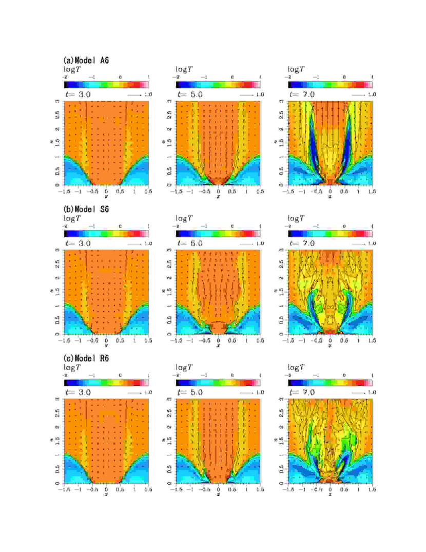
Figure 1: Time evolution of the temperature for a model with $E_{mg}=5.0\times 10^{-4}$ in each perturbation case. Time $t\sim 2\pi\simeq 6.28$ corresponds to one orbital period at $(r,z)=(1,0)$. Lines show the contour of the temperature and arrows show the poloidal velocity.

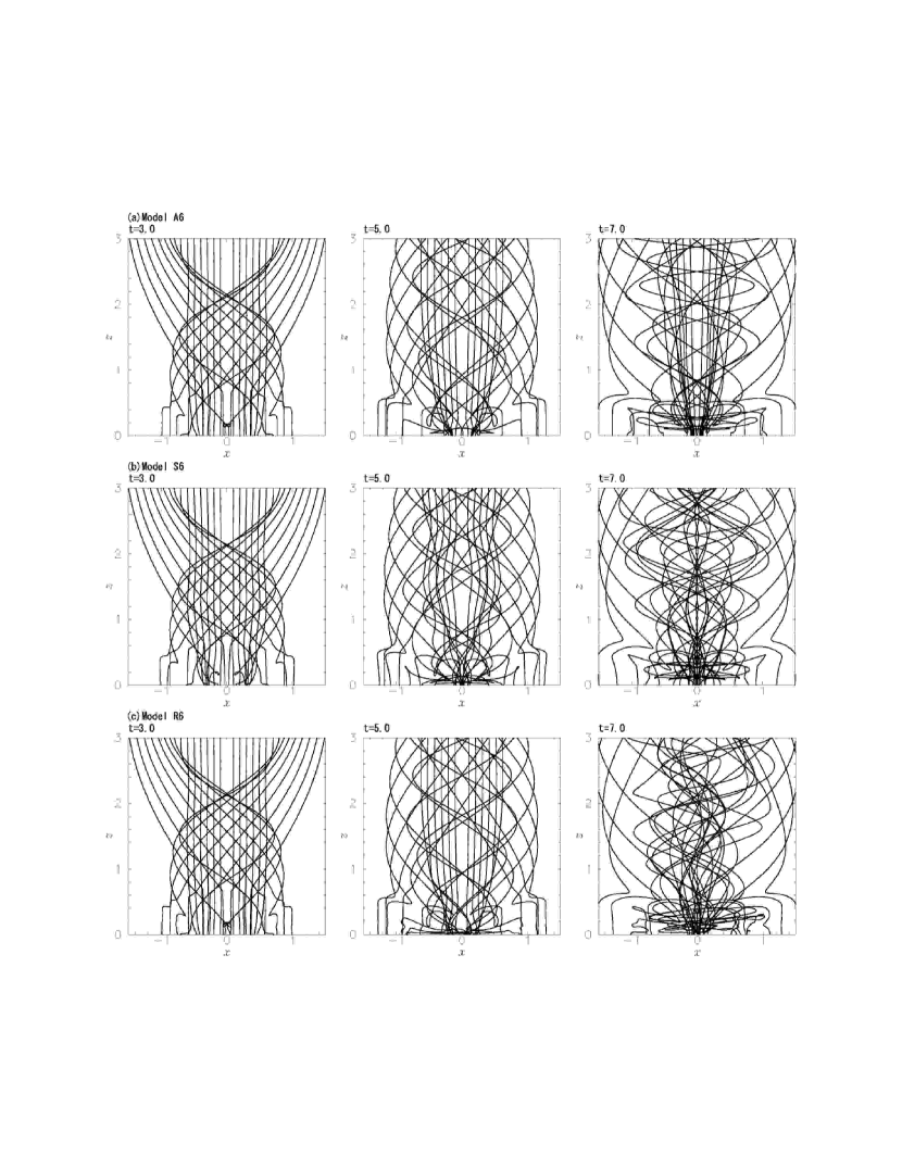
Figure 2: Time evolution of the magnetic field lines projected onto the $x-z$ plane in each perturbation case.

Figure 1 shows the time evolution of the temperature ($T\equiv\gamma p/\rho$; the color and contour) and the poloidal velocity (the arrows) for the typical model ($E_{mg}=5.0\times 10^{-4}$) of each perturbation case. In these cases, the initial values of plasma-$\beta$ ($\equiv 8\pi p/\bm{B}^{2}$) are $\beta\simeq 200$ at $(r,z)=(1,0)$, i.e., at the densest point of the disk, and $\beta\simeq 4$ at $(r,z)=(0,1)$ in the corona. The initial values of plasma-$\beta$ for all models are summarized in Table 2. Time $t=2\pi\simeq 6.28$ corresponds to one Keplerian orbit at $(r,z)=(1,0)$. Figure 2 and 3 show the time evolution of selected magnetic field lines projected onto the $x-z$ and $x-y$ plane.

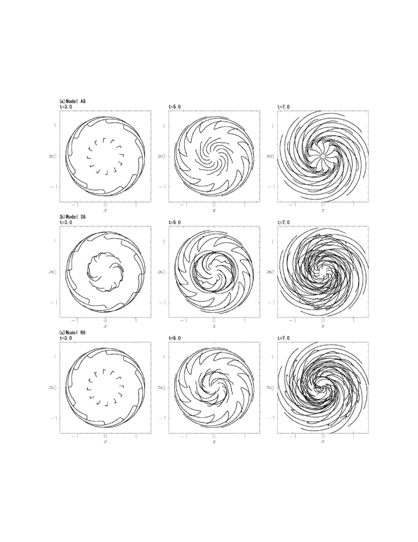
Figure 3: Time evolution of the magnetic field lines projected onto the $r-z$ plane in each perturbation case.

The magnetic field is twisted by the disk rotation and the toroidal field is continuously generated. It propagates into two directions along the large scale magnetic field as a torsional Alfvén wave. Deformed magnetic field brakes the disk rotation. The disk matter loses the angular momentum and falls to the central object while the torsional Alfvén wave transports the angular momentum to the corona. The rotational velocity of the accreted matter increases because the matter falls into the deeper part of the gravitational potential according to the displacement toward the center. It promotes the angular momentum transport by the torsional Alfvén wave propagation. In the sinusoidal perturbation case, the magnetic field is more twisted than in other two cases in the early stage ($t=3.0$; see Figure 3). It indicates more effective extraction of the angular momentum from the accretion disk. The matter on the disk surface layer falls faster than that in the equatorial region in the same way as in Matsumoto et al. (1996) and Kudoh et al. (1998). This is called the avalanche flow.

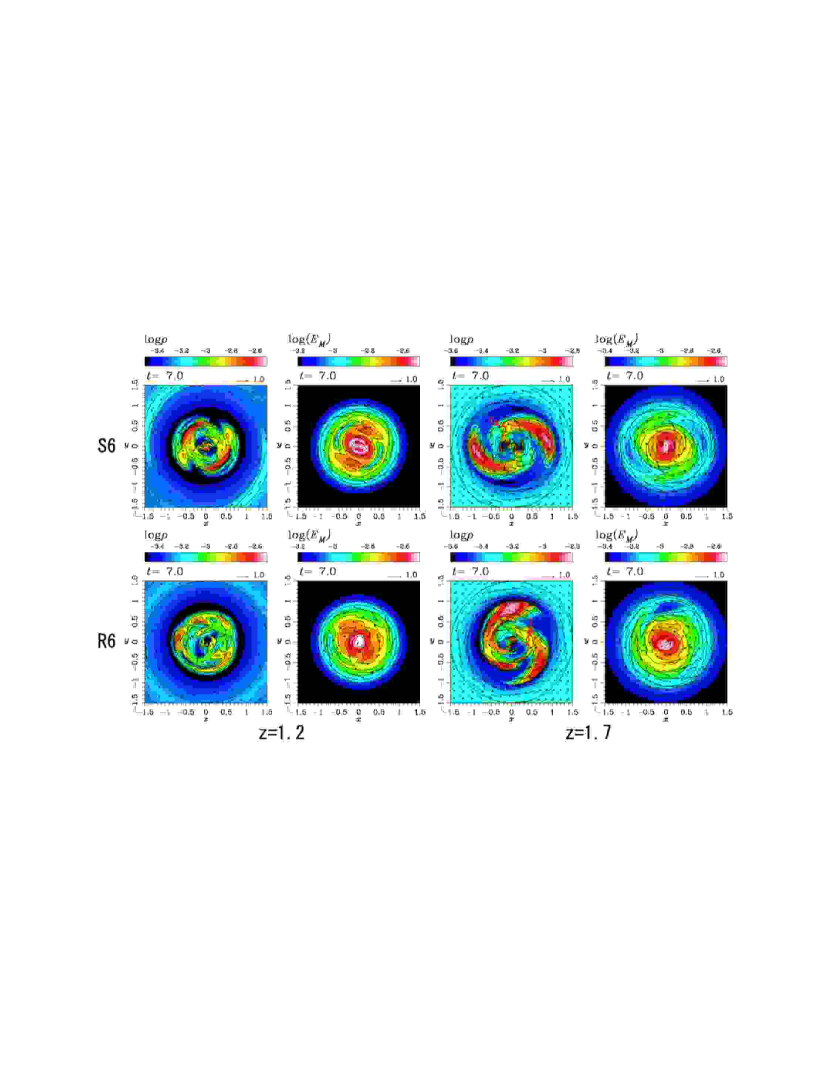
Figure 4: The slice images of the jets on the $z=1.2$ and $1.7$ plane. The upper four figures are the results of the model S6. The lower four figures are the results of the model R6. The color shows the distribution of the density or the magnetic energy and arrows show the velocity field projected onto the plane. There is an anti-correlation between the density and magnetic field distributions. Stability conditions for Kelvin-Helmholtz instability are checked between the point $1$ and $2$ in §4.1.

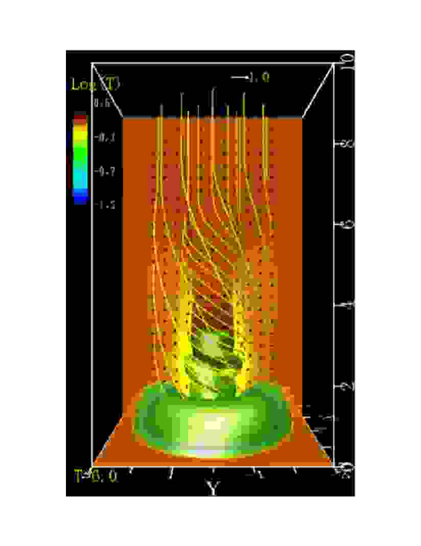
Figure 6: The 3-dimensional visualization of the selected magnetic field lines and the iso-density surface ($\rho=0.0007$) for the model R6 at $t=6.0$. The color shows the distribution of logarithmic temperature and the arrows show the velocity field on the $x=0.0$ plane.

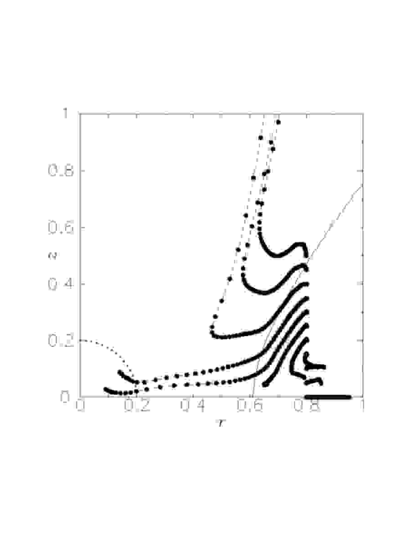
Figure 7: The trajectories of the Lagrangian fluid elements $(0<t<6.1)$ which are initially on a magnetic field line $(r=0.8$ at $t=0)$ in the model A6. The solid line shows the initial disk surface. The dotted line indicates the region where the gravitational potential is softened $(R=(r^{2}+z^{2})^{1/2}<0.2)$. The dashed line shows the trajectory of each element and the filled circles show the Lagrangian fluid elements plotted with time interval of 0.1.

The disk rotation amplifies the magnetic field and the magnetic pressure increases near the equatorial plane. The magnetic pressure gradient force as well as the magnetic centrifugal force accelerates the disk matter in the vertical direction and the jet is formed (see Figure 7d). Just after the ejection of the jet ($t=5.0$), a disk deformation is most remarkable in the sinusoidal perturbation case. It is also apparent that stream lines of outflow show bending pattern in the sinusoidal case although the difference between the axisymmetric case and the random perturbation case is not so notable. At $t=7.0$, the difference between the model A6 and the model R6 also becomes clear. Figure 4 shows the slice images of the jets on the $z=1.2$ and $1.7$ planes at $t=7.0$. The upper four figures are the results of the model S6. The lower four figures are the results of the model R6. The color shows the distribution of the density or the magnetic energy and arrows show the velocity field projected onto the plane. There is an anti-correlation between the density and magnetic field distributions. Stability conditions for Kelvin-Helmholtz instability are checked between the point $1$ and $2$ in §4.1. In the model S6, initial perturbation is of $m=2$ ($m$ is the azimuthal wave number), so that physical variable distributions have the periodicity of $\Delta\phi=\pm\pi$. It is to be noted that the high density regions in Figure 4 are not jets. The high density regions are formed by the compression of the corona matter. This is certified by Figure 5 showing the distribution of $\Theta$ on the $z=1.7$ plane at $t=7.0$. The region where $\Theta=1$ means the place the disk matter exists. Figure 6 is the 3-dimensional visualization of the selected magnetic field lines and the iso-density surface for the model R6 at $t=6.0$. A helical pattern of the density distribution is seen.

3.2 The Lagrangian Fluid Elements along a Field Line

Figure 7 shows the trajectories of the Lagrangian fluid elements $(0<t<6.1)$ which are initially on a magnetic field line $(r=0.8$ at $t=0)$ in the model A6. The elements initially located near the disk surface lose the angular momentum and are accreted toward the central object or ejected as a jet. Those initially located near the equatorial plane remain in the disk.

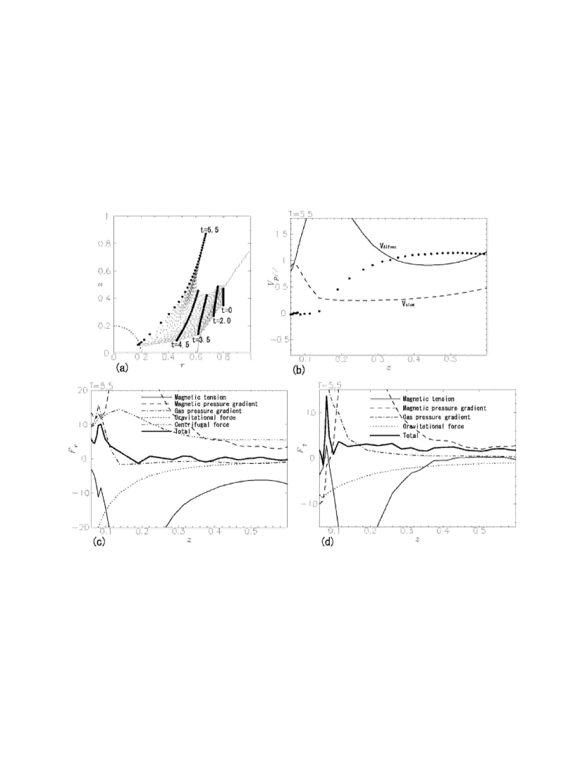
Figure 8: (a)The trajectories of the Lagrangian fluid elements $(0<t<5.5)$ those are initially located near the disk surface and on the same magnetic field line as shown in Figure 7. (b)The poloidal velocity along the magnetic field line $(v_{p\parallel})$ at the each Lagrangian fluid element position at $t=5.5$. The horizontal axis is the position ($z$) of each element and the vertical axis is the velocity. The solid line shows the poloidal Alfvén velocity and the dashed line shows the slow magnetosonic velocity. (c)The $r$-component of each force. (d)The $z$-component of each force. The solid line is the magnetic tension, the dashed line is the magnetic pressure gradient force, the dash-dotted line is the gas pressure gradient force, the dotted line is the gravitational force, the dash-triple-dotted line is the centrifugal force, and the thick solid line is the sum of them.

Figure 8a shows the trajectories of the Lagrangian fluid elements $(0<t<5.5)$ which are initially located near the disk surface and on the same magnetic field line as shown in Figure 7. Figure 8b indicates the poloidal velocity along the magnetic field line $(v_{p\parallel})$ at each Lagrangian fluid element position at $t=5.5$. The horizontal axis is the position ($z$) of each element and the vertical axis is the velocity. The solid line shows the poloidal Alfvén velocity and the dashed line shows the slow magnetosonic velocity. The elements are accelerated to be superslow magnetosonic and trans-Alfvénic. Figure 8c and 8d display the $r$- and $z$-components of each force. The solid line is the magnetic tension, the dashed line is the magnetic pressure gradient force, the dash-dotted line is the gas pressure gradient force, the dotted line is the gravitational force, the dash-triple-dotted line is the centrifugal force, and the thick solid line is the sum of them. The magnetic tension (hoop stress) balances with the magnetic pressure gradient force + centrifugal force, and maintains the collimated flow. The magnetic pressure gradient force and the centrifugal force accelerate the flow in the axial ($z$) and radial ($r$) directions. The gas pressure gradient force tends to zero and becomes inefficient.

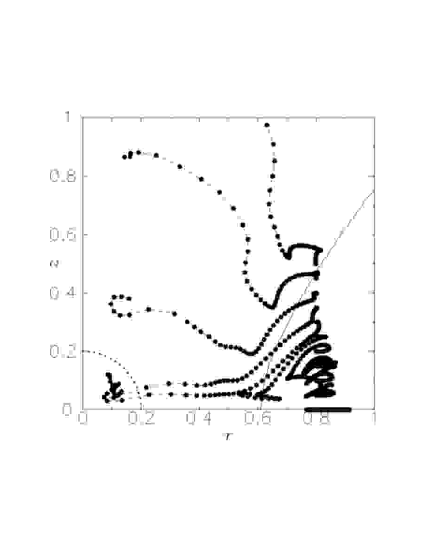
Figure 9: Similar to Fig. 7, but for the model S6. Initial azimuthal position of the Lagrangian fluid elements is 0.

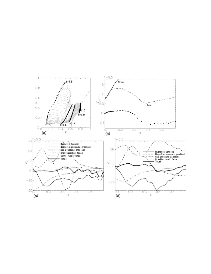
Figure 10: Similar to Fig. 8, but for the model S6. Initial azimuthal position of the Lagrangian fluid elements is 0.

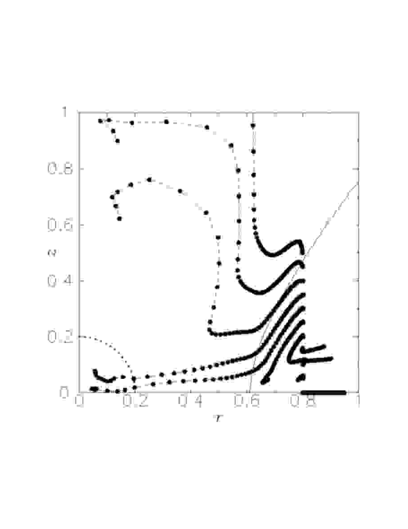
Figure 11: Similar to Fig. 7, but for the model R6. Initial azimuthal position of the Lagrangian fluid elements is 0.

In the non-axisymmetric calculations, the trajectories are different according to the initial azimuthal position of the Lagrangian fluid elements. A part of elements show trajectories similar to those in the axisymmetric calculation, but another part of elements show remarkably different trajectories. Figure 9 is similar to Figure 7, but for the model S6. Initial azimuthal position of the elements is $\phi=0$. Part of elements whose initial $z$ positions are the same as those ejected as a jet in the model A6 move toward the rotational axis of the accretion disk. This is caused because the radial magnetic pressure gradient and centrifugal forces against the magnetic pinch force are smaller than those in the axisymmetric case (see Figure 10c). Figure 10a shows the trajectories of the elements initially located near the disk surface and on the same magnetic field line as shown in Figure 9. A part of the elements are once accelerated in the $z$-direction (after $t=4.5$), but those are forced to go toward the axis. The angle between the poloidal velocity and the poloidal magnetic field is larger than $\pi/2$ (see Figure 10b). Figure 10c and 10d indicate the $r$- and $z$-components of each force. The $r$-components of the magnetic and gas pressure gradient forces show variabilities in the $z$-direction compared to the model A6. The gas pressure gradient force does not tend to zero in both $r$- and $z$-components. The $r$-component of the magnetic tension shows the bending curve. This may be the reason of the bending pattern of the jet (see §3.1 and Figure 1). Figure 11 and 12 are similar to Figure 7 and 8 for the model R6. The reason for a element going toward the rotational axis is the same as for the model S6; that is, the decrease of the radial magnetic pressure gradient and centrifugal forces. Initial azimuthal position of the elements is 0. These figures indicate the characteristics similar to those for the model S6 except the gas pressure gradient force being nearly equal to zero beyond $z\sim 0.45$.

3.3 Dependences on the Initial Magnetic Field Strength

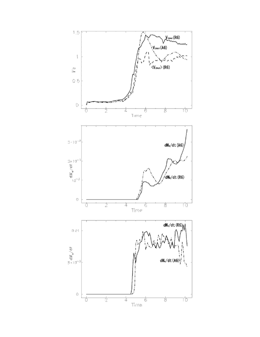
Figure 13: The time variation of the vertical velocity ($v_{z}$), the mass outflow rate, and the mass accretion rate for the model R6 and A6. The mass outflow rate is measured on the $z=1.0$ plane and the mass accretion rate is measured on the $r=0.2$ plane (see §3.3). As for the vertical velocity, the spatially maximum value of $v_{z}$ and azimuthally averaged $v_{z}$ ($\langle v_{z}\rangle$) for the model R6 are plotted.

Kudoh et al. (1998) pointed out that the characteristics of the jet and accretion in nonsteady MHD simulations are similar to those of the steady ones, although the jet and disk in the simulations are essentially nonsteady. (In the resistive cases, Kuwabara et al. (2000) and Casse & Keppens (2002, 2004) showed that the jet and accretion reach the steady state.) How about in the 3-dimensional cases? The jet and accretion in the 3-dimensional cases are also nonsteady. As an example, we show the time variation of the vertical velocity ($v_{z}$), the mass outflow rate, and the mass accretion rate for the model R6 and A6 (Figure 13). As for the vertical velocity, the spatially maximum value of $v_{z}$ and azimuthally averaged $v_{z}$ ($\langle v_{z}\rangle$) for the model R6 are plotted.

To investigate the macroscopic characteristics of the non-axisymmetric MHD jets, the dependences of the maximum jet velocities $(v_{z})$, the maximum mass outflow rates $(\dot{M}_{w}=dM_{w}/dt)$, and the maximum mass accretion rates $(\dot{M}_{a}=dM_{a}/dt)$ on the initial magnetic field strength, $E_{mg}$, are calculated and compared with those in the axisymmetric case. These values are measured only for the material that is initially in the disk by using the function $\Theta$.

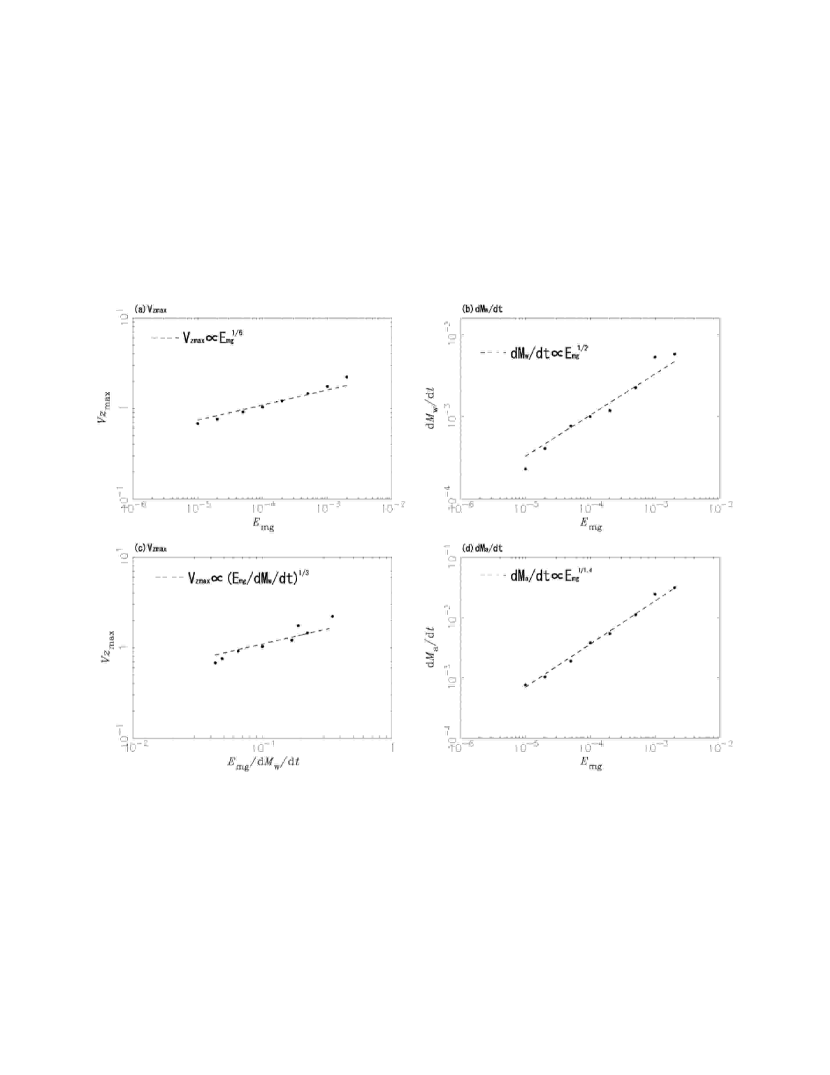
Figure 14: The dependences on the initial magnetic field strength for the random perturbation cases. (a)The maximum velocities of jets as a function of magnetic energy $E_{mg}=V_{A0}^{2}/V_{K0}^{2}$ for the random perturbation cases. The broken line shows $v_{z}\propto E_{mg}^{1/6}$. (b)The maximum mass outflow rates of jets as a function of magnetic energy $E_{mg}=V_{A0}^{2}/V_{K0}^{2}$ for the random perturbation cases. The broken line shows $dM_{w}/dt\propto E_{mg}^{0.5}$. (c)The maximum velocities of jets as a function of $E_{mg}/dM_{w}/dt$ for the random perturbation cases. The broken line shows $v_{z}\propto\left(E_{mg}/dM_{w}/dt\right)^{1/3}$. (d)The maximum mass accretion rates of jets as a function of magnetic energy $E_{mg}=V_{A0}^{2}/V_{K0}^{2}$ for the random perturbation cases. The broken line shows $dM_{a}/dt\propto E_{mg}^{1/1.4}$.

As shown in Kudoh et al. (1998), the maximum jet velocity is proportional to $E_{mg}^{1/6}\propto B_{0}^{1/3}$ and is of the order of the Keplerian velocity. The maximum jet velocities in both sinusoidal and random perturbation cases have the same dependence as that in the axisymmetric case and are also of the order of the Keplerian velocity. As an example, the maximum jet velocities as a function of $E_{mg}$ in the random perturbation case are shown in Figure 14a. The broken line shows $v_{z}\propto E_{mg}^{1/6}\propto B_{0}^{1/3}$.

The definition of the mass outflow rate $(\dot{M}_{w})$ of the jet is

$$\dot{M}_{w}=\int_{0}^{2\pi}\int_{0}^{1}\rho v_{z}rdrd\phi\\$$ (22)

at $z=1$. Kudoh et al. (1998) showed that $\dot{M}_{w}$ is proportional to $E_{mg}^{0.5}\propto B_{0}$. The maximum mass outflow rates in both perturbation cases also have the same dependence on $E_{mg}$ as that in the axisymmetric case. Figure 14b shows the maximum mass outflow rates as a function of $E_{mg}$ in the random perturbation case. The broken line shows $\dot{M}_{w}\propto E_{mg}^{0.5}\propto B_{0}$.

As mentioned in Kudoh et al. (1998), these two relations are interpreted as the Michel’s solution, $v_{\infty}\propto(B_{0}^{2}/\dot{M}_{w})^{1/3}$, in the magnetic pressure driven jet regime ($\dot{M}_{w}\propto E_{mg}^{0.5}\propto B_{0}$). Figure 14c shows the maximum jet velocities as a function of $E_{mg}/\dot{M}_{w}$ in the random perturbation case. The broken line shows $v_{z}\propto(E_{mg}/\dot{M}_{w})^{1/3}$. The maximum jet velocities in our simulations are approximately proportional to $(E_{mg}/\dot{M}_{w})^{1/3}$. This result indicates that the MHD jets even in the 3-dimension are consistent with the Michel’s steady solution, even before the jets reaching the steady state.

The mass accretion rate $(\dot{M}_{a})$ is defined by

$$\dot{M}_{a}=-\int_{0}^{2\pi}\int_{0}^{1}\rho v_{r}rd\phi dz$$ (23)

at $r=0.2$. Figure 14d shows the maximum mass accretion rates as a function of $E_{mg}$ in the random perturbation case. The broken line shows $\dot{M}_{a}\propto E_{mg}^{1/1.4}$. $\dot{M}_{a}$ is well fitted by $\dot{M}_{a}\propto E_{mg}^{1/1.4}\sim E_{mg}^{0.7}\propto B_{0}^{1.4}$ as same as in the axisymmetric case shown in Kudoh et al. (1998). $\dot{M}_{a}$ in the sinusoidal perturbation case also has the same dependence on $E_{mg}$.

4 Discussion

4.1 Non-axisymmetric Structure in the Jets

Lobanov & Zensus (2001) found that the 3C273 jet has a double helical structure and that it can be fitted by two surface modes and three body modes of Kelvin-Helmholtz (K-H) instability. On the other hand, the jet launched from the disk in our simulation has a non-axisymmetric ($m=2$) structure in both perturbation cases (see Figure 4).

The stability condition for non-axisymmetric K-H surface modes is

$$\Delta V<V_{As}=\left[\frac{\rho_{1}+\rho_{2}}{4\pi\rho_{1}\rho_{2}}\left({\bm{B}_{1}}^{2}+{\bm{B}_{2}}^{2}\right)\right]^{1/2}$$ (24)

where $\Delta V\equiv V_{1}-V_{2}$ and $V_{As}$ is called as a “surface” Alfvén velocity (Hardee & Rosen 2002). Figure 4 shows the distribution of logarithmic density on the $z=1.7$ plane at $t=7.0$ for the model S6 and R6. We check the above-mentioned stability condition between the point $1$ and $2$. In the model S6, $\Delta V_{12}=0.38$ (in this case, $\Delta V$ is a difference of $v_{z}$) and $V_{As12}=16$. In the model R6, $\Delta V_{12}=0.29$ and $V_{As12}=16$. Therefore, the non-axisymmetric structure in the jets is not produced by K-H surface modes.

Non-axisymmetric K-H body modes become unstable if jet velocity is super-fast magnetosonic ($V_{FM}<V_{j}$) or is slightly below the slow magnetosonic velocity ($C_{s}V_{A}/(C_{s}^{2}+V_{A}^{2})^{1/2}<V_{j}<V_{SM}$) (Hardee & Rosen 1999), where $C_{s}$ is the sound velocity and $V_{A}$ is the Alfvén velocity. The jets in the model S6 and R6 satisfy the former unstable condition for a little time, but after the short time unstable phase the jets become stable for that condition. It can be said that body modes of K-H instability can not explain the production of the non-axisymmetric structure.

As for the velocity field, the observational results indicating the rotation of YSO jets have recently been obtained (e.g., Bacciotti et al. 2002; Coffey et al. 2004). In our simulations, the jets have the non-axisymmetric helical velocity field (see $v_{zmax}$ and $\langle v_{zmax}\rangle$ in Figure 13). Such velocity field may be observed in the future.

4.2 Connection of Non-axisymmetric Structure between Disk and Jet

To investigate a connection of the non-axisymmetric structure in the jet and that in the disk, we calculate the Fourier power spectra of the non-axisymmetric modes of the magnetic energy in the disk or in the jet.

$$\tilde{E}_{M}\left(k_{r},m,k_{z}\right)=\frac{1}{V_{s}}\int\!\!\!\int\!\!\!\int_{V_{s}}E_{M}\left(r,\phi,z\right)e^{i\left(k_{r}r+m\phi+k_{z}z\right)}rdrd\phi dz$$ (25)

where $E_{M}$ is the magnetic energy $(\bm{B}^{2}/8\pi)$. $V_{s}$ means the volume of the disk or the jet. To concentrate on non-axisymmetric modes, $\tilde{E}_{M}$ is integrated about the radial and axial wave number ($k_{r}$ and $k_{z}$). The definition of the disk or the jet is the following:

• The disk is the region where the function $\Theta$ is not equal to 0 and $z\leq$ 1.5.

• The jet is the region where the function $\Theta$ is not equal to 0 and $z>$ 1.5.

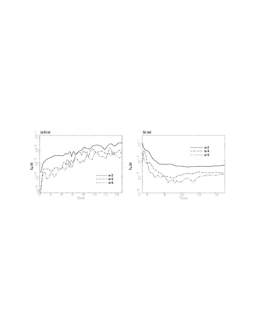
Figure 15: Time evolution of Fourier power spectra of the magnetic energy in the model S6. (a)In the disk and (b)in the jet.

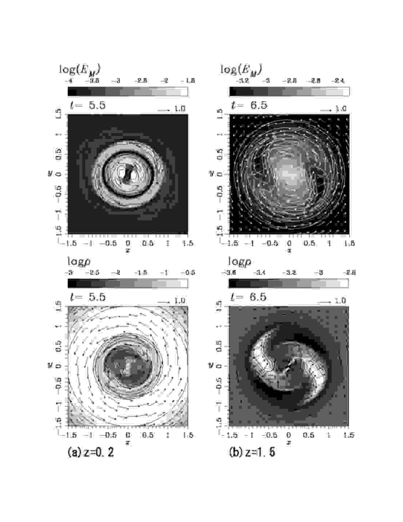
Figure 16: The distribution of the magnetic energy and the logarithmic density (a)on the $z=0.2$ plane (in the disk) at $t=5.5$ and (b)on the $z=1.5$ plane (in the jet) at $t=6.5$ in the model S6.

Figure 15 shows the time evolution of Fourier power spectra of the magnetic energy in the model S6. In the cases of the disk with sinusoidal perturbation ($\delta v_{\phi}\propto\sin 2\phi$), the calculations have the periodicity of $\Delta\phi=\pm\pi$, so that we calculate the power spectra with even azimuthal wave number. The $m=2$ mode is dominant from the first stage of the run in the disk (see Figure 15a) because the initial perturbation is of pure $m=2$ mode. The $m=2$ mode spectrum becomes almost constant level, and then increases continuously with oscillation. The $m=4$ and $6$ modes also start to grow at almost the same time with the $m=2$ mode. Their growth is also with oscillation and with almost the same growth rate. Fourier power spectra of the magnetic energy in the jet (see Figure 15b) are not calculated before $t=5.4$ because the jet is not launched before that. The $m=2$ mode is dominant in the jet as well as in the disk. The power spectra of all the non-axisymmetric modes become nearly constant with time in the jet. The each mode spectrum in the jet is not with oscillation by contrast with the growth of each mode in the disk. Figure 16 shows the distribution of the magnetic energy and the logarithmic density on the $z=0.2$ plane (in the disk) at $t=5.5$ and on the $z=1.5$ plane (in the jet) at $t=6.5$. The non-axisymmetric structure with $m=2$ is clearly seen.

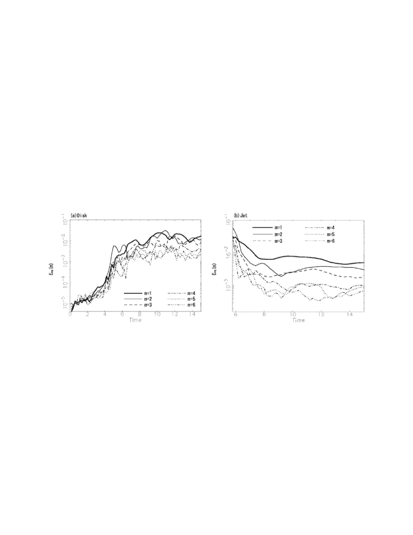
Figure 17: Similar to Fig. 15, but for the model R6.

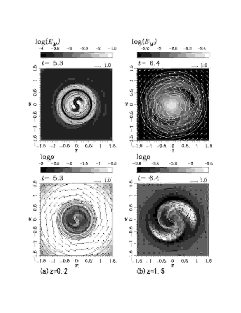
Figure 18: The distribution of the magnetic energy and the logarithmic density (a)on the $z=0.2$ plane (in the disk) at $t=5.3$ and (b)on the $z=1.5$ plane (in the jet) at $t=6.4$ in the model R6.

Figure 17 shows the Fourier power spectra of the magnetic energy in the model R6 as functions of time. In this case the initial perturbation has no particular mode, so that all modes show the growth with almost the same growth rate in the first stage in the disk (see Figure 17a). The $m=2$ mode becomes dominant around $t=5.0$ in the disk. The $m=2$ mode spectrum, however, decreases for a time. At the same time, the growth rates of other modes also decrease. These can be thought to be related to the jet ejection. After the jet ejection, the $m=2$ mode becomes comparable to or predominant over the $m=1$ mode though, roughly speaking, the Fourier power spectrum is larger the longer (the smaller) the azimuthal wave length (wave number) is. As same as in the model S6, the growth of each mode in the disk shows oscillation though it can not be seen in the jet. It can be thought that the oscillation in the disk is related to the mass accretion (see also the bottom panel of Figure 13). The $m=2$ mode is initially dominant in the jet, which is probably connected to the peak in the disk at $t=5.0$. In response to the decrease of the $m=2$ mode spectrum in the disk, that in the jet also decreases. However the $m=2$ mode spectrum becomes comparable to the $m=1$ mode spectrum later. It is to be noted that the power spectra of all the non-axisymmetric modes become nearly constant with time in the jet as well as in the case of the sinusoidally perturbed disk. Figure 18 shows the distribution of the magnetic energy and the logarithmic density on the $z=0.2$ plane (in the disk) at $t=5.3$ and on the $z=1.5$ plane (in the jet) at $t=6.4$.

4.3 Origin of the Non-axisymmetric Structure

What mechanism makes the non-axisymmetric structure? In the previous section, it is made clear that the non-axisymmetric structure in the jet originates in the accretion disk. In this section, we discuss the cause of the non-axisymmetric structure in the disk. At first, the possibility of the magnetorotational instability (MRI; Balbus & Hawley 1991) is examined. The dispersion relation for the non-axisymmetric disturbance was given by Balbus & Hawley (1992) (see the equation 2.24 in that paper). The dispersion relation equation is numerically solved; from the simulation result (e.g., Figure 18a) $\lambda_{r}=0.4$. The radial coordinate, $R$ in the equation, is assumed to be 1.0, where the avalanche-like accretion flow is initially remarkably formed. The axial wave length $\lambda_{z}$ is assumed to be 0.35, which is almost equal to the most unstable wavelength, $\lambda\sim 2\pi V_{A}/\Omega$. From the initial condition, $\bm{V}_{A}=(V_{Ar},V_{A\phi},V_{Az})=(0,0,0.056)$ and $\Omega=1.0$ at $r=1.0$. The epicyclic frequency $\kappa$ is zero because of the constant angular momentum disk. The azimuthal wave number $m$ is the parameter.

One of the four roots is the unstable solution in all the ($m$=1$\sim$6) cases. The growth rate is higher the smaller the azimuthal wave number $m$ is, although the $m=2$ growth rate is comparable to the $m=1$ growth rate. The calculated growth rate, $\omega$, of the $m=2$ mode is about 0.54, and $\rm{exp}\left(\omega t\right)$ at $t=3.0$ is 5.1. The numerical result shows the increase of the $m=2$ mode spectrum by a factor of 5.9. These are consistent with the initial evolution of the modes in the disk (see Figure 17a). After about $t=3.0$, the mode spectra show the non-linear growth. The temporal dominance of $m=2$ mode in the disk in the model R6 is at the MRI non-linear growth stage.

We briefly comment on the possibility of other instabilities. As showed in §4.1, the K-H instabilities are stable between the jet and the ambient gas. How about between the accretion disk and the corona? In our simulations, they seem to be stable or the growth rates seem to be small because no growth of the K-H instabilities is seen in the hydrodynamic (no magnetic field) simulation. Another probable instability is a magnetic analogue of the non-axisymmetric hydrodynamical instability in the constant angular momentum torus, so-called Papaloizou-Pringle instability (Papaloizou & Pringle 1984; Goldreich, Goodman, & Narayan 1986; Hawley 1990). Curry & Pudritz (1996) investigated the growth rate of the instability in various conditions. According to their result, the (magnetic) PP instability seems not to make an important contribution for forming the non-axisymmetric structure. The magnetic field is relatively weak (normalized Alfvén velocity, $V_{z}$ in Curry & Pudritz, is equal to 0.056) so that it is almost hydrodynamic. Indeed, the plasma-$\beta$ in the disk is of the order of a hundred. In such case, the growth rate is small.

4.4 Amplification of Magnetic Field in the Disk

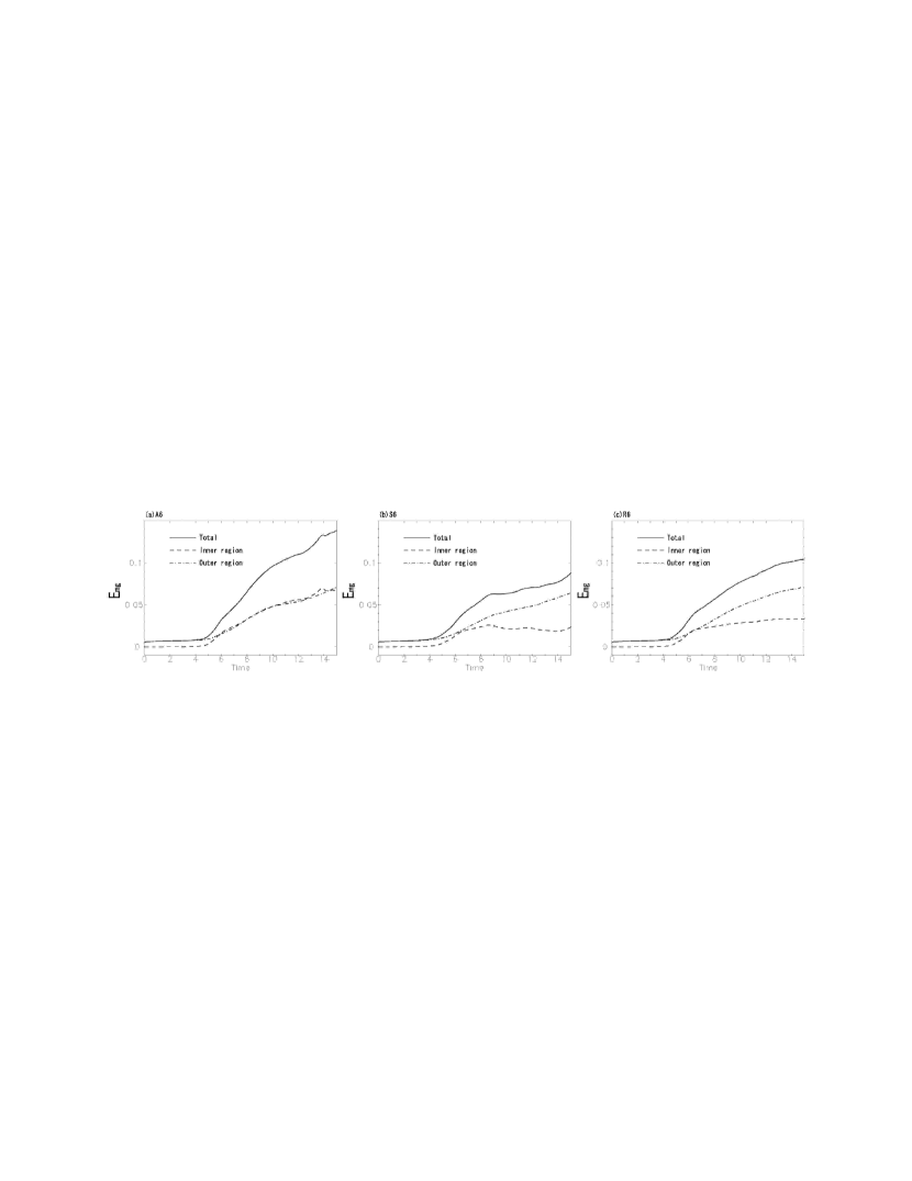
Figure 19: Time evolution of the space-integrated magnetic energy in the accretion disk in each perturbation case. The solid line shows the magnetic energy in all the region of the disk. The broken or dash-dotted line shows the magnetic energy only in the inner ($r\leq 0.6$) or outer ($r>0.6$) region of the disk respectively.

Differentially rotating disks with a magnetic field amplify its magnetic field by the MRI. In this section we investigate the difference of the amplification depending on the form of the perturbation. Figure 19 shows the time variation of the magnetic energy in the disk. The definition of the disk is the same as that in the previous section. The solid line is the magnetic energy in all the region of the disk ($\int\bm{B}^{2}/8\pi\ dV_{disk}$), where $V_{disk}$ is the volume of the disk. The broken line is the magnetic energy only in the inner region ($r\leq 0.6$) of the disk and the dash-dotted line is the magnetic energy only in the outer region ($r>0.6$) of the disk. The magnetic energy in the disk is most amplified in the axisymmetric case. The magnetic energy in the inner region displays a striking difference between the axisymmetric case and the other two cases though the magnetic energy in the outer region is almost the same. The total magnetic energy at $t=15.0$, therefore, shows the difference. The differences from the value for the model A6 are -0.051 and -0.034 for the model S6 and R6 respectively.

The time variation of the magnetic energy is described by the following equation.

$$\frac{\partial}{\partial t}\left(\frac{\bm{B}^{2}}{8\pi}\right)=-\bm{v}\cdot\left(\bm{J}\times\bm{B}\right)-\frac{1}{4\pi}\nabla\cdot\left(\bm{E}\times\bm{B}\right)$$ (26)

where $\bm{J}=\left(\nabla\times\bm{B}\right)/4\pi$. The first term in the right hand means the conversion of magnetic energy to kinetic energy by the Lorentz force. The second term is the transportation of the energy by Poynting flux. It is investigated below that a difference of the value of the first or second term in the equation (26) can explain the difference of the magnetic energy.

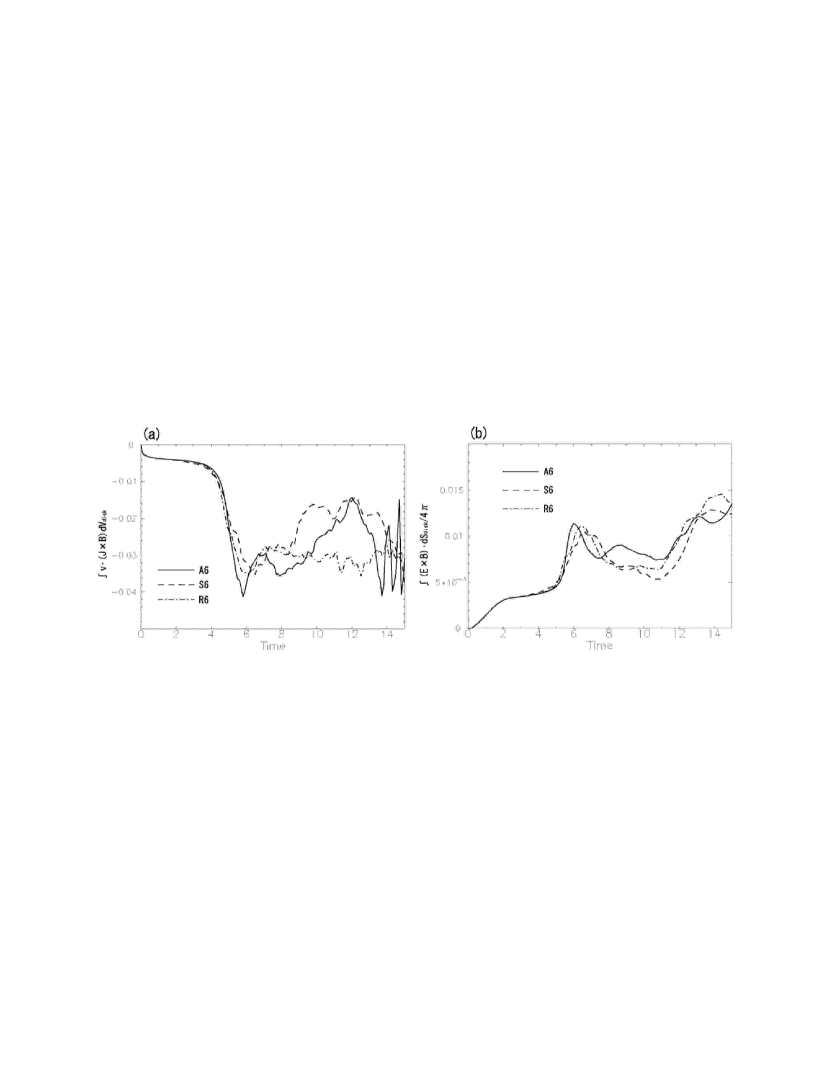
Figure 20: (a)Time evolution of the work done by the Lorentz force in the accretion disk. A negative value means kinetic energy is converted to magnetic energy. (b)Time evolution of Poynting energy flowing out through a “disk surface” (see the text as regards the detailed definition of the “disk surface”).

Figure 20a shows the work done by the Lorentz force in the disk ($\int\bm{v}\cdot\left(\bm{J}\times\bm{B}\right)dV_{disk}$; a negative value means kinetic energy is converted to magnetic energy). The time integration of the work done by Lorentz force between $t=0.0$ and $t=15.0$ is done to investigate the origin of the difference in the magnetic energy between the different models, A6, S6, and R6. For discussing the amplification of the magnetic energy, the sign should be inverted. The results are 0.32, 0.26, and 0.34 for the model A6, S6, and R6 respectively. The differences from the value for the model A6 are -0.051 and 0.022 for the model S6 and R6 respectively.

The another term is the energy transportation by Poynting flux. To calculate this value, the vector normal to the disk surface must be determined. However that is difficult, so that, for simplicity, the “disk surface” is defined as the $z=1.5$ plane ($r\leq 2.0$) and the $r=2.0$ plane ($z\leq 1.5$). Figure 20b shows the value of $\int\left(\bm{E}\times\bm{B}\right)/4\pi\ dS_{disk}$ as functions of time for the model A6 (solid line), S6 (broken line), and R6 (dash-dotted line). The results of the time integral of this value between $t=0.0$ and $t=15.0$ are -0.11, -0.10, and -0.11 for the model A6, S6, and R6 respectively (the sign is inverted for discussing the amplification of the magnetic energy). The differences from the value for the model A6 are 0.01 (S6) and 0.0 (R6).

As regards the model S6, the difference of the magnetic energy from that for the model A6 at $t=15.0$ can be explained by the difference of the work done by the Lorentz force, ignoring the contribution of Poynting flux. On the other hand, the magnetic energy for the model R6 should become larger than that for the model A6 by 0.022. The magnetic energy for the model R6 at $t=15.0$ is, however, smaller than that for the model A6 by 0.034. It means that the magnetic energy is dissipated by 0.056. The dissipation takes place at the inner region $(r\leq 0.6)$ of the disk (see Figure 19). One possibility is the numerical magnetic reconnection. To confirm this point, resistive MHD simulations are necessary. It is to be noted that the magnetic reconnection in the innermost region of the accretion disk is proposed to be the origin of X-ray shots observed in black hole candidates (Machida & Matsumoto 2003). In any case, the physical process at the inner region of the disk seems to be important.

4.5 Parameters in the Disk for Each Case

Table 3, 4, and 5 summarize several physical values calculated from the simulation result of the axisymmetric, the sinusoidal perturbation, and the random perturbation case respectively. The second column shows the initial space-averaged magnetic energy in the disk. The space-average of a certain physical quantity, $f$, is calculated as follows: $\langle f\rangle=\int_{V_{s}}fdV/V_{s}$, where $V_{s}$ is the volume of the disk. The definition of the disk is the same as in §4.2. The third one shows the maximum space-averaged magnetic energy in the disk. The fourth one indicates the maximum amplification rate of the magnetic energy in the disk. The runs with the sinusoidal perturbation display the smallest amplification rates in all the magnetic field strength cases compared with the other two perturbation models. This is explained by the fact that in the sinusoidal perturbation case the work done by the Lorentz force is the smallest (see section 4.4). The rate for the random perturbation case is comparable to that for the axisymmetric case when the initial magnetic field strength is relatively small; however the rate for the random perturbation case becomes clearly smaller than that for the axisymmetric case as the initial magnetic field becomes strong. This may be because the magnetic energy dissipates by the numerical magnetic reconnection as discussed in section 4.4.

The fifth column shows the time-averaged ratio of the $r\phi$-component of the space-averaged Maxwell stress to the space-averaged pressure. This value corresponds to the non-dimensional viscous parameter (so-called $\alpha$ parameter). The $\alpha$ parameter means the efficiency of the angular momentum transport. In all the three (axisymmetric, sinusoidal perturbation, or random perturbation) cases, this parameter $(\equiv\alpha_{B,\phi R})$ increases with increasing the initial magnetic field strength. This is equivalent to the fact that the mass accretion rate increases with increasing the initial magnetic field. The sixth column is the time-averaged ratio of the ${\phi}z$-component of the space-averaged Maxwell stress to the space-averaged pressure. This value represents the efficiency of the angular momentum transport in the vertical direction. When we denote $\alpha_{B,\phi R}\propto E_{mg}^{b}$, we find $b$ is $0.66\sim 0.75$; on the other hand $b$ becomes $0.49\sim 0.54$ when $\alpha_{B,\phi Z}$ is fitted. However, $\alpha_{B,\phi R}$ and $\alpha_{B,\phi Z}$ are comparable in the wide range of initial magnetic field strength. The last column shows the space- and time-averaged plasma-$\beta$ in the disk.

Finally we comment on the fact that the dynamical time of our simulations is about 2 orbital periods (strictly speaking, the dynamical time ranges from one a bit smaller than 2 orbital periods to about 2.5 orbital periods, depending on the initial magnetic field strength). In our simulations, the numerical instability often occurred at around 2 rotations of the inner part of the disk by the violently deformed magnetic field . It has often been said that the jets in nonsteady MHD simulations are transient phenomena owing to the particular choice of the initial conditions. However, Ibrahim, Sato, & Shibata (2004), K. Sato et al. (in preparation), and A. Ibrahim et al. (in preparation) performed long-term simulations of MHD jet though the parameters of the accretion disk are different from the parameters in this paper. They showed that time-averages of the jet velocity, mass outflow rate, and mass accretion rate reproduce the scaling law found in Kudoh et al. (1998) although the jets are nonsteady and intermittent. These facts indicate the significance of our results regardless of the short calculation time. It is, of course, interesting whether the instabilities in the jet itself (e.g., the kink and/or K-H instabilities) develop after a long-time evolution. This is an important future work.

5 Conclusions

We performed 3-dimensional MHD simulations of jet formation by solving the accretion disk self-consistently. The accretion disk is perturbed with the non-axisymmetric sinusoidal or random fluctuation of the rotational velocity to investigate the stability of MHD jet ejected from the disk in 3-dimension. Our results are summarized as follows:

1. The jet launched from the accretion disk whose rotational velocity is non-axisymmetrically perturbed has the properties that the jet velocity is proportional to $B_{0}^{1/3}$ and that the mass outflow rate is proportional to $B_{0}$, where $B_{0}$ is the initial magnetic field strength. The dependence of the mass accretion rate ($\dot{M}_{a}$) on the initial magnetic field strength is given by $\dot{M}_{a}\propto B_{0}^{1.4}$. The first relation is consistent with the scaling law of the Michel’s solution (Michel 1969) and the result of the axisymmetric simulation (Kudoh et al. 1998). The other two relations are also consistent with Kudoh et al. (1998). Part of fluid elements, however, show the trajectories remarkably different from those in the axisymmetric case. This is caused by the decrease in the magnetic pressure gradient and centrifugal force in the radial direction those are against the magnetic tension (hoop stress).

2. The jet in both perturbation cases shows the non-axisymmetric structure with $m=2$, where $m$ means the azimuthal wave number. As the origin of the non-axisymmetric structure, the K-H instability is ruled out according to the stability condition. Calculation of the Fourier power spectra of the magnetic energy shows that the $m=2$ mode becomes dominant in the jet at least once. The time evolution of the power spectra indicates that the non-axisymmetric structure in the jet originates in the accretion disk, not in the jet itself. In both perturbation cases, all the non-axisymmetric modes in the jet reach almost constant levels after about 1.5 orbital periods of the accretion disk, while all modes in the accretion disk grow with oscillation.

3. The magnetic energy is amplified in the accretion disk by the magnetorotational instability (MRI). In the non-axisymmetric cases, amplification rates are smaller than that in the axisymmetric case. The difference between the axisymmetric case and the non-axisymmetric cases is notable in the inner region of the accretion disk. In the sinusoidal perturbation case, this is explained by the difference of the work done by the Lorentz force. In the random perturbation case, however, that can not be explained by such difference or the difference of the energy transportation by Poynting flux. One possibility is the numerical reconnection in the inner region of the accretion disk.

4. The space- and time-averaged ratio of the Maxwell stress component that is related to the angular momentum transport in the radial direction to gas pressure, $\langle\langle-B_{r}B_{\phi}/4\pi\rangle/\langle p\rangle\rangle\equiv\alpha_{B,\phi R}$, shows the dependence on the initial magnetic field strength like $\alpha_{B,\phi R}\propto B_{0}^{1.4}$. That for the Maxwell stress component that is related to the angular momentum transport in the vertical direction shows the dependence like $\langle\langle-B_{\phi}B_{z}/4\pi\rangle/\langle p\rangle\rangle\equiv\alpha_{B,\phi Z}\propto B_{0}^{1.0}$. However, $\alpha_{B,\phi Z}$ is comparable to $\alpha_{B,\phi R}$ in the wide range of the initial magnetic field strength.

This work is partly supported by the Japan Society for the Promotion of Science Japan-UK Cooperation Science Program (principal investigators: K. Shibata and N. O. Weiss), and the Grant-in-Aid for the 21st Century COE ”Center for Diversity and Universality in Physics” from the Ministry of Education, Culture, Sports, Science and Technology (MEXT) of Japan. Numerical computations were carried out on VPP5000 at the Astronomical Data Analysis Center of the National Astronomical Observatory, Japan (project ID: yhk32b and rhk05b), which is an interuniversity research institute of astronomy operated by the Ministry of Education, Culture, Sports, Science, and Technology.

Table 1: Normalization Units

Physical Quantities	Description	Normalization Unit
$t$	Time	$r_{0}/V_{K0}$
$r,z$	Length	$r_{0}$
$\rho$	Density	$\rho_{0}$
$p$	Pressure	$\rho_{0}V_{K0}^{2}$
$\bm{v}$	Velocity	$V_{K0}$
$\bm{B}$	Magnetic field	$(\rho_{0}V_{K0}^{2})^{1/2}$

Table 2: Models and Parameters

			Perturbation
$E_{mg}$	$\beta_{0d}$	$\beta_{0c}$	None	Sinusoidal	Random
$1.0\times 10^{-5}$	10200	200	A1	S1	R1
$2.0\times 10^{-5}$	5100	100	A2	S2	R2
$5.0\times 10^{-5}$	2040	40	A3	S3	R3
$1.0\times 10^{-4}$	1020	20	A4	S4	R4
$2.0\times 10^{-4}$	510	10	A5	S5	R5
$5.0\times 10^{-4}$	204	4	A6	S6	R6
$1.0\times 10^{-3}$	102	2	A7	S7	R7
$2.0\times 10^{-3}$	51	1	A8	S8	R8

Table 3: Axisymmetric Runs

Model	$\langle E_{Md0}\rangle$	$\langle E_{Md_{max}}\rangle$	$\left((3)-(2)\right)/(2)$	$\langle\langle-\frac{B_{r}B_{\phi}}{4\pi}\rangle/\langle p\rangle\rangle$	$\langle\langle-\frac{B_{\phi}B_{z}}{4\pi}\rangle/\langle p\rangle\rangle$	$\langle\langle\beta_{d}\rangle\rangle$
(1)	(2)	(3)	(4)	(5)	(6)	(7)
A1	$5.0\times 10^{-6}$	$1.6\times 10^{-4}$	31	0.0035	0.0068	$1.4\times 10^{2}$
A2	$1.0\times 10^{-5}$	$3.3\times 10^{-4}$	32	0.0079	0.012	84
A3	$2.5\times 10^{-5}$	$6.0\times 10^{-4}$	23	0.018	0.022	41
A4	$5.0\times 10^{-5}$	$1.0\times 10^{-3}$	19	0.030	0.032	23
A5	$1.0\times 10^{-4}$	$1.7\times 10^{-3}$	16	0.051	0.044	13
A6	$2.5\times 10^{-4}$	$3.2\times 10^{-3}$	12	0.089	0.063	6.2
A7	$5.0\times 10^{-4}$	$5.7\times 10^{-3}$	10	0.14	0.082	3.4
A8	$1.0\times 10^{-3}$	$7.7\times 10^{-3}$	6.7	0.17	0.093	2.0

Table 4: Sinusoidal Perturbation Runs

Model	$\langle E_{Md0}\rangle$	$\langle E_{Md_{max}}\rangle$	$\left((3)-(2)\right)/(2)$	$\langle\langle-\frac{B_{r}B_{\phi}}{4\pi}\rangle/\langle p\rangle\rangle$	$\langle\langle-\frac{B_{\phi}B_{z}}{4\pi}\rangle/\langle p\rangle\rangle$	$\langle\langle\beta_{d}\rangle\rangle$
(1)	(2)	(3)	(4)	(5)	(6)	(7)
S1	$5.0\times 10^{-6}$	$1.2\times 10^{-4}$	22	0.0027	0.0061	$1.4\times 10^{2}$
S2	$1.0\times 10^{-5}$	$2.1\times 10^{-4}$	20	0.0061	0.011	87
S3	$2.5\times 10^{-5}$	$4.5\times 10^{-4}$	17	0.014	0.021	44
S4	$5.0\times 10^{-5}$	$7.1\times 10^{-4}$	13	0.024	0.032	26
S5	$1.0\times 10^{-4}$	$1.1\times 10^{-3}$	9.5	0.041	0.047	14
S6	$2.5\times 10^{-4}$	$2.0\times 10^{-3}$	7.0	0.073	0.066	6.7
S7	$5.0\times 10^{-4}$	$3.4\times 10^{-3}$	5.8	0.11	0.083	3.8
S8	$1.0\times 10^{-3}$	$4.7\times 10^{-3}$	3.7	0.15	0.10	2.2

Table 5: Random Perturbation Runs

Model	$\langle E_{Md0}\rangle$	$\langle E_{Md_{max}}\rangle$	$\left((3)-(2)\right)/(2)$	$\langle\langle-\frac{B_{r}B_{\phi}}{4\pi}\rangle/\langle p\rangle\rangle$	$\langle\langle-\frac{B_{\phi}B_{z}}{4\pi}\rangle/\langle p\rangle\rangle$	$\langle\langle\beta_{d}\rangle\rangle$
(1)	(2)	(3)	(4)	(5)	(6)	(7)
R1	$5.0\times 10^{-6}$	$1.7\times 10^{-4}$	33	0.0041	0.0056	$1.5\times 10^{2}$
R2	$1.0\times 10^{-5}$	$3.4\times 10^{-4}$	33	0.0090	0.010	88
R3	$2.5\times 10^{-5}$	$7.1\times 10^{-4}$	27	0.021	0.020	44
R4	$5.0\times 10^{-5}$	$9.8\times 10^{-4}$	19	0.033	0.031	26
R5	$1.0\times 10^{-4}$	$1.4\times 10^{-3}$	13	0.048	0.045	15
R6	$2.5\times 10^{-4}$	$2.6\times 10^{-3}$	9.3	0.079	0.067	6.9
R7	$5.0\times 10^{-4}$	$3.9\times 10^{-3}$	6.9	0.12	0.084	3.9
R8	$1.0\times 10^{-3}$	$5.6\times 10^{-3}$	4.6	0.14	0.10	2.3

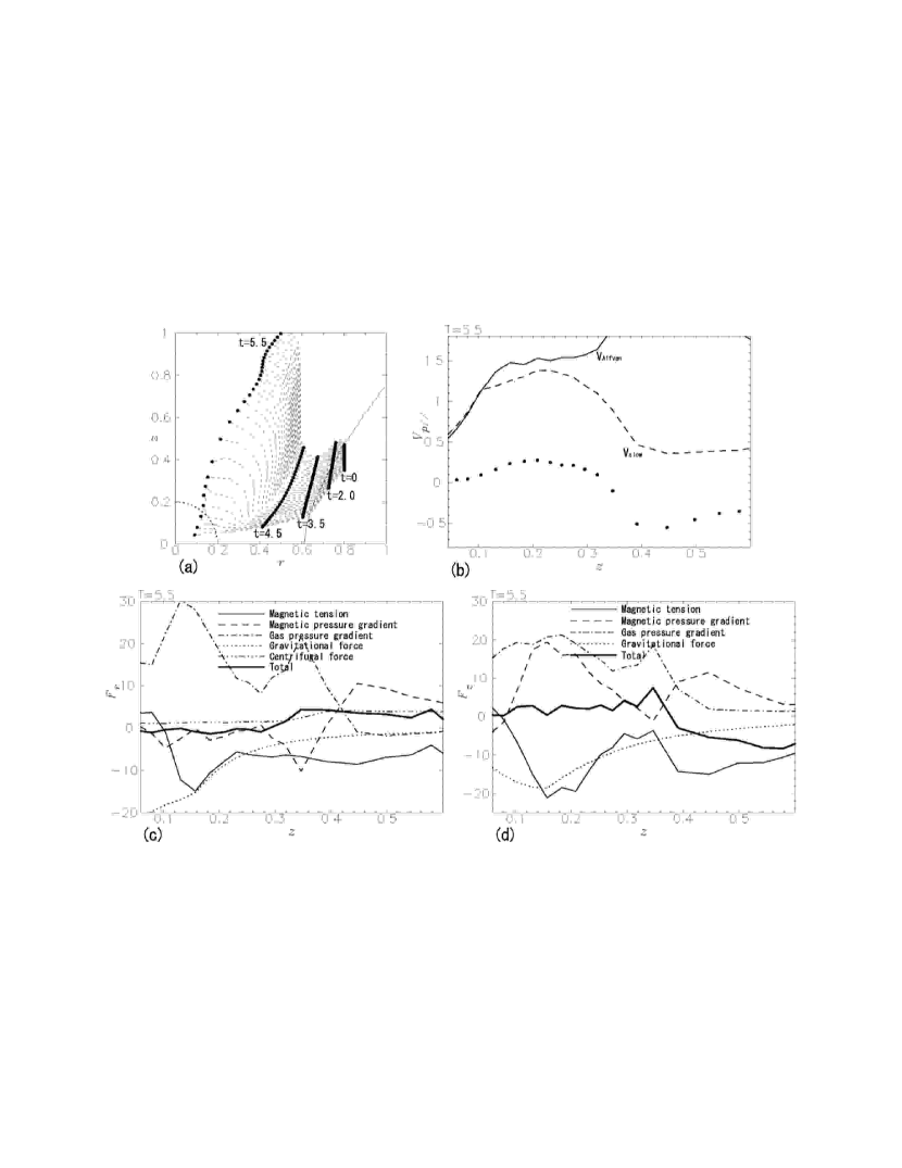
Figure 12: Similar to Fig. 8, but for the model R6. Initial azimuthal position of the Lagrangian fluid elements is 0.

References

- Abramowicz et al. (1978) Abramowicz, M., Jaroszynski, M., & Sikora, M. 1978, A&A, 63, 221
- Asada et al. (2002) Asada, K., Inoue, M., Uchida, Y., Kameno, S., Fujisawa, K., Iguchi, S., & Mutoh, M. 2002, PASJ, 54, L39
- Attridge et al. (1999) Attridge, J. M., Roberts, D. H., & Wardle, J. F. C. 1999, ApJ, 518, L87
- Bacciotti et al. (2002) Bacciotti, F., Ray, T. P., Mundt, R., Eislöffel, J., & Solf, J. 2002, ApJ, 576, 222
- Balbus & Hawley (1991) Balbus, S. A. & Hawley, J. F. 1991, ApJ376, 214
- Balbus & Hawley (1992) Balbus, S. A. & Hawley, J. F. 1992, ApJ400, 610
- Bisnovatyi-Kogan & Lovelace (2001) Bisnovatyi-Kogan, G. S., & Lovelace, R. V. E. 2001, New A Rev., 45, 663
- Blandford (1976) Blandford, R. D. 1976, MNRAS, 176, 465
- Blandford & Payne (1982) Blandford, R. D., & Payne, D. G. 1982, MNRAS, 199, 883
- Bogovalov & Tsinganos (2005) Bogovalov, S., & Tsinganos, K. 2005, MNRAS, 357, 918
- Bridle & Perley (1984) Bridle, A. H., & Perley, R. A. 1984, ARA&A, 22, 319
- Casse & Keppens (2002) Casse, F., & Keppens, R. 2002, ApJ, 581, 988
- Casse & Keppens (2004) Casse, F., & Keppens, R. 2004, ApJ, 601, 90
- Cerqueira & de Gouveia Dal Pino (2001) Cerqueira, A. H., & de Gouveia Dal Pino, E. M. 2001, ApJ, 560, 779
- Coffey et al. (2004) Coffey, D., Bacciotti, F., Woitas, J., Ray, T. P., & Eislöffel, J. 2004, ApJ, 604, 758
- Conway & Murphy (1993) Conway, J. E., & Murphy, D. W. 1993, ApJ, 411, 89
- Curry & Pudritz (1996) Curry, C., & Pudritz, R. E. 1996, MNRAS, 281, 119
- Evans & Hawley (1988) Evans, C. R., & Hawley, J. F. 1988, ApJ, 332, 659
- Fendt & Cemeljic (2002) Fendt, C., & Čemeljić, M. 2002, A&A, 395, 1045
- Ferrari (1998) Ferrari, A. 1998, ARA&A, 36, 539
- Feretti et al. (1999) Feretti, L., Perley, R., Giovannini, G., & Andernach, H. 1999, A&A, 341, 29
- Frank et al. (2000) Frank, A., Lery, T., Gardiner, T. A., Jones, T. W., & Ryu, D. 2000, ApJ, 540, 342
- Fukui et al. (1993) Fukui, Y., Iwata, T., Mizuno, A., Bally, J., & Lane, A. P. 1993, Protostars and Planets III, ed. E. H. Levy & J. Lunine (Tuscon: Univ. Arizona Press), 603
- Furuya et al. (1999) Furuya, R. S., Kitamura, Y., Saito, M., Kawabe, R., & Wootten, H. A. 1999, ApJ, 525, 821
- Gabuzda (2003) Gabuzda, D. C. 2003, New Astronomy Reviews, 47, 599
- Gabuzda et al. (2004) Gabuzda, D. C., Murray, E., & Cronin, P. 2004, MNRAS, 351, L89
- Goldreich et al. (1986) Goldreich, P., Goodman, J., & Narayan, R. 1986, MNRAS, 221, 339
- Hardee & Rosen (1999) Hardee, P. E., & Rosen, A. 1999, ApJ, 524, 650
- Hardee & Rosen (2002) Hardee, P. E., & Rosen, A. 2002, ApJ, 576, 204
- Hawley (1990) Hawley, J. F. 1990, ApJ, 356, 580
- Hawley (2000) Hawley, J. F. 2000, ApJ, 528, 462
- Hawley & Krolik (2001) Hawley, J. F., & Krolik, J. H. 2001, ApJ, 548, 348
- Hawley & Stone (1995) Hawley, J. F., & Stone, J. M. 1995, Comp. Phys. Comm., 89, 127
- Hummel et al. (1992) Hummel, C. A., et al. 1992, A&A, 257, 489
- Hutchison et al. (2001) Hutchison, J. M., Cawthorne, T. V., & Gabuzda, D. C. 2001, MNRAS, 321, 525
- Ibrahim et al. (2004) Ibrahim, A., Sato, K., & Shibata, K. 2004, Progress of Theoretical Physics Supplement, 155, 343
- Kato (2002) Kato, S. X. 2002, Ph.D.thesis, Univ. Tokyo
- Kato et al. (2002) Kato, S. X., Kudoh, T., & Shibata, K. 2002, ApJ, 565, 1035
- Kigure et al. (2002) Kigure, H., Uchida, Y., Nakamura, M., & Hirose, S. 2002, in Proc. of the IAU 8th Asian-Pacific Regional Meeting, Vol. II, ed. S. Ikeuchi, J. Hearnshaw, & T. Hanawa (Tokyo: ASJ), 385
- Kigure et al. (2004) Kigure, H., Uchida, Y., Nakamura, M., Hirose, S., & Cameron, R. 2004, ApJ, 608, 119
- Koide et al. (1999) Koide, S., Shibata, K., & Kudoh, T. 1999, ApJ, 522, 727
- Kotani et al. (1996) Kotani, T., Kawai, N., Matsuoka, M., & Brinkmann, W. 1996, PASJ, 48, 619
- Krasnopolsky et al. (2003) Krasnopolsky, R., Li, Z.-Y., & Blandford, R. D. 2003, ApJ, 595, 631
- Krichbaum et al. (1990) Krichbaum, T. P., Hummel, C. A., Quirrenbach, A., Schalinski, C. J., Witzel, A., Johnston, K. J., Muxlow, T. W. B., & Qian, S. J. 1990, A&A, 230, 271
- Kubo et al. (1998) Kubo, H., Takahashi, T., Madejski, G., Tashiro, M., Makino, F., Inoue, S., & Takahara, F. 1998, ApJ, 504, 693
- Kudoh et al. (1998) Kudoh, T., Matsumoto, R., & Shibata, K. 1998, ApJ, 508, 186
- Kudoh et al. (1999) Kudoh, T., Matsumoto, R., & Shibata, K. 1999, Comput. Fluid Dyn. J., 8, 56
- Kudoh et al. (2002a) Kudoh, T., Matsumoto, R., & Shibata, K. 2002a, PASJ, 54, 121
- Kudoh et al. (2002b) Kudoh, T., Matsumoto, R., & Shibata, K. 2002b, PASJ, 54, 267
- Kudoh & Shibata (1995) Kudoh, T., & Shibata, K. 1995, ApJ, 452, L41
- Kudoh & Shibata (1997a) Kudoh, T., & Shibata, K. 1997a, ApJ, 474, 362
- Kudoh & Shibata (1997b) Kudoh, T., & Shibata, K. 1997b, ApJ, 476, 632
- Kuwabara et al. (2000) Kuwabara, T., Shibata, K., Kudoh, T., & Matsumoto, R. 2000, PASJ, 52, 1109
- Lovelace (1976) Lovelace, R. V. E. 1976, Nature, 262, 649
- Machida & Matsumoto (2003) Machida, M., & Matsumoto, R. 2003, ApJ, 585, 429
- Margon (1984) Margon, B. 1984, ARA&A, 22, 507
- Matsumoto (1999) Matsumoto, R. 1999, in Numerical Astrophysics, ed. S. M. Miyama, K. Tomisaka, & T. Hanawa (Dordrecht: Kluwer), 195
- Matsumoto & Shibata (1997) Matsumoto, R., & Shibata, K. 1997, in ASP Conf. Ser. 121, Accretion Phenomena and Related Outflows, ed. D. T. Wickramasinghe, G. V. Bicknell, & L. Ferrario (San Francisco: ASP), 443
- Matsumoto & Shibata (1999) Matsumoto, R., & Shibata, K. 1999, Adv. Space Res., 23, 1109
- Matsumoto et al. (1996) Matsumoto, R., Uchida, Y., Hirose, S., Shibata, K., Hayashi, M., Ferrari, A., Bodo, G., & Norman, C. 1996, ApJ, 461, 115
- Meier et al. (2001) Meier, D. L., Koide, S., & Uchida, Y. 2001, Science, 291, 84
- Michel (1969) Michel, F. C. 1969, ApJ, 158, 727
- Mirabel & Rodriguez (1994) Mirabel, I. F., & Rodriguez, L. F. 1994 Nature, 371, 46
- Nakamura & Meier (2004) Nakamura, M., & Meier, D. L. 2004, ApJ, 617, 123
- Nakamura et al. (2001) Nakamura, M., Uchida, Y., & Hirose, S. 2001, New Astronomy, 6, 61
- Ogura (1995) Ogura, K. 1995, ApJ, 450, L23
- Ouyed et al. (2003) Ouyed, R., Clarke, D. A., & Pudritz, R. E. 2003, ApJ, 582, 292
- Ouyed & Pudritz (1997a) Ouyed, R., & Pudritz, R. E. 1997, ApJ, 482, 712
- Ouyed & Pudritz (1997b) Ouyed, R., & Pudritz, R. E. 1997, ApJ, 484, 794
- Ouyed & Pudritz (1999) Ouyed, R., & Pudritz, R. E. 1999, MNRAS, 309, 233
- Papaloizou & Pringle (1984) Papaloizou, J. C. B., & Pringle, J. E. 1984, MNRAS, 208, 721
- Proga (2003) Proga, D. 2003, ApJ, 585, 406
- Romanova et al. (1998) Romanova, M. M., Ustyugova, G. V., Koldoba, A. V., Chechetkin, V. M., & Lovelace, R. V. E. 1998, ApJ, 500, 703
- Roos et al. (1993) Roos, N., Kaastra, J. S., & Hummel, C. A. 1993, ApJ, 409, 130
- Sauty et al. (2004) Sauty, C., Trussoni, E., & Tsinganos, K. 2004, A&A, 421, 797
- Shibata (1983) Shibata, K. 1983, PASJ, 35, 263
- Shibata & Kudoh (1999) Shibata, K., & Kudoh, T. 1999, in Proc. of Star Formation 1999, ed. T. Nakamoto (Nagoya: Nobeyama Radio Observatory), 263
- Shibata & Uchida (1986) Shibata, K., & Uchida, Y. 1986, PASJ, 38, 631
- Shibata & Uchida (1987) Shibata, K., & Uchida, Y. 1987, PASJ, 39, 559
- Stirling et al. (2003) Stirling, A. M., et al. 2003, MNRAS, 341, 405
- Stone & Norman (1992) Stone, J. M., & Norman, M. L. 1992, ApJS, 80, 791
- Uchida et al. (2004) Uchida, Y., Kigure, H., Hirose, S., Nakamura, M., & Cameron, R. 2004, ApJ, 600, 88
- Uchida & Shibata (1985) Uchida, Y., & Shibata, K. 1985, PASJ, 37, 515
- Ustyugova et al. (1995) Ustyugova, G. V., Koldoba, A. V., Romanova, M. M., Chechetkin, V. M., & Lovelace, R. V. E. 1995, ApJ, 439, L39
- Ustyugova et al. (1999) Ustyugova, G. V., Koldoba, A. V., Romanova, M. M., Chechetkin, V. M., & Lovelace, R. V. E. 1999, ApJ, 516, 221
- von Rekowski et al. (2003) von Rekowski, B., Brandenburg, A., Dobler, W., & Shukurov, A. 2003, A&A, 398, 825
- Yabe & Aoki (1991) Yabe, T., & Aoki, T. 1991, Comp. Phys. Comm., 66, 219
- Yabe et al. (1991) Yabe, T., Ishikawa, T., Wang, P. Y., Aoki, T., Kadota, Y., & Ikeda, F. 1991, Comp. Phys. Comm., 66, 233
- Zavala & Taylor (2005) Zavala, R. T., & Taylor, G. B. 2005, ApJ, 626, L73