A blind estimation of the angular power spectrum of CMB anisotropy from WMAP

Abstract

Accurate measurements of angular power spectrum of Cosmic Microwave Background (CMB) radiation has lead to marked improvement in the estimates of different cosmological parameters. This has required removal of foreground contamination as well as detector noise bias with reliability and precision. We present the estimation of CMB angular power spectrum from the multi-frequency observations of WMAP using a novel model-independent method. The primary product of WMAP are the observations of CMB in 10 independent difference assemblies (DA) that have uncorrelated noise. Our method utilizes maximum information available within WMAP data by linearly combining all the DA maps to remove foregrounds and estimating the power spectrum from cross power spectra of clean maps with independent noise. We compute $24$ cross power spectra which are the basis of the final power spectrum. The binned average power matches with WMAP team’s published power spectrum closely. A small systematic difference at large multipoles is accounted for by the correction for the expected residual power from unresolved point sources. The correction is small and significantly tempered. Previous estimates have depended on foreground templates built using extraneous observational input. This is the first demonstration that the CMB angular spectrum can be reliably estimated with precision from a self contained analysis of the WMAP data.

1 Introduction

Remarkable progress in cosmology has been made due to the measurements of the anisotropy in the cosmic microwave background (CMB) over the past decade. The extraction of the angular power spectrum of the CMB anisotropy is complicated by foreground emission within our galaxy and extragalactic radio sources, as well, as the detector noise Bouchet & Gispert (1999); Tegmark & Efstathiou (1996). It is established that the CMB follows a blackbody distribution to high accuracy, Mather et al.1994 & (1999). Hence, foreground emissions may be removed by exploiting the fact that their contributions in different spectral bands are considerably different while the CMB power spectrum is same in all the bands Dodelson (1997); Tegmarket al. 2000a ; Bennett et al. 2003b ; Tegmark (1998). Different approaches to foreground removal have been proposed in the literature Bouchet & Gispert (1999); Tegmark & Efstathiou (1996); Hobson et al. (1998)
 Maino et al. 2002, (2003); Eriksen et al. (2005)

The Wilkinson Microwave Anisotropy Probe (WMAP) observes in $5$ frequency bands at $23~{}\rm GHz$ (K), $33~{}\rm GHz$ (Ka), $41~{}\rm GHz$ (Q), $61~{}\rm GHz$ (V) and $94~{}\rm GHz$ (W). In the first data release, the WMAP team removed the galactic foreground signal using a template fitting method based on a model of synchrotron, free free and dust emission in our galaxy Bennett et al. 2003b . The sky map around the galactic plane and around known extragalactic point sources were masked out and the CMB power spectrum was then obtained from cross power spectra of independent difference assemblies in the $41~{}\rm GHz$, $61~{}\rm GHz$ and $94~{}\rm GHz$ foreground cleaned maps Hinshaw et al. 2003a .

A model independent removal of foregrounds has been proposed in the literature
 Tegmark & Efstathiou (1996). The method has also been implemented on the WMAP data in order to create a foreground cleaned map Tegmark et al. (2003). The main advantage of this method is that it does not make any additional assumptions regarding the nature of the foregrounds. Furthermore, the procedure is computationally fast. The foreground emissions are removed by combining the five different WMAP bands by weights which depend both on the angular scale and on the location in the sky (divided into regions based on ‘cleanliness’). However, this analysis did not attempt to remove the detector noise bias Tegmark et al. (2003). Consequently, the power spectrum recovered from the foreground cleaned map has a lot of excess power at large multipole moments due to amplification of detector noise bias beyond the beam resolution.

The prime objective of our paper is to remove detector noise bias exploiting the fact that it is uncorrelated among the different Difference Assemblies (DA) Hinshaw et al. 2003a ; Jarosik et al. (2003). The WMAP data uses 10 DA’s Bennett et al. 2003a ; Bennett et al. 2003c ; Limon et al. ; Hinshaw et al.2003b , one each for K and Ka bands, two for Q band, two for V band and four for W band. We label these as K, Ka, Q1, Q2,V1, V2, W1, W2, W3, and W4 respectively. We eliminate the detector noise bias using cross power spectra and provide a model independent extraction of CMB power spectrum from WMAP first year data. So far, only the $3$ highest frequency channels observed by WMAP have been used to extract CMB power spectrum and the foreground removal has used foreground templates based on extrapolated flux from measurements at frequencies far removed from observational frequencies of WMAP Hinshaw et al. 2003a ; Fosalba & Szapudi (2004); Patanchon et al. (2004). We present a more general procedure where we use observations from all the $5$ frequency channels of WMAP and do not use any extraneous observational input.

2 Methodology

2.1 Foreground Cleaning

Up to the foreground cleaning stage, our method is similar to Tegmark & Efstathiou (1996) and Tegmark et al. (2003). In Tegmark et al. (2003), a foreground cleaned map is obtained by linearly combining 5 maps corresponding to one each for the different WMAP frequency channels. For the Q, V and W frequency channels, where more than one maps were available, an averaged map was used. However, averaging over the DA maps in a given frequency channel precludes any possibility of removing detector noise bias using cross correlation. In our method we linearly combine maps corresponding to a set of 4 DA maps at different frequencies. We treat K and Ka maps effectively as the observation of CMB in two different DA. Therefore we use K and Ka maps in separate combinations. In case of W band 4 DA maps are available. We simply form an averaged map taking two of them at a time and form effectively 6 DA maps. W$ij$ represents simply an averaged map obtained from the $i^{\rm th}$ and $j^{\rm th}$ DA of W band. (Other variations are possible. We defer a discussion to a more detailed publication Saha et al. (2006)). In table 2.1 we list all the $48$ possible linear combinations of the DA maps that lead to ‘cleaned’ maps, C${\bf i}$ and CA${\bf i}$’s, where ${\bf i}$ = 1, 2, …, 24.

(K,KA)+Q1+V1+W12=(C1,CA1)	(K,KA)+Q1+V2+W12=(C13,CA13)
(K,KA)+Q1+V1+W13=(C2,CA2)	(K,KA)+Q1+V2+W13=(C14,CA14)
(K,KA)+Q1+V1+W14=(C3,CA3)	(K,KA)+Q1+V2+W14=(C15,CA15)
(K,KA)+Q1+V1+W23=(C4,CA4)	(K,KA)+Q1+V2+W23=(C16,CA16)
(K,KA)+Q1+V1+W24=(C5,CA5)	(K,KA)+Q1+V2+W24=(C17,CA17)
(K,KA)+Q1+V1+W34=(C6,CA6)	(K,KA)+Q1+V2+W34=(C18,CA18)
(K,KA)+Q2+V2+W12=(C7,CA7)	(K,KA)+Q2+V1+W12=(C19,CA19)
(K,KA)+Q2+V2+W13=(C8,CA8)	(K,KA)+Q2+V1+W13=(C20,CA20)
(K,KA)+Q2+V2+W14=(C9,CA9)	(K,KA)+Q2+V1+W14=(C21,CA21)
(K,KA)+Q2+V2+W23=(C10,CA10)	(K,KA)+Q2+V1+W23=(C22,CA22)
(K,KA)+Q2+V2+W24=(C11,CA11)	(K,KA)+Q2+V1+W24=(C23,CA23)
(K,KA)+Q2+V2+W34=(C12,CA12)	(K,KA)+Q2+V1+W34=(C24,CA24)

Table 1: Different combinations of the DA maps used to obtain the final 48 cleaned maps.

Following the approach of Tegmark & Efstathiou (1996), we introduce a set of weights, ${{\bf[W_{l}]}=(w_{l}^{1},w_{l}^{2},w_{l}^{3},w_{l}^{4})}$ for each of the $4$ DA in the combination, which defines our cleaned map as the linear combination

$$a_{lm}^{\rm Clean}=\sum_{i=1}^{i=4}w_{l}^{i}\frac{a_{lm}^{i}}{B_{l}^{i}}\,,$$ (1)

where $a_{lm}^{i}$ is spherical harmonic transform of map and $B^{i}_{l}$ is the beam function for the channel $i$ supplied by the WMAP team.

The condition that the CMB signal remains untouched during cleaning is encoded as the constraint $\bf[W_{l}][e]=[e]^{T}[W]^{T}=1$ where ${\bf[e]}$ is a $4\times 1$ column vector with unit elements.

Following Tegmark & Efstathiou (1996), Tegmark et al. (2003) and Tegmark et al. (2000a) we obtain the optimum weights which combine $4$ different frequency channels subject to the constraint that CMB is untouched, $\bf[W_{l}]={[e]^{T}[C_{l}]^{-1}}/\left({[e]^{T}[C_{l}]^{-1}[e]}\right)$. Here the matrix ${\bf[C_{l}]}$ is

$${\bf[C_{l}]}\equiv C^{ij}_{l}=\frac{1}{2l+1}\sum_{m=-l}^{m=l}\frac{a^{i}_{lm}a^{j*}_{lm}}{B_{l}^{i}B_{l}^{j}}\,.$$ (2)

In practice, we smooth all the elements of the ${\mathbf{C}_{l}}$ using a moving average window over $\Delta l=11$ before deconvolving by the beam function. This avoids the possibility of an ocassional singular ${\mathbf{C}_{l}}$ matrix. The entire cleaning procedure is automated and takes approximately $3$ hours on a $16$ alpha processor machine to get the $48$ cleaned maps. One of the cleaned maps, C8, is shown in the Fig. 2.1. In all the $48$ maps some residual foreground contamination is visibly present along a small narrow strip on the galactic plane. In a future publication, we assess the quality of foreground cleaning in these maps using the Bipolar power spectrum method Hajian & Souradeep 2003 ; Hajian et al. 2004a ; Hajian & Souradeep (2005) and compare them to others such as the internal Linear combination map (ILC) of WMAP. For the angular power estimation that follows, the Kp2 mask employed suffices to mask the contaminated region in all the $48$ maps.

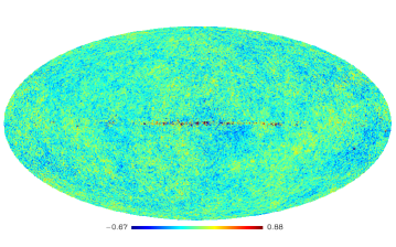
Figure 1: The cleaned map $C8$ for the K, Q2, V2, W13 combination (units ${\rm mK}$). Residual foreground contamination visible along the galactic plane are well within the Kp2 mask that is applied before extracting the angular power spectrum.

2.2 Power Spectrum Estimation

We obtain cross correlated power spectrum from these cleaned maps after applying a Kp2 mask. In choosing pairs Ci & Cj to be cross correlated, we ensure that no DA is common between them. Figure 2.3 lists and plots the $24$ cross power spectra for which the noise bias is zero. The cross power spectra are corrected for effect of the mask, the beam and pixel window. These are accounted for by de-biasing the pseudo-$C_{l}$ estimate using the coupling (bias) matrix corresponding to the Kp2 mask and appropriate circularized beam transform Hivon et al. (2002). Figure 2.3 plots the $24$ cross power spectra (binned) individually. The spectra closely match each other for $l<540$. The $24$ cross power spectra are then combined with equal weights into a single ‘Uniform average’ power spectrum  . We also estimate the residual power contamination in the ‘Uniform average’ power spectrum from the unresolved point sources on running through our analysis the same source model used by WMAP team to correct for this contaminant Hinshaw et al. 2003a . The model is derived entirely within the WMAP data based on fluxes and spectra of $208$ resolved point sources identified in the maps Bennett et al. 2003b . The residual power from unresolved point sources is a constant offset of $\sim 140\mu K^{2}$ for $l\mathrel{\hbox to0.0pt{\lower 4.0pt\hbox{\hskip 1.0pt$\sim$}\hss}\raise 1.0pt\hbox{$>$}}400$ (and negligible at lower $l$). This residual is much less than actual point source contamination in Q, KA or K band and intermediate between V and W band point source contamination. It is noteworthy that the method significantly tempers the point source residual at large $l$ that otherwise is $\propto l^{2}$ in each map. The final power spectrum is binned in the same manner as the WMAP’s published result for ease of comparison.

2.3 Error Estimate on the Power Spectrum

The errors on the final power spectrum are computed from $110$ random Monte Carlo simulations of CMB maps for every DA each with a realization based on corresponding WMAP noise map (available at LAMBDA) and diffuse foreground contamination. The common CMB signal in all the maps was based on a realization of the WMAP ‘power law’ best fit $\Lambda$-CDM model Spergel et al. (2003). We use the publicly available Planck Sky Model to simulate the contamination from the diffuse galactic (synchrotron, thermal dust and free-free) emission at the WMAP frequencies. The CMB maps were smoothed by the beam function appropriate for each WMAP’s detector. The set of DA maps corresponding to each realizations were passed through the same pipeline used for the real data. Averaging over the $110$ power spectra we recover the model power spectrum, but for a hint of bias towards lower values in the low $l$ moments. For $l=2$ and $l=3$ the bias is $-27.4\%$ and $-13.8\%$ respectively. However this bias become negligible at higher $l$, e.g. at $l=22$, it is only $-0.8\%$.

The standard deviation obtained from the diagonal elements of the covariance matrix is used as the error bars on the $C_{l}$’s obtained from the data. (The beam uncertainty is not included here, but is deferred to future work where we also incorporate non-circular beam corrections Mitra et al. (2004).)

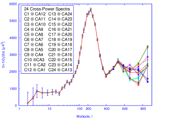
Figure 2: The $24$ individual cross power spectra corresponding to the cross correlations listed in this figure are plotted. The cross spectra show very small dispersion for $l\mathrel{\hbox to0.0pt{\lower 4.0pt\hbox{\hskip 1.0pt$\sim$}\hss}\raise 1.0pt\hbox{$<$}}540$. The average power spectrum is plotted in red line and blue error bars. The multipole range is on log scale for $l<100$, and linear, thereafter.

3 Results

We obtain a ‘Uniform average’ power spectrum of the 24 cross spectrum following the method mentioned in section 2.2. The black curve in Fig. 3 compares our results with the WMAP published power spectrum plotted with red line. The power spectra from two independent analysis are reasonably close. In case of ‘Uniform average’ a maximum difference of $92~{}\mu K^{2}$ is observed only for octopole. For the large multipole range the difference is small and for $l=752$ it is approximately $48~{}\mu K^{2}$. This is well within the $1\sigma$ error bar ($510\mu K^{2}$ ) obtained from the simulation. The small, but systematic excess, at large multipoles is precisely resolved when our ‘Uniform average’ is corrected for the expected residual power from unresolved point source contamination described in $\S$2.2. The point source corrected power spectrum is shown in black line in this figure. The difference of this power spectrum with the published WMAP estimate is shown in the bottom panel of Fig. 3. The differences are well within the $1\sigma$ error-bars estimated from the simulations described in $\S$2.3.

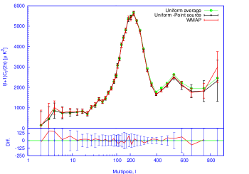
Figure 3: The ‘Uniform average power spectrum is plotted in green line. The black line shows residual unresolved point source corrected power spectrum. The error-bars are computed from the diagonal elements of the covariance matrix obtained from our simulation pipeline. Beyond $l=400$ all the error bars are shifted by $\delta l=10$ to visually distinguish between error bars obtained from our method and the WMAP’s published error bars. The published binned WMAP power spectrum is plotted in red line with error bars. The multipole range $2<l<100$ are plotted in the log scale to show the small $l$ behavior of the power spectrum.

We find a suppression of power in the quadrupole and octopole moments consistent with WMAP published result. However, our quadrupole moment ($146\mu K^{2}$) is a little larger than the WMAP’s quadrupole moment ($123\mu K^{2}$) and Octopole ($455\mu K^{2}$) is less than WMAP’s result ($611\mu K^{2}$). The ‘Uniform average’ power spectrum does not show the ‘bite’ like feature present in WMAP’s power spectrum at the first acoustic peak reported by WMAP Hinshaw et al. 2003a . We perform a quadratic fit to the peaks and troughs of the binned spectrum similar to WMAP analysis Page et al. (2003). For the residual point source corrected (‘Uniform average’) power spectrum we obtain the first acoustic peak at $l=219.8\pm 0.8$ $(220.8\pm 0.8)$ with amplitude $\Delta T_{l}=74.1\pm 0.3\mu K$ $(74.4\pm 0.3\mu K)$, the second acoustic peak at $l=544\pm 17$ $(545\pm 17)$ with amplitude $\Delta T_{l}=48.3\pm 1.2\mu K$ $(49.6\pm 1.2\mu K)$ and the first trough at $l=419.2\pm 5.6$ $(418.7\pm 5.5)$ with amplitude $\Delta T_{l}=41.7\pm 1$ $\mu K(42.2\pm 0.9\mu K)$.

As cross checks of the method, we have carried out analysis with other possible combinations of the DA maps.

1. The WMAP team also provide foreground cleaned maps corresponding to Q1 to W4 DA (LAMBDA). The Galactic foreground signal, consisting of synchrotron, free-free, and dust emission, was removed using the 3-band, 5-parameter template fitting method Bennett et al. 2003b . We also include K and Ka band maps which are not foreground cleaned. The resulting power spectrum from our analysis matches closely to the ‘Uniform average’ power spectrum.

2. Excluding the K and Ka band from our analysis we get a power spectrum close to the ‘Uniform average’ results. Notably, we find a more prominent notch at $l=4$ similar to WMAP’s published results.

This is a clear demonstration that the blind approach to foreground cleaning is comparable in efficiency to that from template fitting methods and certainly adequate for a reliable estimation of the angular power spectrum.

4 Conclusion

The rapid improvement in the sensitivity and resolution of the CMB experiments has posed increasingly stringent requirements on the level of separation and removal of the foreground contaminants. Standard approaches to foreground removal, usually incorporate the extra information about the foregrounds available at other frequencies, the spatial structure and distribution in constructing a foreground template at the frequencies of the CMB measurements. These approach could be susceptible to uncertainties and inadequacies of modeling involved in extrapolating from the frequency of observation to CMB observations.

We carry out an estimation of the CMB power spectrum from the WMAP first year data that is independent of foreground model and evades these uncertainties. The novelty is to make clean maps from the difference assemblies and exploit the lack of noise correlation between the independent channels to eliminate noise bias. This is the first demonstration that the angular power spectrum of CMB anisotropy can be reliably estimated with precision solely from the WMAP data (difference assembly maps) without recourse to any external data.

The understanding of polarized foreground contamination in CMB polarization maps is rather scarce. Hence modeling uncertainties could dominate the systematics error budget of conventional foreground cleaning. The blind approach extended to estimating polarization spectra after cleaning CMB polarization maps could prove to be particularly advantageous.

5 Acknowledgment

The analysis pipeline as well as the entire simulation pipeline is based on primitives from the Healpix package. We acknowledge the use of version 1.1 of the Planck reference sky model, prepared by the members of Working Group 2 and available at www.planck.fr/heading79.html. The entire analysis procedure was carried out on the IUCAA HPC facility. RS thanks IUCAA for hosting his visits. We thank the WMAP team for producing excellent quality CMB maps and making them publicly available. We thank Amir Hajian, Subharthi Ray and Sanjit Mitra in IUCAA for helpful discussions. We are grateful to Lyman Page, Olivier Dore, Francois Bouchet, Simon Prunet, Charles Lawrence and an anonymous referee for thoughtful comments and suggestions on this work. PJ and RS thank Sudeep Das for collaborating during the initial stages of this project.

References

- (1) Bennett, C. L.et al. 2003a, ApJS, 148, 1
- (2) Bennett, C. L.et al. 2003b, ApJS, 148, 97
- (3) Bennett, C. L.et al. 2003c, ApJ, 583, 1
- Bouchet & Gispert (1999) F. R. Bouchet and R. Gispert, New Astronomy 4,443, (1999).
- Calabretta et al. (2004) Calabretta, M. R., astro-ph/0412607
- Dodelson (1997) Dodelson, S.1997, ApJ, 482, 577
- Eriksen et al. (2005) Eriksen, H. K. et al. 2005, preprint (astro-ph/0508268).
- Fosalba & Szapudi (2004) Fosalba, P., & Szapudi, I.2004, ApJ, 617,, 95
- (9) Gorski, K. M. et al. 1999a astro-ph/9905275
- (10) Gorski, K. M. et al. 1999b astro-ph/9812350.
- (11) Hajian, A. et al.2004a, ApJ, 618, 63
- Hajian & Souradeep (2005) Hajian, A., Souradeep, T., astro-ph/0501001
- (13) Hajian, A.,Souradeep, T.2003 ApJ, 597, 5
- (14) Hinshaw, G.et al.2003, ApJS, 148, 135
- (15) Hinshaw, G.et al.2003a,ApJS, 148, 63
- Hivon et al. (2002) Hivon, E.et al. 2002, ApJ, 567, 2-17
- Hobson et al. (1998) Hobson, M. P. et al. 1998, MNRAS, 300, 1
- Jarosik et al. (2003) Jarosik, N. 2003, et al., ApJS, 145, 413
- (19) M. Limon, et al., Wilkinson Microwave Anisotropy Probe (WMAP): Explanatory Supplement, version 1.0, at the LAMBDA website.
- Mather et al.1994 & (1999) Mather, J. et al.1994, ApJ, 420, 439; ibid. 1999, ApJ, 512, 511
- Maino et al. 2002, (2003) Maino, D. et al. 2002, MNRAS, 334, 53; ibid, MNRAS, 344, 544
- Mitra et al. (2004) Mitra, S. et al.2004, Phys. Rev. D, 70, 103002
- Page et al. (2003) Page, L. et al, 2003, ApJS, 148, 233
- Patanchon et al. (2004) Patanchon, G., Cardoso, J. F., Delabrouille, J., & Vielva, P.2004, astro-ph/0410280