The impact of halo shapes on the bispectrum in cosmology

Abstract

We use the triaxial halo model formalism of Smith & Watts (2005) to investigate the impact of dark matter halo shapes on the cosmological bispectrum. Analytic expressions for the dark matter distribution are derived and subsequently evaluated through numerical integration. Two models for the ellipsoidal halo profiles are considered: a toy model designed to isolate the effects of halo shape on the clustering alone; and the more realistic model of Jing & Suto (2002). For equilateral $k$-space triangles, we show that the predictions of the triaxial model are suppressed, relative to the spherical model, by up to $\sim 7\%$ and $\sim 4\%$ for the two profiles respectively. When one considers the reduced bispectrum as a function of triangle configuration it is found to be highly sensitive to halo shapes on small scales. The generic features of our predictions are that, relative to the spherical halo model, the signal is suppressed for $k$-vector configurations that are close to equilateral triangles and boosted for configurations that are colinear. This appears to be a unique signature of halo triaxiality and potentially provides a means for measuring halo shapes in forthcoming cosmic shear surveys.

The galaxy bispectrum is also explored. Two models for the halo occupation distribution (HOD) are considered: the binomial distribution of Scoccimarro et al. (2001) and the Poisson satellite model of Kravtsov et al. (2004). Our predictions show that the galaxy bispectrum is also sensitive to halo shapes, although relative to the mass the effects are reduced. The HOD of Kravtsov et al. is found to be more sensitive. This owes to the fact that the first moment of the occupation probability is a steeper function of mass in this model, and hence the high mass (more triaxial) haloes are more strongly weighted. Interestingly, the functional form of the configuration dependent bispectrum is, modulo an amplitude shift, not strongly sensitive to the exact form of the HOD, but is mainly determined by the halo shape. However, a combination of measurements made on different scales and for different $k$-space triangle configurations is sensitive to both halo shape and the HOD.

1 Introduction

In our current picture of structure formation, small Cold Dark Matter (CDM) density fluctuations, seeded during an early epoch of cosmic inflation, collapse through gravitational instability. From an initial spectrum of fluctuations that is almost scale-invariant, the collapse proceeds in a hierarchical way with fluctuations on small scales collapsing at early times to form dense clumps of dark matter (haloes), and with those on larger scales collapsing at later times. This gives rise to a web-like network of filaments and clusters – the ‘cosmic web’ (Bond & Myers, 1996). Current observational constraints strongly suggest that the growth of structure takes place in a Universe that is flat and which at late times is dominated by an unknown Dark Energy component that drives an accelerated Universal expansion (Spergel et al., 2003). Building a complete statistical description of the clustering pattern of the dark matter is consequently of great importance: this may provide detailed information concerning the physics of the dark matter, the statistics of the primordial fluctuations and also valuable insight into the nature of dark energy. Direct comparison of the dark matter distribution with that of the galaxies reveals the salient physics of galaxy formation.

However, the dynamics of structure formation are nonlinear and analytic solutions for the equations of motion are only tractable for highly idealized cases. Robust calculation of the CDM density field therefore requires recourse to numerical integration via $N$-body methods. Over the past decades significant effort has been invested in performing and analyzing large numerical simulations. The results of this have led to a number of semi-empirical formulae that describe the dark matter halo phenomenology to high accuracy. In particular, halo abundances (Sheth & Tormen, 1999; Jenkins et al., 2001), large-scale bias (Mo & White, 1996; Sheth & Tormen, 1999), density structures (Navarro, Frenk & White, 1997 – hereafter NFW; Bullock et al., 2001; Power et al., 2003; Jing & Suto, 2002 – hereafter JS02), internal velocity distributions and large scale velocity bias (Sheth et al., 2001a, b; Sheth & Diaferio, 2001) are now well characterized. More recently, attention has been focused on quantifying halo shapes (JS02), substructure phenomenology (Moore et al., 1999; Klypin et al., 1999; Ghigna et al., 2000) and effects on the halo due to baryon physics (Gnedin et al., 2004; Kazantzidis et al., 2004). Collectively, these ideas have lead to the development and evolution of the halo model paradigm for structure formation.

In the most basic formulation of the halo model (Seljak, 2000; Peacock & Smith, 2000; Ma & Fry, 2000), one assumes that all of the dark matter in the Universe is confined to virialized, spherical haloes that possess some distribution in mass, some universal density structure and a large-scale bias derivable from perturbation theory, all of which are characterizable through the halo mass. The clustering statistics over all scales then conveniently break down into terms involving correlations between haloes and correlations within haloes. This approach has had a high degree of success in modelling the low-order spatial clustering statistics of the mass. Most advantageously, the halo model can also be used to make predictions for the clustering statistics of the galaxy distribution, which in general can be thought of as a biased sampling of the underlying mass distribution. Indeed, in the halo picture the concept of bias is replaced with that of the Halo Occupation Distribution (HOD), which dictates the number and position of galaxies within dark matter haloes (Berlind & Weinberg, 2002). Moreover, the HOD connects in a satisfying manner to both the theoretical predictions of galaxy formation models (Benson et al., 2000; Seljak, 2000; Scoccimarro et al., 2001 – hereafter SSHJ; Berlind & Weinberg, 2002, and others) and direct observational reality (Peacock & Smith, 2000; Berlind & Weinberg, 2002; Yang, Mo & van den Bosch, 2003, and others).

Whilst the agreement between the halo model and numerical simulations is in general good at the two-point level, significant differences have been reported at the three-point level (SSHJ; Fosalba, Pan & Szapudi, 2005). Although a recent study by Wang et al. (2004) showed that the spherical halo model could be modified to provide a better fit to simulation data, if a finite volume correction and a somewhat arbitrary spatial exclusion scale for the haloes were taken into account. However, discrepancies still remain discernible on both small and large scales. It is currently believed that the various inconsistencies between the halo model and N-body simulations are manifestations of the breakdown of key assumptions in the model. Thus, given the significant interest in this halo based approach, it is of crucial importance to understand the validity of all its approximations. In particular, these issues must be addressed if we are to take seriously the halo model as a tool for precision cosmology.

One possible erroneous assumption is that dark matter haloes are spherical, or rather, that we may work with the spherical averages of the density profiles. However, it has long been known that the haloes found in numerical simulations are more closely described as triaxial ellipsoids (Barnes & Efstathiou, 1987; Frenk et al., 1988; Warren et al., 1992). Recently, JS02 have shown, through high resolution $N$-body simulations, that the inclusion of halo shape information into the modelling of the density structure leads to improved fitting functions. With these ideas in mind, some key questions can now be asked: To what extent do the shapes of the dark matter haloes affect the clustering statistics of the mass distribution? Is there any observable affect on the galaxy clustering?

In a recent paper, Smith & Watts (2005, hereafter SW05) laid out the foundations for performing halo model calculations with triaxial haloes: the ‘triaxial halo model’. They then went on to calculate the importance of halo shapes on the dark matter power spectrum, the Fourier transform of the two-point correlation function. They reported that the effect of halo triaxiality was to suppress the power spectrum on small/nonlinear scales at the level of between $\sim$ 5% and $\sim$ 15%, dependent on the precise choice of density profile model.

A number of other modifications to the halo model may lead to similar effects on the power spectrum. Particular examples are the inclusion of a stochastic concentration parameter in halo density profiles (Cooray & Hu, 2001) and the treatment of halo substructure (Sheth & Jain, 2003; Dolney, Jain & Takada, 2004). More recently, some have suggested that changes to the halo boundary definition may affect significant changes to the clustering (Takada & Jain, 2003a; Fosalba, Pan & Szapudi, 2005). Clearly, if one wishes to disentangle these effects one must look to higher order statistics. In this paper we apply the triaxial halo model formalism of SW05 to the task of computing the bispectrum, the Fourier space analog of the three-point correlation function. The bispectrum is considered to be the lowest order spatial statistic that is sensitive to the shapes of structures. We will demonstrate that this measure can indeed be used to differentiate between changes to halo density profiles and changes to halo shapes.

The paper breaks down as follows: In Section 2 we review some theoretical notions and lay down the bones of the triaxial halo model formalism. In Section 3 we provide the details of our derivation of the three-point correlation and bispectrum for the mass, presenting the results in Section 4. In Section 5 we switch from mass clustering to galaxy clustering and repeat the analysis for galaxies. Finally, we discuss our findings and draw our conclusions in Section 6.

Throughout we assume a flat, dark energy dominated cosmological model with equation of state manifest as a cosmological constant. We take $\Omega_{m}=0.3$ and $\Omega_{DE}=0.7$, where $\Omega_{m}$ and $\Omega_{DE}$ are the ratios of the density in dark matter and dark energy to the critical density, respectively. We use the linear power spectrum of Efstathiou, Bond & White (1992) with normalization $\sigma_{8}=0.9$ and shape parameter $\Gamma\equiv\Omega_{m}h=0.21$, where $h=0.7$ is the dimensionless Hubble parameter.

2 Theoretical background

2.1 three-point spatial clustering statistics

In this paper we are concerned with the three-point spatial statistics of the density contrast field $\delta({\bf r})$. This field is defined through the relation

$$\rho({\bf r})=\bar{\rho}\left[1+\delta({\bf r})\right],$$ (1)

where $\rho({\bf r})$ is the physical density and $\bar{\rho}$ is the density of the background. The three-point correlation function, $\zeta$, is defined as the ensemble average of $\delta$ measured at three points in space. This can be written

$$\zeta({\bf r}_{1},{\bf r}_{2},{\bf r}_{3})\equiv\left<\delta({\bf r}_{1})\,\delta({\bf r}_{2})\,\delta({\bf r}_{3})\right>,\$$ (2)

where the angled brackets denote the ensemble average. For homogeneous random fields $\zeta$ obeys translational invariance:

$$\zeta({\bf r}_{1},{\bf r}_{2},{\bf r}_{3})=\zeta({\bf r}_{1}+{\bf r}_{0},{\bf r}_{2}+{\bf r}_{0},{\bf r}_{3}+{\bf r}_{0}),$$ (3)

where ${\bf r}_{0}$ is an arbitrary position vector. For isotropic random fields, $\zeta$ also obeys rotational invariance:

$$\zeta({\bf r}_{1},{\bf r}_{2},{\bf r}_{3})=\zeta({\mathcal{R}}{\bf r}_{1},{\mathcal{R}}{\bf r}_{2},{\mathcal{R}}{\bf r}_{3}),$$ (4)

where ${\mathcal{R}}$ represents an arbitrary coordinate rotation. For universes that obey the cosmological principle these two properties must hold. Lastly, $\zeta$ must also be invariant under parity transformations:

$$\zeta({\bf r}_{1},{\bf r}_{2},{\bf r}_{3})=\zeta(-{\bf r}_{1},-{\bf r}_{2},-{\bf r}_{3})\ .$$ (5)

In what follows, we will not deal explicitly with $\zeta$, but instead work with its Fourier transformed counterpart, the bispectrum $B$,

$$\left<\delta({\bf k}_{1})\delta({\bf k}_{2})\delta({\bf k}_{3})\right>=(2\pi)^{3}B({\bf k}_{1},{\bf k}_{2},{\bf k}_{3})\,{\delta^{D}}({\bf k}_{1}+{\bf k}_{2}+{\bf k}_{3})\ ,$$ (6)

where $\delta({\bf k})$ is the Fourier transform of $\delta({\bf r})$ and ${\delta^{D}}$ is the Dirac delta function. From the argument of the delta function we obtain the triangle condition, i.e that the sum of the three wave-vectors ${\bf k}_{1}$, ${\bf k}_{2}$ and ${\bf k}_{3}$ form the null vector. The bispectrum and three-point correlation function are explicitly related through

$$\zeta({\bf r}_{1},{\bf r}_{2},{\bf r}_{3})=\int\frac{d{\bf k}_{1}}{(2\pi)^{3}}\frac{d{\bf k}_{2}}{(2\pi)^{3}}\,\,B({\bf k}_{1},{\bf k}_{2},-{\bf k}_{1}-{\bf k}_{2})$$

$$\hskip 45.52458pt\times\exp{[-\rm i{\bf k}_{1}\cdot({\bf r}_{1}-{\bf r}_{3})]}\exp{[-\rm i{\bf k}_{2}\cdot({\bf r}_{2}-{\bf r}_{3})]}.$$ (7)

From the reality of $\zeta$, we find that

$$B({\bf k}_{1},{\bf k}_{2},{\bf k}_{3})=B^{*}(-{\bf k}_{1},-{\bf k}_{2},-{\bf k}_{3})\ ,\$$ (8)

where ^∗ denotes complex conjugation and henceforth the triangle condition is to be assumed. If the $\delta$-field is statistically homogeneous and isotropic, then following equation (5) the bispectrum also obeys parity invariance:

$$B({\bf k}_{1},{\bf k}_{2},{\bf k}_{3})=B(-{\bf k}_{1},-{\bf k}_{2},-{\bf k}_{3})\ .$$ (9)

This, combined with the reality constraint of equation (8) implies that the bispectrum is real. Lastly, following equation (4) the bispectrum is also rotationally invariant:

$$B({\bf k}_{1},{\bf k}_{2},{\bf k}_{3})=B({\mathcal{R}}{\bf k}_{1},{\mathcal{R}}{\bf k}_{2},{\mathcal{R}}{\bf k}_{3})\ .$$ (10)

2.2 Ellipsoidal systems

In what follows we will be concerned with the clustering properties of triaxial dark matter haloes. We therefore define some important relations for these objects (see Chandrasekhar, 1969, for a full treatise). Consider a heterogeneous triaxial ellipsoid that has semi-axis lengths $a$, $b$ and $c$, where $a\leq b\leq c$, and orthogonal principle axis vectors $(\hat{\bf{e}}_{a},\hat{\bf{e}}_{b},\hat{\bf{e}}_{c})$. We define the triaxial coordinate system $(R,\Theta,\Phi)$ with respect to the principle axes of the halo, where $\hat{\bf{e}}_{c}$ is taken to be in the $z$-direction of a standard Cartesian system. The radial parameter $R$ traces out thin iso-density shells, or homoeoids, and the parameters $\Theta$ and $\Phi$ are the polar and azimuthal angles respectively. In this system the Cartesian components can be written

$$x=\frac{a}{c}R\cos\Phi\sin\Theta\ ;\ y=\frac{b}{c}R\sin\Phi\sin\Theta\ ;\ z=R\cos\Theta.$$ (11)

It is to be noted that the ellipsoidal angles differ from those of the spherical coordinate system. The parameter $R$ can be related to the Cartesian coordinates and axis ratios through

$$\frac{R^{2}}{c^{2}}=\frac{x^{2}}{a^{2}}+\frac{y^{2}}{b^{2}}+\frac{z^{2}}{c^{2}}\ .$$ (12)

The benefits of this choice of coordinate system are now apparent: if all homoeoidal shells are concentric, and if one picks coordinates with the same axis ratios as the triaxial ellipsoid, then the density run of the ellipsoid can be described by a single parameter:

$$\rho({\bf r})\rightarrow\rho(R)\ .$$ (13)

Furthermore, the mass enclosed within some iso-density cut-off scale $R_{\rm cut}$, can be obtained most simply by

$$M=\int_{R_{\rm cut}({\bf r})}d{\bf r}\rho({\bf r})=4\pi\frac{ab}{c^{2}}\int_{0}^{R_{\rm cut}}dRR^{2}\rho(R)\ ,$$ (14)

where the ellipsoidal coordinates have allowed us to circumvent the problem of evaluating complicated halo boundaries.

It is now also convenient to define what we mean by a halo: any object that has a volume averaged over-density 200 times the background density is considered to be a gravitationally bound halo of dark matter. This leads directly to the following relation between the mass, radius and axis ratios

$$M_{200}=\frac{4}{3}\pi R_{200}^{3}{\left(\frac{ab}{c^{2}}\right)}200\bar{\rho}\ .$$ (15)

The above definition was adopted in order to be consistent with the mass-function of Sheth & Tormen (1999).

2.3 Triaxial halo model

We next summarize the theoretical ingredients of the triaxial halo model presented in SW05. Consider a density field comprised entirely of ellipsoidal dark matter haloes of different masses. The density run of each halo is specified by some universal profile, the exact details of which are not important at this stage save that the general properties discussed in the previous section are satisfied. Each halo may therefore be characterized by a set of stochastic variables. These are the position vector for the halo centre of mass, ${\bf x}$, the mass $M$, the principle axis lengths $(a,b,c)$, and the direction vectors for these axes $(\hat{\bf{e}}_{a},\hat{\bf{e}}_{b},\hat{\bf{e}}_{c})$. We express these last two sets of variables compactly by using the notation ${\bf a}\equiv(a,b,c)$ and $\mbox{\boldmath$\mathcal{E}$}\equiv(\hat{\bf{e}}_{a},\hat{\bf{e}}_{b},\hat{\bf{e}}_{c})$. Thus, the density at any point ${\bf r}$ can be expressed as a sum over the $N$ haloes that comprise the field

$$\rho({\bf r})=\sum_{i}^{N}M_{i}\,U({\bf r}-{\bf x}_{i},M_{i},\mbox{\boldmath$\mathcal{E}$}_{i},{\bf a}_{i}),$$ (16)

where $U$ is the mass normalized density profile and where sub-scripts $i$ denote the characteristics of the $i^{\rm th}$ halo.

The correlation functions of the density field follow directly from taking ensemble averages of products of the density at different points in space. To compute the ensemble averages we integrate over the joint probability density function (hereafter PDF) for the $N$ haloes that form the density field, and sum over the probabilities for obtaining the $N$ haloes (see McClelland & Silk, 1977, for a similar approach)

$$\langle\cdot\cdot\cdot\rangle\equiv\sum_{j}p(N_{j}|V)\int\prod_{i=1}^{N_{j}}dM_{i}\;d{\bf x}_{i}\;d{\bf a}_{i}\;d\mbox{\boldmath$\mathcal{E}$}_{i}$$

$$\hskip 8.5359pt\times\ p(M_{1},..,M_{N_{j}},{\bf x}_{1},..,{\bf x}_{N_{j}},{\bf a}_{1},..,{\bf a}_{N_{j}},\mbox{\boldmath$\mathcal{E}$}_{1},..,\mbox{\boldmath$\mathcal{E}$}_{N_{j}}|N_{j})\ .$$ (17)

Provided the volume of space considered is large, then $p(N|V)$ is very sharply spiked around $N=\bar{n}V\gg 1$, where $\bar{n}$ is the mean number density of haloes. We restrict our study to this case only.

The integrals over $\mathcal{E}$ in equation (17) represent averages over all possible orientations of the halo. The orientation of the halo frame can be specified relative to a fixed Cartesian basis set through the Euler angles. These represent successive rotations of the halo frame about the $z$–axis by $\alpha$, the $y^{\prime}$–axis by $\beta$, and the $z^{\prime\prime}$–axis by $\gamma$ (see Mathews & Walker, 1970). Hence, the process of averaging over all halo orientations can be performed by integrating over all Euler angles. We thus make the following transformation $\mbox{\boldmath$\mathcal{E}$}\rightarrow(\alpha,\beta,\gamma)$.

Finally, we will require explicit expressions for the joint PDF for a single halo’s characteristics, $p({\bf x},M,\mbox{\boldmath$\mathcal{E}$},{\bf a})$. If we assume that a halo’s orientation, position and mass are independent random variables, and that the halo axis ratios are dependent on mass only (see e.g JS02), then we may write

$$p({\bf x},M,\mbox{\boldmath$\mathcal{E}$},{\bf a})=\frac{1}{V}\frac{n(M)}{\bar{n}}p(\mbox{\boldmath$\mathcal{E}$})p({\bf a}|M),$$ (18)

where $n(M)$ is the mass function of haloes. If the orientation of a halo is uniformly random on the sphere then $p(\mbox{\boldmath$\mathcal{E}$})=1/8\pi^{2}$ (see SW05 for further details).

3 Clustering of triaxial haloes

3.1 The three-point correlation function

We are now in a position to compute the three-point correlation function $\zeta({\bf r}_{1},{\bf r}_{2},{\bf r}_{3})$ in the triaxial halo model. This is done by applying the machinery of equations (16) and (17), to the definitions given by equation (2) in conjunction with equation (1) – see also SW05. We find that, as for the case of the standard halo model, $\zeta$ can be expressed as the sum of three terms

$$\zeta=\zeta^{1{\rm H}}+\zeta^{2{\rm H}}+\zeta^{3{\rm H}}\ ,$$ (19)

where we have suppressed the position vector dependence for simplicity. Here $\zeta^{1{\rm H}}$, $\zeta^{2{\rm H}}$ and $\zeta^{3{\rm H}}$ give the contributions for the case where: all three points are within the same halo; two points are within the same halo and the third is within a separate halo; all three points are within distinct haloes. Throughout, we refer to these contributions as the 1-, 2- and 3-Halo terms. These have the following forms:

$$\zeta^{1{\rm H}}=\frac{1}{\bar{\rho}^{3}8\pi^{2}}\int dM\;d{\bf x}\;d{\bf a}\;d\mbox{\boldmath$\mathcal{E}$}\;\;M^{3}\;n(M)p({\bf a}|M)$$

$$\hskip 28.45274pt\times\prod_{i=1}^{3}\left\{U(M,{\bf x}-{\bf r}_{i},{\bf a},\mbox{\boldmath$\mathcal{E}$})\right\}\;\ ;$$ (20)

$$\zeta^{2{\rm H}}=\frac{1}{\bar{\rho}^{3}(8\pi^{2})^{2}}\int\prod_{i=1}^{2}\left\{dM_{i}\,d{\bf x}_{i}\,d{\bf a}_{i}\,d\mbox{\boldmath$\mathcal{E}$}_{i}\,n(M_{i})\,p({\bf a}_{i}|M_{i})\right.$$

$$\hskip 28.45274pt\times\left.\ U({\bf x}_{i}-{\bf r}_{i},M_{i},{\bf a}_{i},\mbox{\boldmath$\mathcal{E}$}_{i})\right\}M_{1}^{2}\,M_{2}$$

$$\hskip 28.45274pt\times\ \,U({\bf x}_{1}-{\bf r}_{3},M_{1},{\bf a}_{1},\mbox{\boldmath$\mathcal{E}$}_{1})\;\xi^{s}(1,2)+{\rm cyc}\ ;$$ (21)

$$\zeta^{3{\rm H}}=\frac{1}{\bar{\rho}^{3}(8\pi^{2})^{3}}\int\prod_{i=1}^{3}\left\{dM_{i}\;d{\bf x}_{i}\;d{\bf a}_{i}\;d\mbox{\boldmath$\mathcal{E}$}_{i}\;M_{i}n(M_{i})\,p({\bf a}_{i}|M_{i})\right.$$

$$\hskip 28.45274pt\times\,\left.U({\bf x}_{i}-{\bf r}_{i},M_{i},{\bf a}_{i},\mbox{\boldmath$\mathcal{E}$}_{i})\right\}\,\zeta^{s}(1,2,3)\ .$$ (22)

In deriving this result we have used the fact that the joint PDF for the characteristics of three haloes may be rewritten

$$p(1,2,3)=p(1)\,p(2)\,p(3)\left[1+\xi^{s}(1,2)+\xi^{s}(2,3)\right.$$

$$\hskip 42.67912pt\left.+\xi^{s}(3,1)+\zeta^{s}(1,2,3)\right]\ ,$$ (23)

where we have used the short-hand notation $p(1)\equiv p({\bf x}_{1},M_{1},{\bf a}_{1},\mbox{\boldmath$\mathcal{E}$}_{1})$ etc. The quantity $p(1)$ is the 1-Halo PDF, as given by equation (18), while $\xi^{s}(1,2)$ and $\zeta^{s}(1,2,3)$ are the two- and three-point seed correlation functions for triaxial haloes.

In the work of SW05 it was shown that the effects of halo alignments on the mass clustering statistics are insignificant, even for the highly symmetrized case where all of the haloes are perfectly aligned. We therefore take the orientation and shape of each halo to be statistically independent of each and every other halo. Under this condition the joint halo PDF for the three-point halo properties reduces to

$$p(1,2,3)=p(1)\,p(2)\,p(3)\left[1+\xi^{s}(M_{1},M_{2},{\bf x}_{1},{\bf x}_{2})\right.$$

$$\hskip 42.67912pt+\xi^{s}(M_{2},M_{3},{\bf x}_{2},{\bf x}_{3})+\xi^{s}(M_{3},M_{1}{\bf x}_{3},{\bf x}_{1})$$

$$\left.\hskip 42.67912pt+\zeta^{s}(M_{1},M_{2},M_{3},{\bf x}_{1},{\bf x}_{2},{\bf x}_{3})\right]\ ,$$ (24)

where the seed correlation functions can now be specified in the usual way (Mo & White, 1996; Sheth & Tormen, 1999).

3.2 The Bispectrum

The bispectrum is most directly obtained through Fourier transforming equation (19). From the linearity of $\zeta$, we see that $B$ is also composed of three terms

$$B_{123}=B^{1{\rm H}}_{123}+B^{2{\rm H}}_{123}+B^{3{\rm H}}_{123}\ ,$$ (25)

where $B^{1{\rm H}}_{123}$ is the contribution from the 1-Halo term etc., and where we have adopted the short-hand notation $B_{123}\equiv B({\bf k}_{1},{\bf k}_{2},{\bf k}_{3})$. In the subsequent sub-sections we derive explicit relations for these quantities.

3.2.1 The 1-Halo term

Fourier transforming equation (20) leads us to the 1-Halo contribution to the bispectrum. This is compactly written

$$B^{1{\rm H}}_{123}=\frac{1}{\bar{\rho}^{3}}\int dM\,M^{3}\,n(M)\,W_{123}(M)\ ,$$ (26)

where we have introduced the (three-point) window function

$$W_{123}(M)\equiv\frac{1}{8\pi^{2}}\!\int d{\bf a}\,d\mbox{\boldmath$\mathcal{E}$}\,p({\bf a}|M)\!\!\prod_{i=\{1,2,3\}}\!\!U({\bf k}_{i},M,{\bf a},\mbox{\boldmath$\mathcal{E}$}),$$ (27)

where $U({\bf k}_{i},M,{\bf a},\mbox{\boldmath$\mathcal{E}$})$ is the Fourier transform of the mass normalized triaxial halo profile. In its present form equation (27) is of limited practical use, since its computation requires one to solve a very high dimensional numerical integral. In Section 3.3 we show how this expression can be greatly simplified.

3.2.2 The 2-Halo term

The Fourier transform of equation (21) gives the 2-Halo contribution to the bispectrum. This is succinctly written

$$B^{2H}_{123}=\frac{P_{\,{\scriptscriptstyle{\rm L}}}(k_{2})}{\bar{\rho}^{3}}\int\prod_{i=\{1,2\}}\left\{dM_{i}\,n(M_{i})\,b(M_{i})\right\}$$

$$\hskip 28.45274pt\times M_{1}^{2}\,M_{2}\,W_{13}(M_{1})\,W_{2}(M_{2})+{\rm cyc}\ ,$$ (28)

where $W_{i}$ and $W_{ij}$ are the 1- and two-point window functions defined by the relations

$$W_{i}(M)\equiv\frac{1}{8\pi^{2}}\int d{\bf a}p({\bf a}|M)\int d\mbox{\boldmath$\mathcal{E}$}U({\bf k}_{i},M,{\bf a},\mbox{\boldmath$\mathcal{E}$})\ ;$$ (29)

and

$$W_{ij}(M)\equiv\frac{1}{8\pi^{2}}\int d{\bf a}\,d\mbox{\boldmath$\mathcal{E}$}\,p({\bf a}|M)\prod_{\nu=\{i,j\}}U({\bf k}_{\nu},M,{\bf a},\mbox{\boldmath$\mathcal{E}$})\ ;$$ (30)

and where we have written the Fourier transform of the halo seed two-point correlation function as $P^{s}(k,M_{1},M_{2})=b_{1}(M_{1})\,b_{1}(M_{2})\,P_{\,{\scriptscriptstyle{\rm L}}}(k)$, where $P_{\,{\scriptscriptstyle{\rm L}}}$ is the linear power spectrum and $b_{1}(M)$ is the first linear halo bias parameter (Mo & White, 1996; Sheth & Tormen, 1999). Again, these expressions will be simplified following the discussion in Section 3.3.

3.2.3 The 3-Halo term

Finally, the 3-Halo contribution to the bispectrum is obtained through Fourier transforming equation (22),

$$B^{3H}_{123}=\frac{1}{\bar{\rho}^{3}}\int\prod_{i=1}^{3}\left\{dM_{i}\,M_{i}\,n(M_{i})\,W_{i}(M_{i})\right\}$$

$$\hskip 28.45274pt\times\ B^{s}_{123}(M_{1},M_{2},M_{3})\ ,\$$ (31)

where $W_{i}(M)$ is given by equation (29). The function $B^{s}_{123}(M_{1},M_{2},M_{3})$ is the bispectrum of halo seeds and is given by (SSHJ)

$$B^{s}_{123}(M_{1},M_{2},M_{3})=b_{1}(M_{1})\;b_{1}(M_{2})\;b_{1}(M_{3})$$

$$\hskip 28.45274pt\times\left[B^{\rm PT}_{123}+\left\{\frac{b_{2}(M_{3})}{b_{1}(M_{3})}\,P_{\,{\scriptscriptstyle{\rm L}}}(k_{1})\,P_{\,{\scriptscriptstyle{\rm L}}}(k_{2})+{\rm cyc}\right\}\right]\ ,$$ (32)

where $b_{2}(M)$ is the second order halo bias factor. The quantity $B^{\rm PT}_{123}$ is the second order Eulerian perturbation theory bispectrum (Fry, 1984; Jain & Bertschinger, 1994),

$$B^{\rm PT}_{123}=2F_{2}({\bf k}_{1},{\bf k}_{2})P_{\rm L}(k_{1})\,P_{\rm L}(k_{2})+\rm\;{\rm cyc}\ ,$$ (33)

and where

$$F_{2}({\bf k}_{1},{\bf k}_{2})=\frac{5}{7}+\frac{1}{2}\cos\theta_{12}(k_{1}/k_{2}+k_{2}/k_{1})+\frac{2}{7}\cos^{2}\theta_{12}\ ,$$ (34)

with $\cos\theta_{12}={\bf k}_{1}\cdot{\bf k}_{2}/k_{1}k_{2}\,$.

3.3 Simplification of halo window functions

Having written down the basic results for the bispectrum, we now consider in more detail the expressions for the halo window functions defined by equations (27), (29) and (30). So far, these have been left in terms of $U({\bf k}_{1},M,{\bf a},\mbox{\boldmath$\mathcal{E}$})$, the Fourier transform of the triaxial profile. As mentioned, numerical evaluation of these quantities in their present form would be very cumbersome, owing to the dependence of the halo profile on the orientation and shape of the halo. This means that the (full 3-D) Fourier transforms cannot be pre-computed but instead must be evaluated inside a 5-D integral. The following arguments serve to simplify these expressions considerably.

Consider first the one-point window function given by equation (29), on inverse Fourier transforming the halo profile we find,

$$W_{i}(M)=\frac{1}{8\pi^{2}}\int d{\bf a}p({\bf a}|M)\int d\mbox{\boldmath$\mathcal{E}$}\,d{\bf r}\,U({\bf r},M,{\bf a},\mbox{\boldmath$\mathcal{E}$})$$

$$\hskip 28.45274pt\times\ \exp(-\rm i{\bf k}_{i}\cdot{\bf r})\ .$$ (35)

If we now construct a Cartesian coordinate system about the direction vectors of the semi-axes of the halo, then we may transform from that system to a system of ellipsoidal coordinates where the isodensity surfaces of the halo are given by equation (12). Thus, in this new basis set the density profile simply becomes a function of the ellipsoidal radial parameter $R$: $U({\bf r})\rightarrow U(R)$.

The orientation average can now be performed directly by rotating the reference Cartesian coordinate system through all possible values of the Euler angles. Hence, the components of the $k$-vector are modified through each infinitesimal rotation $(\delta\alpha,\delta\cos\beta,\delta\gamma)$, which leads us to

$$W_{i}(M)=\frac{1}{8\pi^{2}}\int d{\bf a}p({\bf a}|M)\frac{ab}{c^{2}}\int dR\,R^{2}U(R,M,{\bf a})$$

$$\hskip 28.45274pt\times\int d\alpha\,d(\cos\beta)\,d\gamma\int d\hat{\bf R}\exp\left[-\rm i{{\bf k}^{\prime}_{i}\cdot{\bf r}}({\bf R})\right]\ ,$$ (36)

where ${\bf k}^{\prime}={\mathcal{R}}(\alpha,\beta,\gamma){\bf k}$ and ${\mathcal{R}}(\alpha,\beta,\gamma)$ is the rotation matrix (see Appendix A for an explicit definition). Following SW05 the integral over $\hat{\bf R}$ can be performed analytically using the relation

$$\int d\hat{\bf R}\exp\left[-\rm i{{\bf k}\cdot{\bf r}}({\bf R})\right]=4\pi{\rm j}_{0}\left[kRf(\theta_{k},\phi_{k})\right]\ ,$$ (37)

where ${\rm j}_{0}$ is the zeroth order spherical Bessel function and

$$f^{2}(\theta_{k},\phi_{k})=\cos^{2}\theta_{k}+\sin^{2}\theta_{k}\left(\frac{a^{2}}{c^{2}}\cos^{2}\phi_{k}+\frac{b^{2}}{c^{2}}\sin^{2}\phi_{k}\!\!\right).$$ (38)

Finally, on substituting equation (37) into (36) we find

$$W_{i}(M)=\frac{(4\pi)}{8\pi^{2}}\int d{\bf a}\,p({\bf a}|M)\frac{ab}{c^{2}}\int d\alpha\,d(\cos\beta)\,d\gamma\ ,$$

$$\hskip 28.45274pt\times\ \int dRR^{2}\,U(R,M)\,{\rm j}_{0}[k_{i}Rf(\theta_{k_{i}}^{\prime},\phi_{k_{i}}^{\prime})]$$ (39)

where we have from the rotation matrix that

$$\theta_{k}^{\prime}=\arccos\left[\frac{S_{\beta}\left(k_{x}C_{\alpha}+k_{y}S_{\alpha}\right)+C_{\beta}k_{z}}{k}\right]\ ,$$ (40)

$$\phi_{k}^{\prime}=\arccos\left[\frac{\eta}{k\sin{\theta_{k}^{\prime}}}\right]\ ,$$ (41)

$$\eta\equiv(C_{\beta}C_{\alpha}C_{\gamma}-S_{\alpha}S_{\gamma})k_{x}+(C_{\beta}S_{\alpha}C_{\gamma}+C_{\alpha}S_{\gamma})k_{y}-S_{\beta}C_{\gamma}k_{z}$$ (42)

and where we have adopted the short-hand notation $C_{x}\equiv\cos x$ and $S_{x}\equiv\sin x$. Importantly, if $a/c=b/c=1$, then the window function simplifies to that of the standard spherical halo model.

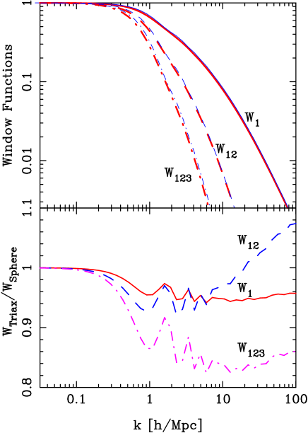
Figure 1: The triaxial halo window functions compared with the equivalent spherical halo window functions. In the top panel, thick lines represent triaxial haloes and thin lines spherical. Different line styles represent $W_{1}$, $W_{12}$ and $W_{123}$ as defined by equations (39), (43) and (44). The lower panel presents the ratio of the triaxial window functions to the spherical. The line styles are as in top panel.

Similarly, applying this procedure to the functions $W_{ij}$ and $W_{123}$, we find:

$$W_{ij}(M)\equiv\frac{(4\pi)^{2}}{8\pi^{2}}\int d{\bf a}\,p({\bf a}|M)\left(\frac{ab}{c^{2}}\right)^{2}\int d\alpha\,d(\cos\beta)\,d\gamma$$

$$\hskip 8.5359pt\times\prod_{\nu=\{i,j\}}\int dR_{\nu}R_{\nu}^{2}\,U(R_{\nu},M,{\bf a})\,{\rm j}_{0}[k_{\nu}R_{\nu}f(\theta_{k_{\nu}}^{\prime},\phi_{k_{\nu}}^{\prime})];$$ (43)

and

$$W_{123}(M)\equiv\frac{(4\pi)^{3}}{8\pi^{2}}\int d{\bf a}\,p({\bf a}|M)\left(\frac{ab}{c^{2}}\right)^{3}\int d\alpha\,d(\cos\beta)\,d\gamma$$

$$\hskip 8.5359pt\times\prod_{\nu=\{1,2,3\}}\int dR_{\nu}R_{\nu}^{2}\,U(R_{\nu},M,{\bf a}){\rm j}_{0}[k_{\nu}R_{\nu}f(\theta_{k_{\nu}}^{\prime},\phi_{k_{\nu}}^{\prime})].$$ (44)

In accordance with the set of conditions on the bispectrum, presented in Section 2.1, we see that the window functions, specified by equations (39), (43) and (44), are invariant under arbitrary rotations of the $k$ vector triple, and that they are also real functions of $k$.

As a point of practice for computing these functions, it is necessary to specify the initial coordinates of the $k$-vector triple. There is no loss of generality here, owing to the orientation average of the halo. We therefore choose ${\bf k}_{1}$ to be aligned with the $z$-axis of the reference coordinate system. The orientation of ${\bf k}_{2}$ is then specified in spherical polar coordinates so that the polar angle gives the angle between ${\bf k}_{1}$ and ${\bf k}_{2}$. The azimuthal angle of ${\bf k}_{2}$ is then, from equations (40) and (42), entirely arbitrary. Once ${\bf k}_{2}$ has been specified, ${\bf k}_{3}$ is then fixed through the triangle constraint. The window functions, and subsequently the bispectrum, then simply become functions of $|{\bf k}_{1}|$, $|{\bf k}_{2}|$ and the angle $\theta=\arccos\left({\bf k}_{1}\cdot{\bf k}_{2}/k_{1}k_{2}\right)$, as required for homogeneous and isotropic random fields.

Figure 1 shows a calculation of the window functions given by equations (39), (43) and (44) for equilateral triangle configurations, i.e $|{\bf k}_{1}|=|{\bf k}_{2}|=k$ and $\theta_{12}=2\pi/3$. In this calculation we have taken the ellipsoidal density profile to be the triaxial NFW model (see Section 4.1), and for illustration we have taken the joint axis ratio PDF to be simply the product of two delta functions: $p(a/c,b/c)=\delta^{D}\!(a/c-0.5)\,\delta^{D}\!(b/c-0.5)$. This constrains all haloes to take the form of prolate ellipsoids. The top panel shows the two usual characteristics: on large scales the window function approaches unity and on small scales it rapidly decays with oscillatory features present. To show the effect of halo triaxiality on these window functions in more detail, we compute the ratio of these quantities with the windows for the spherical model that result when $p(a/c,b/c)=\delta^{D}\!(a/c-1)\,\delta^{D}\!(b/c-1)$. The results of this are presented in the lower panel of the same figure. Clearly, the function $W_{123}$ is much more sensitive to the shape of the haloes than either $W_{1}$ or $W_{12}$. This leads us to conclude that the 1-Halo term becomes increasingly sensitive to the halo shape as the order of the clustering statistic increases.

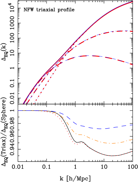
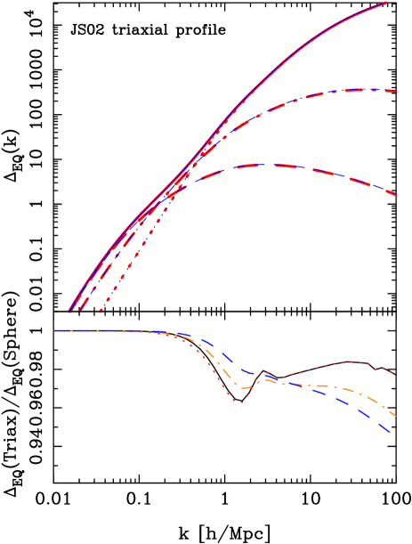
Figure 2: The equilateral bispectrum. Top panel presents the dimensionless bispectrum as defined in equation (46). Thick lines represent the triaxial haloes and thin lines the equivalent spherical haloes. The dot, dot-dash and dash lines represent the 1-, 2- and 3-Halo terms respectively and the solid lines represent the total. Bottom panel presents the ratio of the triaxial halo bispectrum to the spherical. The line styles are preserved, but note that the dotted line represents the ratio of the triaxial 1-Halo term to the spherical halo model 1-Halo term, similarly for the 2- and 3-Halo terms.

4 Results: Mass bispectrum

In this section we evaluate the bispectrum given by the summation of equations (26), (28) and (31), using our simplified expressions for the window functions given by equations (39), (43) and (44).

4.1 Computational details

We investigate two models for the halo profile $U(R,M,{\bf a})$: the first is a toy model that allows us to explore how modification of the halo shape alone affects the clustering – we refer to this as the ‘triaxial NFW’ model; the second is the more realistic density profile model of JS02, in which halo shape and central densities are not independent – we refer to this as the ‘JS02 model’. For a more thorough explanation of these we refer the reader to SW05 and JS02, respectively; note that in SW05 the triaxial NFW model is referred to as the ‘continuity model’. Common to both of these models is the density run, which is assumed to follow the NFW form

$$\rho(R)=\frac{\delta_{c}^{\rm triax}(M)\bar{\rho}}{y(1+y)^{2}};\,\hskip 28.45274pty\equiv R/R_{0}(M),$$ (45)

where $R$ is the ellipsoidal radial parameter from equation (12), $\delta_{c}^{\rm triax}(M)$ is the characteristic density of the halo and $R_{0}(M)$ is the scale radius; in the JS02 model these are treated as independent variables.

The PDF for the axis ratios, $p({\bf a}|M)$, is taken from JS02. We point out that in a recent paper, Lee, Jing & Suto (2005) valiantly attempted to derive the halo axis ratio PDF from the peak theory of Gaussian random fields. However, their predictions appear to be in conflict with the results from $N$-body simulations and so we do not consider their model further. We use the Sheth & Tormen (1999) mass function and halo bias functions, and correct for the different definitions of halo mass as discussed in SW05. In order to focus purely on the effects of triaxial modelling, we do not draw the concentration parameter from a probability distribution, as advocated by JS02, but treat it as a deterministic variable related to the halo mass.

Although in the previous section we greatly simplified our expressions for the halo window functions, we are still faced with the challenge of performing 7-D numerical integrals to compute the bispectrum. Evaluation of these expressions through a set of serial quadratures is unfeasible on a standard workstation. Instead, we advocate the use of an efficient multi-dimensional algorithm, such as the Korobov-Conroy (Korobov, 1963; Conroy, 1967) or Sag-Szekeres algorithm (Sag & Szekeres, 1964). However, the integrals over the ellipsoidal radial parameter $R$ require more care, due to the oscillatory nature of the integrand. To evaluate these we therefore employ a 1-D adaptive routine. Thus, for example, to evaluate the 1-Halo contribution to the bispectrum for a given $k$-space triangle (equation 26), we compute a 6-D numerical integral of a function that is itself the product of three 1-D integrals. Such numerical computations are achievable on a modern PC in a reasonable time frame. In Section 4.6 we present an independent determination of the triaxial halo model bispectrum, obtained through direct measurement from synthetic halo simulations. This provides a robust test of the veracity of the results produced by the multi-dimensional integrators.

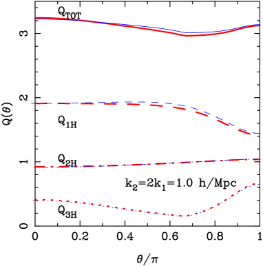
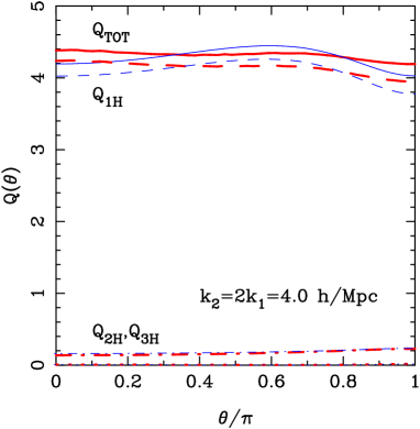
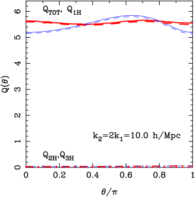
Figure 3: Reduced bispectrum $Q$ as a function of $\cos\theta\equiv{\bf k}_{1}\cdot{\bf k}_{2}/k_{1}k_{2}$, where $Q$ is defined through equation (47) and where we have considered the particular triangle configuration $|k_{2}|=2|k_{1}|$. The six panels show how the $Q$–$\theta$ curves evolve from large linear scales to small nonlinear scales; the sequence is shown for $k_{2}=(0.2,1.0,4.0,10.0)\,h\,{\rm Mpc}^{-1}$. Thick lines show the predictions of the triaxial halo model, thin lines are those for spherical haloes.

4.2 Equilateral triangles

Figure 2 (top panels) shows the predictions for the dimensionless bispectrum for equilateral triangles and for the triaxial NFW and JS02 models. This is defined as

$$\Delta_{\rm EQ}(k)=\frac{4\pi}{(2\pi)^{3}}k^{3}\sqrt{B_{\rm EQ}(k)}\ ,$$ (46)

where $B_{\rm EQ}(k)$ is the bispectrum for equilateral triangles. In addition to results for triaxial haloes (thick solid lines), we also show the results for spherical haloes (thin lines). The spherical halo model predictions are obtained by setting the axis ratio PDF to be a product of delta functions as discussed in Section 3.3. It is evident that deviations from the spherical halo model appear to be very small for both profiles. In the bottom panels of Figure 2, we illustrate the differences more clearly by plotting the ratio $\Delta^{2}_{\rm eq}({\rm triaxial})/\Delta^{2}_{\rm eq}({\rm spherical)}$ for the 1-, 2- and 3-Halo term, and their sum, respectively. As may be expected from the window functions, it is clear that the biggest departure from the spherical model occurs in the 1-Halo term, which is at most $\sim$ 7%. The 2- and 3-Halo terms also deviate by several percent, though only on scales below which their contribution to the total bispectrum is insignificant. On larger scales there is no appreciable difference from the spherical model. Thus, for the purposes of halo model calculations that wish to measure the equilateral triangle bispectrum, it is a good approximation to neglect the halo shape information in the 2- and 3-Halo terms. However, if one wishes to be accurate to the level of $\sim 5\%$ one must include shape information on the 1-Halo term.

On the other hand, it is now clear that the discrepancies ($\sim 50\%$) between the measurements of the equilateral triangle bispectrum from numerical simulations and the predictions for the halo model, noted in the work of SSHJ and Fosalba, Pan & Szapudi (2005), can not solely be attributed to the break down of the spherical halo approximation.

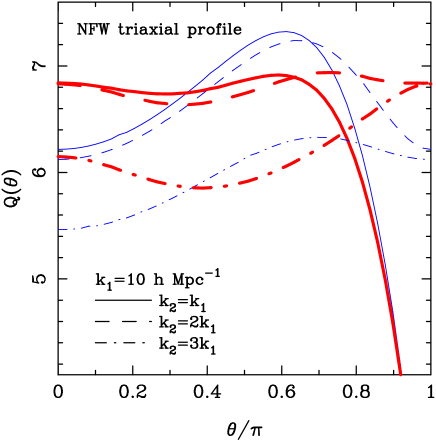
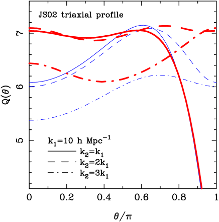
Figure 4: Dependence of $Q(\theta)$ on the ratio $k_{2}/k_{1}$. Thick lines represent the triaxial halo model predictions and thin lines denote the spherical model. Solid, dash and dot-dash lines represent the cases where the triangle configurations: $k_{2}=k_{1}$; $k_{2}=2k_{1}$; $k_{2}=3k_{1}$.

4.3 Variation with triangle configuration

We next consider the dependence of the bispectrum on the configuration of Fourier space triangles. This is achieved by fixing the lengths of $k_{1}$ and $k_{2}$ and then varying the angle between them. Since the effects caused by halo triaxiality are relatively small, we choose to examine the more sensitive reduced bispectrum, or hierarchical amplitude:

$$Q_{123}\equiv\frac{B_{123}}{P(k_{1})P(k_{2})+P(k_{2})P(k_{3})+P(k_{3})P(k_{1})},$$ (47)

where, for the case of the triaxial model predictions, $P(k)$ is the triaxial halo model power spectrum (SW05). In Figure 3 we show the results for the triaxial NFW profile model on various scales. In all four panels we have taken one of the fixed sides of the triangle to be twice the length of the other fixed side: $k_{2}=2k_{1}$. The four panels show the results for the case where $k_{2}=(0.2,1.0,4.0,10.0)\,h\,{\rm Mpc}^{-1}$.

The generic features of these curves have been examined in great detail in previous studies (Scoccimarro et al. 1998; SSHJ; Hou et al. 2005; Fosalba, Pan & Szapudi 2005). On large scales, it has been suggested that the variation in the configuration dependence can be attributed to coherent filamentary structures in the density field enhancing the contribution to $Q$ from collinear triangles (Scoccimarro et al., 1998). On intermediate scales, the density field begins to be dominated by collapsing objects that have almost isotropic spatial distributions, thus $Q$ shows much reduced variation across the configuration. Finally, on small scales, $Q$ is completely determined by the structure and shapes of the dark matter haloes. This overall evolution is well reproduced in our Figure 3.

Considering the relative differences between the triaxial and spherical predictions in Fig. 3, we make the following observations: on large scales ($k_{2}=0.2\,h\,{\rm Mpc}^{-1}$; top left panel), where $Q$ is dominated by the 3-Halo term, the affect of halo triaxiality is insignificant. This can easily be understood through considering the $k\rightarrow 0$ limit of equation (39); On intermediate scales ($k_{2}=1\,h\,{\rm Mpc}^{-1}$; top right panel), the magnitudes of the 1-, 2- and 3-Halo terms are comparable and one sees that there is a very small relative difference between the spherical and triaxial halo model predictions. This difference originates from the growing 1-Halo term, there being no perceivable variations in the 2- or 3-Halo terms; On smaller scales (lower panels), $Q$ is completely dominated by the 1-Halo term, and we see that there is a significant difference between the spherical and triaxial halo model predictions. The variation in $Q$ across the set of triangle configurations, for the triaxial haloes, appears to be much flatter than the variation apparent in the spherical halo model. It should also be noted that the positions of the maxima and minima of $Q$ are shifted.

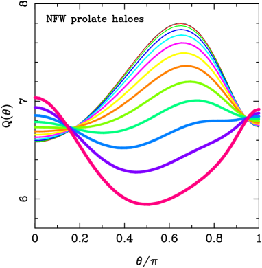
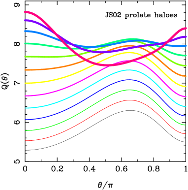
Figure 5: Dependence of $Q(\theta)$ on halo prolaticity. The axis ratio PDF is taken to be a product of delta functions. Increasing line thickness corresponds to increasing halo prolaticity, with the thinest line being $a/c=b/c=1.0$ and the thickest being $a/c=b/c=0.4$.

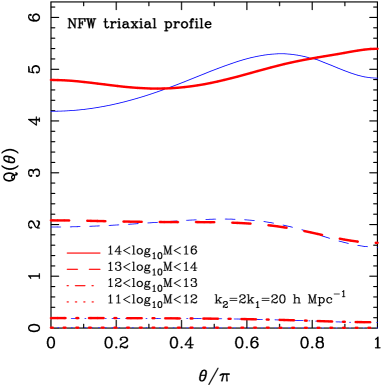
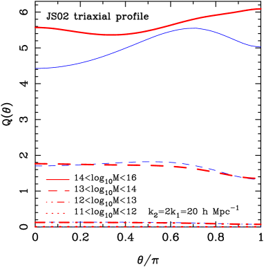
Figure 6: Dependence of $Q(\theta)$ on halo mass. Again, thick lines represent triaxial model predictions thin lines spherical.

In Figure 4 we investigate these apparent differences between the spherical and triaxial halo model in closer detail. Fixing $k_{1}=10\,h\,{\rm Mpc}^{-1}$, we consider the cases where $k_{2}/k_{1}=(1,2,3)$. Further, since the 1-Halo term dominates these scales, we focus in on the region over which it varies and ignore all other terms. In all cases we see that the triaxial model predictions for $Q$, for both density profile models, are suppressed with respect to the spherical model on angular scales where the $k$-vectors are close to equilateral triangles, and amplified on scales where the $k$-vectors are colinear and nonvanishing. Most importantly, from the figures it is clear that the overall functional forms exhibited by the predictions depend little on the density profile model, modulo an amplitude shift, and that it is the shape of the haloes that dictates the shape of the curves.

In the work of SSHJ, it was demonstrated that on small scales the predictions for the spherical halo model for $Q(\theta)$ exhibited a convex configuration dependence, whereas the measurements from N-body simulations showed a much flatter dependence with $\theta$. Indeed, SSHJ speculated that this disagreement was likely the result of a breakdown in the assumption of halo sphericity. More recently these discrepancies have been highlighted by the work of Fosalba, Pan & Szapudi (2005), who demonstrated that even with a somewhat ad-hoc modification of the halo boundaries, the configuration dependence on small scales can not be replicated in the spherical halo model. On contrasting these results with those above, we are lead to believe that the apparent discrepancies between theory and numerical simulation are likely attributed, in the main, to a break down in the spherical halo approximation. Moreover, it is highly unlikely that the exhibited configuration behaviour could be reproduced by other variations in the halo modelling prescription, e.g. through the stochasticity of the halo concentration parameter or through the inclusion of substructures. Such changes may alter the amplitude of $Q(\theta)$, as between the left and right panels of Figure 4, but they should not change the overall shape.

4.4 Dependence on halo shape

We now explore in closer detail how sensitive the triaxial halo model predictions are to the precise choice of the PDF for the axis ratios. This we do most directly by taking $p({\bf a}|M)$ as a product of Dirac delta functions (see Section 3.3). The sequence of curves in Figure 5 shows, in order of increasing thickness, the predictions for prolate dark matter haloes with axis ratios in the range $0.4\leq a/c=b/c\leq 1.0$, incremented in steps of $a/c=b/c=0.05$. Again we have set $k_{2}/k_{1}=2$ and $k_{1}=10\,h\,{\rm Mpc}^{-1}$. For both the triaxial NFW profile and the JS02 model a generic trend is apparent: for spherical haloes, the maximum in $Q(\theta)$ occurs for $\theta=2\pi/3$, with minima at $\theta=0$ and $\pi$. As haloes become more ellipsoidal the maxima in $Q(\theta)$ is strongly suppressed while the minima are enhanced. For the most prolate objects the maxima in $Q(\theta)$ lie at $\theta=0$ and $\pi$, while a deep minimum forms between $\theta=\pi/3$ and $2\pi/3$.

These trends can readily be understood by considering all possible placements of the $k$-space triangle within the Fourier transformed halo profile $U({\bf k}_{i},M,{\bf a},\mbox{\boldmath$\mathcal{E}$})$. Varying the configuration of the triangle, one sees that the largest contribution to the bispectrum will come from triangles that most optimally fill the halo volume in $k$-space. For a triaxial ellipsoid, its Fourier transform is also ellipsoidally symmetric. Thus, the ‘optimal’ triangle configuration is the one that matches most closely the halo’s symmetry. For spherical haloes this clearly means equilateral triangles (or close to); whereas for very ellipsoidal objects (e.g. the thickest lines in Fig. 5), the optimum configurations shift to those triangles where the $k$-vectors are coaligned. This explanation applies equally well to both the NFW and JS02 profiles since, by construction, they both share the same axis ratio PDFs. The apparent amplitude shifts in the JS02 predictions for $Q(\theta)$ are due to the fact that in this model, both the central density and concentration parameter depend on the halo axis ratios.

4.5 Dependence on halo mass

In the numerical simulation work of JS02 it was found that, for CDM models, the axis ratio PDF was conditional upon halo mass, and that more massive haloes were on average more triaxial than lower mass haloes. This can be understood from halo formation histories: high mass haloes form at late times in the Universe, whereas low mass haloes form at early times. Therefore, lower mass haloes have a longer period of time for particle orbits to undergo relaxation and become isotropic. Furthermore, since the haloes are assembled through the anisotropic accretion of lower mass haloes flowing along filaments, the halo shape at the time of formation will be more closely described as a triaxial ellipsoid. It is therefore of interest to consider how the bispectrum predictions depend on the abundances and masses of haloes.

Figure 6 shows the contribution to $Q(\theta)$ arising from four coarse bins in halo mass, for both the triaxial NFW and JS02 density profile models. Once again we set $k_{2}/k_{1}=2$ and $k_{2}=20h\,{\rm Mpc}^{-1}$. We take $P(k)$ in equation (47) as the power due to all halo masses, so that the sum of the contributions from the four bins equals the total $Q$. The main contribution to $Q$ comes from haloes with masses in the range $10^{14}h^{-1}M_{\sun}<M<10^{16}h^{-1}M_{\sun}$. We see that both the triaxial and spherical model predictions exhibit a ‘wave-like’ form with $\theta$. These waves are of similar amplitudes, but exhibit different ‘phases’. The maximum amplitude for the triaxial halo model predictions occurs at $\theta=\pi$, with a second peak of slightly lower amplitude at $\theta=0$, whereas for the spherical model, the peak amplitude is located at $\theta=2\pi/3$. These differences can be understood from the discussion surrounding Figure 5.

The next most significant contribution comes from haloes with masses in the range $10^{13}M_{\sun}h^{-1}<M<10^{14}M_{\sun}h^{-1}$. These curves show less of the wave-like form exhibited in the higher mass haloes. Crucially, however, for the case of the spherical haloes the maxima and minima in $Q$ occur at the same position as for the higher mass bin. For the triaxial predictions this is not the case, and the form of the curve has become almost consistent with that of the spherical halo model. This can be understood through the shifting of the mean of the JS02 halo axis ratio PDF to more spherical haloes as the halo mass decreases. Finally, one can now see how for the triaxial halo predictions the summation of the contributions to $Q$ from high and low mass haloes add de-constructively to give a relatively flat function across $\theta$ (cf. Fig. 3).

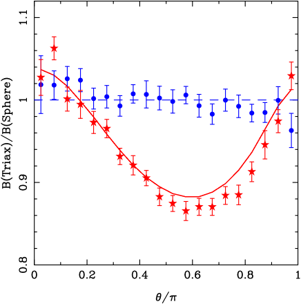
Figure 7: Test of the robustness of predictions of the triangle configuration dependent bispectrum. The star points show the mean bispectrum measured from an ensemble of 20 synthetic triaxial halo density fields ratioed to the predictions from the analytic spherical halo model. The circular points show the same, but for synthetic spherical halo density fields. The solid line shows the analytic predictions for the triaxial halo model.

4.6 Robustness of predictions

Owing to the relative obscurity of the high-dimensional integrators that we have used to solve the integrals in Section 3.2, we feel that it is necessary to demonstrate the robustness of their predictions. This we accomplish through the use of synthetic halo simulations. Following Peacock & Smith (2000) and Scoccimarro & Sheth (2002), we generate direct realizations of the triaxial halo density field through populating cubical regions of space with haloes that are sampled from the mass function, down to some limiting mass. Within each halo we then distribute equal mass particles in accordance with the required density structure, until the halo mass is reached. The spatial positions of the halo centres are chosen at random so that there is no large scale clustering of halos. From this particle distribution we then directly measure the bispectrum.

Figure 7 shows the measurement of the triaxial halo model and spherical halo model bispectrum in an ensemble of twenty synthetic simulations, ratioed with the analytic predictions of the spherical halo model. These are then compared with the numerically integrated predictions of our analytic results for the bispectrum 1-Halo term. We looked at triangles for which $k_{2}=2k_{1}=20h^{-1}$ Mpc. Clearly, the analytic predictions and direct measurements from the synthetic data are in excellent agreement (2$\sigma$ level). We are therefore confident that, for these problems, the integrators are accurate to at least $\sim 1\%$.

To summarize the main results of Section 4, we have convincingly demonstrated that the detailed shape of $Q(\theta)$ on small scales depends very sensitively on the shapes of dark matter haloes, and also their axis ratio PDF. Furthermore, we propose that the discrepancies observed between the theoretical predictions for $Q(\theta)$ and direct measurements from $N$-body simulations may be largely explained through the break down in the spherical halo approximation.

5 Galaxy clustering

We now turn our attention to the second of the questions posed in the introduction, and explore to what extent halo shapes impact on the galaxy clustering. Such information is of great importance if one wishes to use the halo model as a means for constraining the parameters of the HOD from observations.

5.1 Galaxies in the halo model

As a number of authors have shown, the halo model formalism can be extended to successfully model the clustering of galaxies (Seljak 2000; Peacock & Smith 2000; SSHJ; Berlind & Weinberg 2002, Yang et al. 2003, Cooray & Sheth 2003). The methodology follows ideas first laid down in earlier works by Neyman & Scott (1952) and others, but which are nicely summarized in Peebles (1980).

We note at the outset that one can write down the hierarchy of correlation functions directly from the mass clustering statistics by making use of the following simple substitutions. Firstly, we make the transformation

$$U({\bf r},M,{\bf a},\mbox{\boldmath$\mathcal{E}$})\rightarrow U_{g}({\bf r},M,{\bf a},\mbox{\boldmath$\mathcal{E}$})\equiv\frac{\rho_{g}({\bf r})}{\int d{\bf r}\rho_{g}({\bf r})}\ ,$$ (48)

where $U_{g}$ describes the average spatial distribution of galaxies within each halo normalized by the expected number of galaxies. Note that a sub- or superscript $g$ labels galaxy quantities. Secondly, instead of weighting the integrals over the halo mass function by mass, we weight by either the expected number of galaxies, or galaxy pairs, triplets etc., depending on whether we are considering the 3-, 2- or 1-Halo terms respectively. Thus we have

$$n(M)M \rightarrow n(M)\left<N|M\right>\ ,$$ (49)

$$n(M)M^{2} \rightarrow n(M)\left<N(N-1)|M\right>\ ,$$ (50)

$$n(M)M^{3} \rightarrow n(M)\left<N(N-1)(N-2)|M\right>\ ,$$ (51)

where

$$\left<N|M\right>=\sum_{N=1}^{\infty}N\,P(N|M)\ ,$$ (52)

$$\left<N(N-1)|M\right>=\sum_{N=2}^{\infty}N(N-1)\,P(N|M)\ ,$$ (53)

$$\left<N(N-1)(N-2)|M\right>=\sum_{N=3}^{\infty}N(N-1)(N-2)\,P(N|M)\ .$$ (54)

In the above equations $P(N|M)$ is the conditional halo occupation probability that gives the probability of finding $N$ galaxies in a halo of mass $M$. Lastly, in order to correctly normalize the clustering we perform the transformation

$$\bar{\rho}\rightarrow\bar{n}_{\rm g}=\int dM\,n(M)\left<N|M\right>\ ,$$ (55)

where $\bar{n}_{\rm g}$ is the mean number density of galaxies.

5.2 Galaxy correlation functions

Following the procedure described in the previous section, we can write down the two- and three-point correlation functions for the galaxies. Thus, for the two-point function, we find $\xi_{\rm g}$ to be:

$$\xi_{\rm g}=\xi^{\rm 1H}_{\rm g}+\xi^{\rm 2H}_{\rm g}\ ;$$ (56)

$$\xi^{\rm 1H}_{\rm g}=\frac{1}{\bar{n}_{\rm g}^{2}\,8\pi^{2}}\int dM\,d{\bf x}\,d{\bf a}\,d\mbox{\boldmath$\mathcal{E}$}\,n(M)\left<N(N-1)|M\right>p({\bf a}|M)$$

$$\hskip 28.45274pt\times\ \prod_{i=1}^{2}\left\{U_{\rm g}(M,{\bf r}_{i}-{\bf x},{\bf a},\mbox{\boldmath$\mathcal{E}$})\right\}\ ;$$ (57)

$$\xi^{\rm 2H}_{\rm g}=\frac{1}{(\bar{n}_{\rm g}\,8\pi^{2})^{2}}\int\prod_{i=1}^{2}\left\{dM_{i}\,d{\bf x}_{i}\,d{\bf a}_{i}\,d\mbox{\boldmath$\mathcal{E}$}_{i}\,n(M_{i})\,\left<N|M_{i}\right>\right.$$

$$\hskip 28.45274pt\times\,\left.p({\bf a}_{i}|M_{i})\,U_{\rm g}(M_{1},{\bf r}_{1}-{\bf x}_{1},{\bf a}_{1},\mbox{\boldmath$\mathcal{E}$}_{1})\right\}\xi^{s}_{2}(1,2)\ .$$ (58)

Similarly, we find $\zeta_{\rm g}$ to be:

$$\zeta_{\rm g}=\zeta^{\rm 1H}_{\rm g}+\zeta^{\rm 2H}_{\rm g}+\zeta^{\rm 3H}_{\rm g}\ ;$$ (59)

$$\zeta^{\rm 1H}_{\rm g}=\frac{1}{\bar{n}_{\rm g}^{3}8\pi^{2}}\int dM\,d{\bf x}\,d{\bf a}\,d\mbox{\boldmath$\mathcal{E}$}\,n(M)\left<N(N-1)(N-2)|M\right>$$

$$\hskip 28.45274pt\times p({\bf a}|M)\prod_{i=1}^{3}\left\{U_{\rm g}(M,{\bf r}_{i}-{\bf x},{\bf a},\mbox{\boldmath$\mathcal{E}$})\right\}\ ;$$ (60)

$$\zeta^{\rm 2H}_{\rm g}=\frac{1}{\bar{n}_{\rm g}^{3}(8\pi^{2})^{2}}\int\prod_{i=\{1,2\}}\left\{dM_{i}\;d{\bf x}_{i}\;d{\bf a}_{i}\;d\mbox{\boldmath$\mathcal{E}$}_{i}\;n(M_{i})p({\bf a}_{i}|M_{i})\right.$$

$$\hskip 28.45274pt\times\left.U({\bf x}_{i}-{\bf r}_{i},M_{i},{\bf a}_{i},\mbox{\boldmath$\mathcal{E}$}_{i})\right\}\left<N(N-1)|M_{1}\right>\left<N|M_{2}\right>\;$$

$$\hskip 28.45274pt\times U({\bf x}_{1}-{\bf r}_{3},M_{1},{\bf a}_{1},\mbox{\boldmath$\mathcal{E}$}_{1})\;\xi_{2}^{s}(1,2)+{\rm cyc}\ ;$$ (61)

$$\zeta^{\rm 3H}_{\rm g}=\frac{1}{(\bar{n}_{\rm g}8\pi^{2})^{3}}\int\prod_{i=1}^{3}\left\{dM_{i}\;d{\bf x}_{i}\;d{\bf a}_{i}\;d\mbox{\boldmath$\mathcal{E}$}_{i}\;\left<N|M_{i}\right>\,n(M_{i})\right.$$

$$\hskip 28.45274pt\times\,\left.p({\bf a}_{i}|M_{i})\,U({\bf x}_{i}-{\bf r}_{i},M_{i},{\bf a}_{i},\mbox{\boldmath$\mathcal{E}$}_{i})\right\}\,\zeta^{s}(1,2,3)\ .$$ (62)

5.3 Power spectrum & bispectrum

We next write down the power spectrum and the bispectrum. As for the analysis of the dark matter bispectrum, we define the useful functions $W^{\rm g}_{i}$, $W^{\rm g}_{ij}$ and $W^{\rm g}_{123}$ by applying the transformations described in Section 5.1 to equations (39), (43) and (44). Hence, the galaxy power spectrum can be written as:

$$P_{\rm g}=P^{\rm 1H}_{\rm g}+P^{\rm 2H}_{\rm g}\ ;$$ (63)

$$P^{\rm 1H}_{\rm g}=\frac{1}{\bar{n}_{\rm g}^{2}}\int dM\,\left<N(N-1)|M\right>n(M)\,W^{\rm g}_{12}(M)\ ;$$ (64)

$$P^{\rm 2H}_{\rm g}=\frac{P_{\,{\scriptscriptstyle{\rm L}}}}{\bar{n}_{\rm g}^{2}}\prod_{i=1}^{2}\int dM_{i}\,\left<N|M_{i}\right>n(M_{i})\,b(M_{i})\,W^{\rm g}_{i}(M_{i})\ .$$ (65)

Similarly, the galaxy bispectrum can be written as:

$$B^{\rm g}_{123}=B^{\rm g1H}_{123}+B^{\rm g2H}_{123}+B^{\rm g2H}_{123}\ ;$$ (66)

$$B^{\rm g1H}_{123}=\frac{1}{\bar{n}_{\rm g}^{3}}\int dM\,n(M)\left<N(N-1)(N-2)|M\right>$$

$$\hskip 28.45274pt\times\ W^{\rm g}_{123}(M)\ ;$$ (67)

$$B^{\rm g2H}_{123}=\frac{P_{\,{\scriptscriptstyle{\rm L}}}(k_{2})}{\bar{n}_{\rm g}^{3}}\int\!\!\!\prod_{i=\{1,2\}}\!\!\!\left\{dM_{i}\,n(M_{i})\,b(M_{i})\left<N(N-1)|M_{1}\right>\right\}$$

$$\hskip 28.45274pt\times\,\left<N|M_{2}\right>\,W^{\rm g}_{13}(M_{1})\,W^{\rm g}_{2}(M_{2})+{\rm cyc}\ ;$$ (68)

$$B^{\rm g3H}_{123}=\frac{1}{\bar{n}_{\rm g}^{3}}\int\prod_{i=1}^{3}\left\{dM_{i}\,\left<N|M_{i}\right>\,n(M_{i})\,W^{\rm g}_{i}(M_{i})\right\}$$

$$\hskip 28.45274pt\times\ B^{s}_{123}(M_{1},M_{2},M_{3})\ .$$ (69)

Owing to the fact that we are now modelling a discrete-point distribution, as opposed to a continuous field, we must apply corrections to both the power spectrum and bispectrum for shot noise. For this we follow SSHJ and use relations that have the same form as the Poisson case (Peebles, 1980):

$$P^{\rm g}_{c}(k)=P^{\rm g}(k)-\eta\ ;$$ (70)

$$B_{c123}^{g}=B^{g}_{123}-\eta[P^{g}_{c1}+P^{g}_{c2}+P^{g}_{c3}]-\eta^{2}\ ;$$ (71)

but where $\eta\equiv P^{g}(k\rightarrow\infty)$ instead of the usual $\eta=1/\bar{n}_{\rm g}$.

5.4 Central galaxy contribution

The above equations assume that the spatial distribution of the galaxies follows the underlying dark matter profile. We may also wish to impose the further constraint that, for every halo that contains at least one galaxy, a single galaxy lies at the halo centre of mass. In terms of the halo model this means that there will be a small modification to the clustering for terms that include the correlation of objects within the same halo. We now derive how this affects the small scale clustering.

Consider a triaxial halo of given mass $M$, with axis ratios ${\bf a}$, orientation $\mathcal{E}$ and with $N$ galaxies. For this halo we can identify one central object and $N-1$ satellites. For the two-point statistics, there will be $(N-1)(N-2)/2$ pairs of satellite galaxies and $N-1$ pairs that include the central galaxy and satellites. The two-point clustering of the satellite galaxies can be calculated as per usual. However, for the pairs that include the central galaxy, the clustering will be weighted by the density profile. This owes to the fact that the probability of finding a galaxy at position vector ${\bf r}$ from the central object now simply follows the density profile of galaxies. Hence, for the 1-Halo term in the power spectrum, we have the weight factor

$$\mathcal{W}_{12}^{2\rm g}(M,{\bf a},\mbox{\boldmath$\mathcal{E}$})=2!\sum_{N>1}P(N|M)\left\{(N-1)U_{g}({\bf k}_{1},M,{\bf a},\mbox{\boldmath$\mathcal{E}$})\right.$$

$$\hskip 14.22636pt\left.+\frac{1}{2}(N-1)(N-2)U_{g}({\bf k}_{1},M,{\bf a},\mbox{\boldmath$\mathcal{E}$})U_{g}^{*}({\bf k}_{2},M,{\bf a},\mbox{\boldmath$\mathcal{E}$})\right\}\ .$$ (72)

Note that the factor of $2!$ in the above expression arises since the term $U_{g}U_{g}^{*}$ is normalized by the total numbers of pairs with double counting. The galaxy window function is then obtained by averaging the weight factor $\mathcal{W}$ over the probability distribution for the axis ratios and the Euler angles: e.g. in general the $n$-point window function is given by

$$W^{g}_{12\dots n}(M)=\frac{1}{8\pi^{2}}\int d{\bf a}\,d\mbox{\boldmath$\mathcal{E}$}\,p({\bf a}|M)\mathcal{W}^{g}_{12\dots n}(M,{\bf a},\mbox{\boldmath$\mathcal{E}$})\ .$$ (73)

On computing the averages over $P(N|M)$ in equation (72), we obtain

$$\mathcal{W}^{\rm 2g}_{12}(M,{\bf a},\mbox{\boldmath$\mathcal{E}$})=\left<N(N-1)|M\right>|U_{g}({\bf k})|^{2}$$

$$\hskip 28.45274pt+2\,\left[\left<N-1|M\right>+P(0|M)\right]\left\{U_{g}({\bf k})-|U_{g}({\bf k})|^{2}\right\},$$ (74)

where we have suppressed the dependence of $U_{\rm g}$ on ${\bf a}$ and $\mathcal{E}$. The term $P(0|M)$, which is the probability of finding no galaxies in the halo, arises because the sum over galaxy numbers in equation (72) does not start from zero. Hence we have terms like

$$\sum_{N>1}(N-1)P(N|M)=\left<N-1|M\right>-P(0|M)\ .$$ (75)

On combining equations (63)-(65), (73) and (74), we arrive at a complete description of the galaxy power spectrum.

Similarly, for the bispectrum we will have $(N-1)(N-2)/2$ triplets that include the central galaxy and $(N-1)(N-2)(N-3)/3!$ triplets that comprise only satellite galaxies. The 2-Halo term in the bispectrum will be modified exactly as described for the power spectrum. However, for the 1-Halo term the weight factor must be modified as follows:

$$\mathcal{W}^{\rm 3g}_{123}(M,{\bf a},\mbox{\boldmath$\mathcal{E}$})=3!\sum_{N>2}P(N|M)\left\{\frac{1}{2}(N-1)(N-2)\prod_{i=1}^{2}U_{\rm g}({\bf k}_{i})\right.$$

$$\hskip 28.45274pt\left.+\frac{1}{6}(N-1)(N-2)(N-3)\prod_{i=1}^{3}U_{\rm g}({\bf k}_{i})\ \right\}\ ,$$ (76)

where we have included the factor of $3!$ to account for the fact that the profiles are normalized by the total triplets, which are counted in a way that does not prevent repetition. On computing the average over $P(N|M)$ we get

$$\mathcal{W}^{\rm 3g}_{123}(M,{\bf a},\mbox{\boldmath$\mathcal{E}$})=\left<N(N-1)(N-2)|M\right>\prod_{i=1}^{3}U_{\rm g}({\bf k}_{i})$$

$$\hskip 28.45274pt+\,3!\left\{\frac{1}{2}\left<N(N-1)\right>-\left<N-1|M\right>-P(0|M)\right\}$$

$$\hskip 28.45274pt\times\ \left[\prod_{i=1}^{2}U_{\rm g}({\bf k}_{i})-\prod_{i=1}^{3}U_{\rm g}({\bf k}_{i})\right]\ .$$ (77)

Thus on combining equations (66)–(69), (73) and (77) we also arrive at a complete analytic description of the galaxy bispectrum with one central galaxy and $N-1$ satellites.

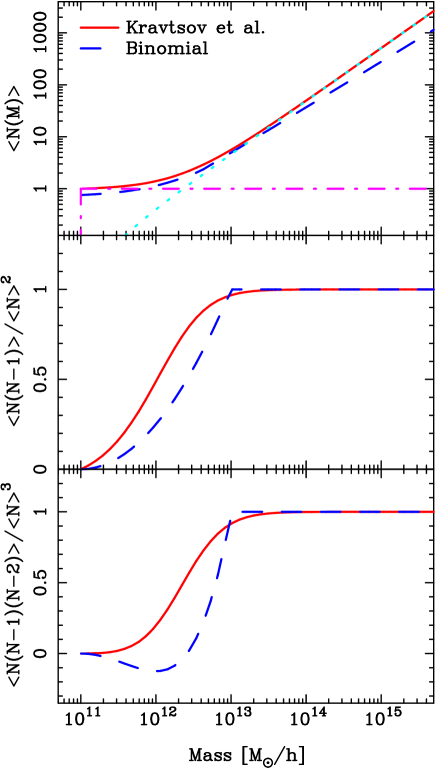
Figure 8: Comparison of the first three moments of the halo occupation probability function of K04, solid lines, with those of SSHJ, dashed lines. In the top panel, the dot-dash line represents the central galaxy contribution and the dotted line represents the satellite galaxy contribution.

5.5 Halo Occupation Distribution

To calculate the galaxy bispectrum we require a specific model for the mean spatial distribution of galaxies within each halo and also the first three moments of the halo occupation probability function. Firstly, we will make the usual assumption that the galaxy density distribution follows the mass profile, and hence $U_{g}({\bf r},M)\propto U({\bf r},M)$. In accordance with the ideas of the previous section, we will consider the effects on the bispectrum caused by placing one galaxy at the centre of each halo. Secondly, for $P(N|M)$, we will consider two potentially equally viable models from the literature: the first is the binomial model proposed by SSHJ, that was constrained to match the predictions of the semi-analytic models of Kauffmann et al. (1999); the second is the model developed by Kravtsov et al. (2004, hereafter K04). In this model it is assumed that if the halo mass lies above some minimum mass threshold, then there is always one central galaxy. The remaining $N-1$ galaxies are then taken to be satellites of the central galaxy, and it was found that these follow a Poisson process . The full details of both models are summarized in Appendix B.

In Figure 8 we show the differences between the first three factorial moments of the two probability functions. Note that in the limit of high masses, the power-law index of the first moment for the model of K04 is $\left<N\right>\propto M^{\alpha}$, with $\alpha\sim 1.0$, whereas for the binomial model it is $\alpha\sim 0.9$. In this limit the second and third factorial moments scale identically with the mean $\left<N\right>$ for both models. For halo masses below $\sim 10^{13}$ M_☉ (i.e. group and galaxy masses) the second and third moments are sub-Poisson in both models. Furthermore, for a given mass the binomial $P(N|M)$ is much narrower than for the K04 model.

5.6 Results: Galaxy Bispectrum

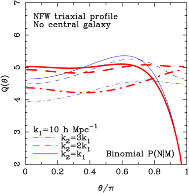
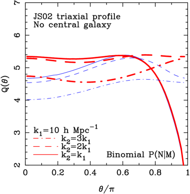
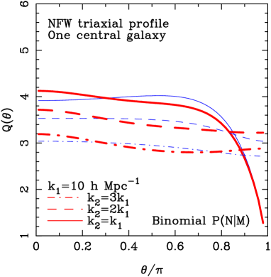
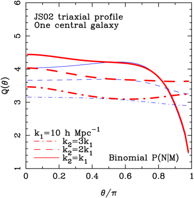
Figure 9: Configuration dependence of the galaxy bispectrum. The halo occupation probability function is taken to be the binomial model of SSHJ. Line styles are the same as in Figure 4.

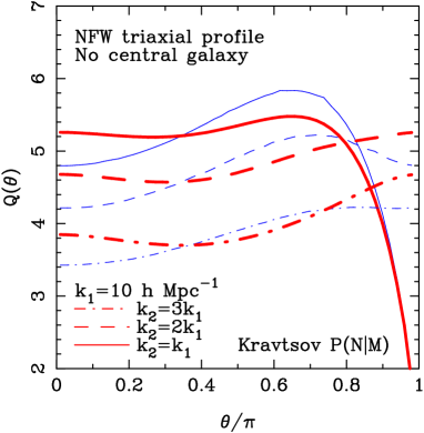
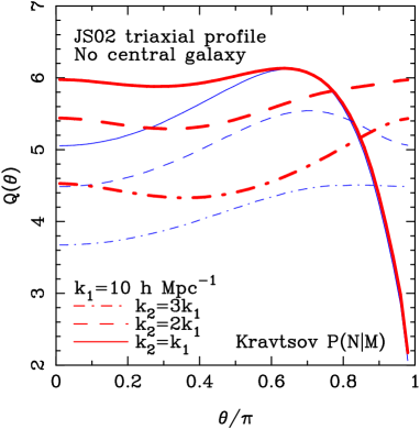
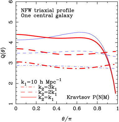
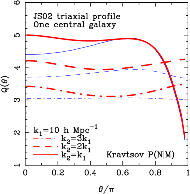
Figure 10: Same as Figure 9, however, this time the halo occupation probability function is taken to be the Poisson satellite model of K04. Again, line styles are the same as in Figure 4.

Figures 9 and 10 show the triaxial and spherical halo model predictions for $Q(\theta)$ for the binomial model of SSHJ and the Poisson satellite model of K04, respectively. In generating these predictions we chose the minimum halo mass for the binomial model to be $M_{\rm min}=10^{11}h^{-1}\ M_{\odot}$, which for the assumed cosmology gave a number density of galaxies $\bar{n}_{\rm g}=3.81475\times 10^{-2}h^{3}{\rm Mpc}^{-3}$. In order to compare the two occupation probability models consistently, it was important to remove any scaling due to the overall numbers of galaxies, since $Q\propto\bar{n}_{\rm g}$. This was done by finding the $M_{\rm min}$ in the K04 model that reproduced the same galaxy number density as for SSHJ. We found this to be $M_{\rm min}=1.28\times 10^{11}h^{-1}\ M_{\odot}$.

The top panels of both figures show the predictions for the case where all galaxies are distributed within the haloes according to the density profile (Section 5.3). The bottom panels show how the predictions change when one galaxy is assumed to be located at the centre of each halo (Section 5.4). As in Section 4 we show results for both the triaxial NFW profile (left panels) and the JS02 model (right panels). Once again, it is seen that the triaxial halo model predictions for $Q(\theta)$ differ quite substantially from those of the spherical model. The characteristic features of these predictions are essentially the same for all of the eight panels in the figures: the triaxial model produces a boosted signal for colinear triangle configurations and a suppression for configurations that are close to equilateral. However, and importantly, the functional form of these curves appears not to be strongly dependent on the precise form of the chosen HOD.

On comparison of these results with the mass bispectrum (Fig. 4), we see that the overall effect of triaxiality is weaker in the galaxy statistics. For the binomial model the effects are reduced by $\sim 50\%$, and for the model of K04 they are reduced by roughly $\sim 30\%$. The better sensitivity of the K04 model can be attributed to the fact that, for high mass haloes, the power-law index of the first moment of $P(N|M)$ is a steeper function of mass than the binomial model: as mentioned previously, $\alpha\sim 1$ for the K04 model and $\sim 0.9$ for the binomial model. In other words the most massive haloes, which are also the most triaxial, will host relatively more galaxies in the K04 model than in the binomial model.

Comparison of the upper and lower panels of Figures 9 and 10 reveals the overall importance of having one central galaxy. The first point to note is that, for both $P(N|M)$ models and density profiles considered, the overall effect is that $Q(\theta)$ is shifted by a factor $\sim 1$. After some tests, we found that this behaviour was a consequence of the bispectrum being normalized by products of the power spectrum (equation 47). To see this consider the following: on small scales, the power spectrum is more strongly weighted to contributions from low mass, low occupancy halos; this is due to the $\left<N(N-1)|M\right>$ weighting in the 1-Halo term. Whilst both the power spectrum and the bispectrum are sharply enhanced by the presence of the central galaxy, the power spectrum is relatively more enhanced owing to the added numbers of lower mass haloes that contribute to the signal; these are not included in the bispectrum as only haloes that host at least three galaxies can contribute. The result then follows.

Secondly, the central galaxy also appears to reduce the overall affect of halo triaxiality on the clustering. This can be understood by considering haloes that host three galaxies: when one is placed at the centre we find that the 1-Halo term is $B(k)\propto\left[U_{g}(k)\right]^{2}$ (equation 76), whereas for the case of no central galaxy, $B(k)\propto\left[U_{g}(k)\right]^{3}$. As was shown in Figure 1, the window functions become more sensitive to the halo shape as more points are placed in the $k$-space halo. Thus, placing one galaxy at the halo centre effectively removes one of these points.

As a final remark, we note that the combination of measurements for the triangle configurations with $k_{2}/k_{1}=1$, 2 and 3, in both the spherical and triaxial models, appear to depend strongly on the HOD. In particular, the spread in the amplitude of $Q$ as the ratio $k_{2}/k_{1}$ changes is substantially greater for the model of KS04, while the predictions for the SSHJ model appear closer to those of the mass bispectrum (cf Figure 4). The response of these predictions to the presence, or otherwise, of a central galaxy is also very different in the two models, with the SSHJ model being affected to a much greater extent by this assumption.

In summary, on small scales the reduced galaxy bispectrum has been shown to be a sensitive function of the halo shape and density structure, the occupation probability $P(N|M)$, and the central galaxy assumption. We note that the functional form of $Q(\theta)$ is most strongly affected by the shapes of the haloes themselves and is not greatly affected by the exact form of the HOD. However, the amplitude of each prediction, relative amplitudes of predictions made over different scales and the strength of the triaxiality effect are all sensitive to the particular choice of HOD.

6 Conclusions

In this paper we have explored how sensitive the real space bispectrum in cosmology is to the underlying shapes of dark matter haloes, for both matter fluctuations and galaxies. We achieved this through application of the triaxial halo model of SW05, adapting it to the problem of higher order statistics in a straightforward manner. In our model we accounted for dark matter haloes that have some known distribution of shapes and that are randomly orientated in space.

Analytic expressions were written down for the real space three-point matter correlation function and bispectrum. We then concentrated on the bispectrum and found that the 1-, 2- and 3-Halo terms could be compactly expressed as 7-D integral equations. These were solved numerically using an efficient multi-dimensional quadrature routine (Korobov, 1963; Conroy, 1967). Two models for the density profile of the triaxial haloes were considered: the first was the triaxial NFW model of SW05, which allowed us to explore the affects of halo shape alone on the bispectrum; the second was the more realistic model of JS02. The bispectrum was examined over a wide range of scales and for different configurations of $k$-space triangles.

We found that for equilateral triangle configurations the effect of halo triaxiality on the bispectrum was to produce a suppression on scales $k>0.2\,h\,{\rm Mpc}^{-1}$, relative to the spherical halo model predictions. This suppression was at the level of $<7\%$ for both density profiles. The reduced bispectrum was considered next, as function of $k$-space triangle configuration. We found that on large scales this quantity was insensitive to halo shapes. However, on small scales the predictions for the spherical and triaxial halo models differed significantly in both the amplitude and functional form of $Q(\theta)$. In general we found that, relative to the spherical model, the triaxial halo model predictions produced excess signal for triangle configurations that were colinear and non-vanishing, and a deficit for triangles that were close to equilateral. We observed that the overall form of $Q(\theta)$ depends little on the density profile model itself, modulo an amplitude shift, but rather that it is the shape of the haloes that dictates the shape of the curves.

Our results were then considered in relation to the discrepancies between the $N$-body simulations and the predictions from the spherical halo model that were noted by SSHJ and Fosalba, Pan & Szapudi (2005). We suggested that, for the case of the equilateral triangle configurations, the inconsistencies between theory and simulations are not due entirely to a break down in the spherical approximation. Rather, they are likely due to the combination of finite volume effects in the simulations and also other corrections to the halo model (SSHJ; Wang et al. 2004; Fosalba, Pan & Szapudi 2005). However, for the case of the configuration dependent bispectrum it was shown that the discrepancies could be well attributed to the break down of the spherical halo approximation, modulo an amplitude offset, which arises from the correction required to reconcile halo model predictions for the equilateral bispectrum with numerical simulations.

In the second part of this paper, we explored how halo shapes affect the real space galaxy bispectrum. Galaxies were included in the halo model in the usual way (Seljak 2000; SSHJ; Berlind & Weinberg 2002), and we considered two different schemes for the halo occupation probability function. The first of these was the binomial model developed by SSHJ, while the second was the Poisson satellite model of K04. For both probability functions, the predictions of the configuration dependent, reduced bispectrum were found to be very similar to those for the mass. However, the overall magnitude of the effect was reduced by $\sim 50\%$ for the binomial model, and $\sim 30\%$ for the K04 model. It was argued that the K04 model was more sensitive to halo shapes because of the stronger dependence on halo mass for the first moment of the occupation probability function. We also showed that the predictions for the binomial model possessed a stronger dependence on the presence of a central galaxy, when compared to the model of K04. Importantly, we found that the essential effects of triaxiality on the reduced bispectrum did not depend strongly on the exact details of the halo occupation distribution. However, a combination of measurements on different scales are sensitive to the both halo shape and the HOD.

We conclude that the bispectrum provides significant information about the shapes of dark matter haloes in addition to the (galaxy and mass) halo density profiles, and the halo occupation probability function. Consequently, in order to use the halo model to make precise constraints on the HOD, it will be necessary to take into careful consideration halo triaxiality. We remark, however, that our study did not account for the effect of redshift space distortions, which will have a significant impact on the behaviour of the galaxy bispectrum, particularly on small scales. Furthermore, we have also neglected the changes to the bispectrum that are caused by selecting different galaxy populations i.e., populations based on colour, luminosity or type. Neither have we considered realistic selection functions, or survey geometry. We reserve such investigations for future work, when we will study in more detail the bispectrum as a tool for measuring the HOD.

It remains to be seen whether measurements of the three-point statistics in weak lensing will be sensitive to halo shapes. An initial study of this problem has been conducted by Ho & White (2004), who calculated the three-point shear correlation function for triaxial haloes and found strong effects. The situation they considered was rather idealized, however, and was not a full halo-model calculation. Nevertheless, the potential for measuring such effects is clear. Recent work by Takada & Jain (2003b) showed, for an 11 square degree mock cosmic shear survey, that the three-point shear correlation function from ray-tracing simulations was in good agreement with the predictions of the spherical halo model. However, they noted that on small scales there were significant and unexplained discrepancies. For forthcoming weak lensing surveys which aim to cover even larger fractions of sky ($>100$ square degrees), the shear three-point functions will be accurately determined over a wide range of scales. Discrepancies between halo model predictions and observation will become very significant and important to understand. Moreover, the detection of shape information in the mass bispectrum or correlation function via weak lensing would be an important consistency test of the CDM paradigm, since it has been shown that plausible variants of the dark matter model, like SIDM and WDM, will give rise to a different spectrum of dark matter halo shapes (Avila-Reese et al., 2001; Yoshida et al., 2000).

Lastly, we mention that a recent study of the shapes of dark matter haloes in numerical simulations with gas cooling by Kazantzidis et al. (2004) has shown that the formation of central condensations may act to sphericalize the inner regions of haloes. At the virial radius, where halo shapes are usually measured, such processes will have relatively little effect. However, in order to achieve precise predictions to compare with observation, it will be necessary to quantify in detail how these effects modify halo profiles and axis ratio distributions.

Appendix A Rotation matrix

Owing to there being several equivalent ways to define the Euler angles for the rotation matrix ${\mathcal{R}}(\alpha,\beta,\gamma)$, we make explicit the definition that we use throughout. The matrix for the $z-y^{\prime}-z^{\prime\prime}$ rotation is given by:

$${\mathcal{R}}(\alpha,\beta,\gamma)\equiv\left(\begin{array}[]{ccc}\left(C_{\beta}\,C_{\alpha}C_{\gamma}\right.&\left(C_{\beta}\,S_{\alpha}\,C_{\gamma}\right.&-S_{\beta}\,C_{\gamma}\\ \left.-S_{\alpha}\,S_{\gamma}\right)&\left.+C_{\alpha}\,S_{\gamma}\right)&\\ \left(-C_{\beta}\,C_{\alpha}\,S_{\gamma}\right.&\left(-C_{\beta}\,S_{\alpha}\,S_{\gamma}\right.&S_{\beta}\,S_{\gamma}\\ \left.-S_{\alpha}\,C_{\gamma}\right)&\left.+C_{\alpha}\,C_{\gamma}\right)&\\ S_{\beta}\,C_{\alpha}&S_{\beta}\,S_{\alpha}&C_{\beta}\\ \end{array}\right)\ ,$$ (78)

where we have adopted the short hand notation $C_{x}=\cos x$ and $S_{x}=\sin x$.

Appendix B Occupation probability

B.1 Scoccimarro et al: binomial distribution

We now summarize the details of the occupation probability model proposed by SSHJ to describe the results from the semi-analytic galaxy formation models of Kauffmann et al. (1999). Sheth & Diaferio (2001) measured the first two moments of $P(N|M)$ from these models. For the first moment of they found

$$\left<N|M\right>=\left<N_{B}|M\right>+\left<N_{R}|M\right>:$$ (79)

$$\left<N_{B}|M\right>=0.7\left(\frac{M}{M_{B}}\right)^{\alpha_{B}}\ ;\hskip 14.22636pt\left<N_{R}|M\right>=\left(\frac{M}{M_{R}}\right)^{\alpha_{R}}\ ,$$ (80)

where $N_{B}$ and $N_{R}$ represent the numbers of red and blue galaxies. The blue galaxy parameters are $\alpha_{B}=0$ for haloes with masses in the range $10^{11}M_{\odot}h^{-1}<M<M_{B}$ and $\alpha_{B}=0.8$ for $M>M_{B}$, where $M_{B}=4.0\times 10^{12}M_{\odot}h^{-1}$. The red galaxy parameters are $\alpha_{R}=0.9$ and $M_{R}=2.5\times 10^{12}M_{\odot}h^{-1}$ for $M>10^{11}h^{-1}M_{\odot}$. For the second moment, they found that a sub-Poissonian distribution was preferred for low-mass haloes and an almost Poisson distribution for higher-mass haloes. They characterized this through

$$\left<N(N-1)|M\right>=\lambda^{2}(M)\left<N|M\right>^{2},$$ (81)

where the function $\lambda$ expresses the deviation from a Poisson probability distribution and has the form

$$\lambda(M)\approx\left\{\begin{array}[]{ll}\log_{10}(M/M_{11})^{1/2}&M\leq 10^{13}M_{\odot}\,h^{-1}\\ 1&M>10^{13}M_{\odot}\,h^{-1}\end{array}\right.$$ (82)

where $M_{11}\equiv 10^{11}M_{\odot}\,h^{-1}$.

SSHJ then proposed that, since $P(N|M)$ was not well described by a Poisson process, a better description might be afforded through the binomial distribution:

$$P(N=n|M)={\mathcal{C}}_{n}^{N_{M}}\,p_{M}^{n}(1-p_{M})^{N_{M}-n}\ ,$$ (83)

where ${\mathcal{C}}_{n}^{N_{M}}=N_{M}!/(N_{M}-n)!\,n!$. The binomial probability function is completely specified by two free parameters: the probability that out of one trial the event occurs $p_{M}\equiv p(M)$; and the total number of trials $N_{M}\equiv N^{\rm max}(M)$. These parameters were then fixed by matching the first and second moments to those measured from the semi-analytic galaxies. This gives

$$p_{M}=\left<N|M\right>\left[1-\lambda^{2}(M)\right]\ ,\hskip 14.22636ptN_{M}=\left[1-\lambda^{2}(m)\right]^{-1}.$$ (84)

Having specified $P(N|M)$ one may then calculate the galaxy clustering to any desired order. Of particular interest are the factorial moments. For the binomial distribution these are most readily obtained by differentiation of its frequency generating function:

$$\left<N(N-1)\dots(N-j)|M\right>\equiv\left.\frac{d^{j}F(t)}{dt^{j}}\right|_{t=0}$$

$$\hskip 56.9055pt=\left.\frac{d^{j}}{dt^{j}}\left\{p_{M}t+1-p_{M}\right\}^{N_{M}}\right|_{t=0}\ .$$ (85)

On performing the differentiation and substituting in for the relations (84), one finds the general relation (SSHJ)

$$\left<N(N-1)\dots(N-j)|M\right>=$$

$$\hskip 56.9055pt\lambda^{2}(2\lambda^{2}-1)\dots(j\lambda^{2}-j+1)\left<N|M\right>^{j+1}\ .$$ (86)

As a final remark we note that this particular occupation function is somewhat problematic to implement in practice: in order to sample from it, one requires that $N_{M}$ be an integer. In an analytic calculation this is not the case since one obtains the factorial moments directly from equation (86). Indeed, as $\lambda$ is a continuous variable, so to will be $N_{M}$. Thus when $N_{M}$ is small there are significant differences between the sampled and analytic distributions.

B.2 Kravtsov et al: central and satellite split

Much recent attention has focused on the separation of central and satellite galaxies, and characterizing the statistical properties of these objects as distinct populations (K04). The occupation probability under this prescription is therefore re-written

$$P(N|M)=\sum_{l=0}^{N}P_{\rm cent}(l|M)P_{\rm sat}(N-l|M)$$ (87)

where $P_{\rm cent}(l|M)$ and $P_{\rm sat}(N-l|M)$ are the probabilities for getting $l$ central galaxies and $N-l$ satellite galaxies, respectively.

In the work of K04 it was supposed that there was a one-to-one mapping between haloes (parent or substructure) and galaxies (central or satellite), and also that there was always only one central galaxy associated with the parent halo. This then lead to the following statement:

$$P_{\rm cent}(N=1|M)=\left\{\begin{array}[]{ll}1&\hskip 28.45274ptM\geq M_{\rm min}\\ 0&\hskip 28.45274ptM<M_{\rm min}.\end{array}\right.$$ (88)

Under this condition equation (87) simply becomes

$$P(N+1|M)=P_{\rm sat}(N)\ ;\hskip 28.45274ptM\geq M_{\rm min}\ .$$ (89)

Following this one may write down how the moments of the full halo occupation probability $P(N|M)$ are related to the moments of the satellite population $P_{\rm sat}(N|M)$.

K04 went on to show that the first moment of the satellite galaxy probability function was well characterized as a single power-law, $\left<N\right>_{\rm sat}\propto M$, with a steeper decline for lower halo masses. The exact function they found was

$$\left<N\right>_{\rm sat}=\left(\frac{M}{M_{1}}-C\right)^{\beta}\ ,$$ (90)

where $\beta=1.03$, $C\approx 0.045$ or $M_{1}/M_{\rm min}=22$, where $M_{\rm min}$ is the minimum halo mass. Furthermore, it was found that the second and third moments of the satellite galaxy distribution were well characterized by a Poisson process. Thus, the first three factorial moments of the full halo occupation probability function are:

$$\left<N\right>=\left<N_{s}\right>+1\ ;$$ (91)

$$\left<N(N-1)\right>=\left<N_{s}\right>^{2}-1\ ;$$ (92)

$$\left<N(N-1)(N-2)\right>=\left<N_{s}\right>^{3}-3\left<N_{s}\right>+2\ .$$ (93)

References

- Avila-Reese et al. (2001) Avila-Reese V., Col n P., Valenzuela O., D’Onghia E., Firmani C., 2001. ApJ, 559, 516
- Barnes & Efstathiou (1987) Barnes J., Efstathiou G., 1987. ApJ, 319, 575
- Bekenstein (2004) Bekenstein J.D., 2004. Phys. Rev. D, 70, 3509
- Benson et al. (2000) Benson A. J., Cole S., Frenk C. S., Baugh C. M., Lacey C. G., 2000. MNRAS, 311, 793
- Berlind & Weinberg (2002) Berlind A., Weinberg D., 2002. ApJ, 575, 587
- Bond & Myers (1996) Bond J. R., Myers S. T., 1996. ApJS, 103, 1
- Bullock et al. (2001) Bullock J. S., Kolatt T. S., Sigad Y., Somerville R. S., Kravtsov A. V., Klypin A. A., Primack J. R., Dekel A., 2001. MNRAS, 321, 559
- Chandrasekhar (1969) Chandrasekhar S., 1969. “Ellipsoidal figures of equilibrium“, Yale University Press, New Haven and London
- Conroy (1967) Conroy H., 1967. J. Chem. Phys., 47, 5307
- Cooray & Hu (2001) Cooray A., Hu W., 2001. ApJ, 554, 56
- Cooray & Sheth (2003) Cooray A., Sheth R. K., 2003. Physics Reports, 372, 1
- Dolney, Jain & Takada (2004) Dolney D., Jain B., Takada M., 2004. MNRAS, 352, 1019
- Efstathiou, Bond & White (1992) Efstathiou G., Bond J. R., White S. D. M., 1992. MNRAS, 258, 1
- Fosalba, Pan & Szapudi (2005) Fosalba P., Pan J., Szapudi I., 2005. astro-ph/0504305
- Frenk et al. (1988) Frenk C. S., White S. D. M., Davis M., Efstathiou G., 1988. ApJ, 327, 507
- Fry (1984) Fry J., 1984. ApJ, 279, 499
- Ghigna et al. (2000) Ghigna S., Moore B., Governato F., Lake G., Quinn T., Stadel J. 2000. ApJ, 544, 616
- Gnedin et al. (2004) Gnedin O., Kravtsov A., Klypin A., Nagai D., 2004. ApJ, 616, 16
- Ho & White (2004) Ho S., White M., 2004. ApJ, 607, 40
- Hou et al. (2005) Hou Y. H., Jing Y. P., Zhao D. H., B rner G., 2005. ApJ, 619, 667
- Jain & Bertschinger (1994) Jain B., Bertschinger E., 1994. ApJ, 431, 495
- Jenkins et al. (2001) Jenkins A., Frenk C. S., White S. D. M, Colberg J. M., Cole S., Evrard A. E., Yoshida N., 2001. MNRAS, 321, 372
- Jing & Suto (2002 – hereafter JS02) Jing Y. P., Suto Y., 2002. ApJ, 574, 538. (JS02)
- Kauffmann et al. (1999) Kauffmann G., Colberg J. M., Diaferio A., White S. D. M., MNRAS, 303, 188
- Kazantzidis et al. (2004) Kazantzidis S., Kravtsov A., Zentner A., Allgood B., Nagai D., Moore B., 2004. ApJ, 611, 73
- Klypin et al. (1999) Klypin A., Gottl ber S., Kravtsov A., Khokhlov A. M., 1999. ApJ, 516, 530
- Korobov (1963) Korobov N. M., 1963., “Number theoretic methods in approximate analysis”, Fizmatgiz, Moscow
- Kravtsov et al. (2004) Kravtsov A., Berlind A., Wechsler R., Klypin A., Gottlober S., Allgood B., Primack J., 2004. ApJ, 609, 35 (K04)
- Lee, Jing & Suto (2005) Lee J., Jing Y-P., Suto Y., 2005, astro-ph/0504623
- Ma & Fry (2000) Ma C., Fry J.N., 2000. ApJ, 543, 503
- Mathews & Walker (1970) Mathews J, Walker R. L., 1970. “Mathematical methods of physics”, W. A. Benjamin Publishers Inc., New York
- McClelland & Silk (1977) McClelland J., Silk J., 1977. ApJ, 217, 331
- Milgrom (1983) Milgrom M., 1983. ApJ, 270, 365
- Mo & White (1996) Mo H-J., White S. D. M., 1996. MNRAS, 282, 347
- Moore et al. (1999) Moore B., Quinn T., Governato F., Stadel J., Lake G., 1999. MNRAS, 310, 1147
- Navarro, Frenk & White (1997 – hereafter NFW) Navarro J. F., Frenk C. S., White S. D. M., 1997. ApJ, 490, 493 (NFW)
- Neyman & Scott (1952) Neyman J., Scott E. L., 1952. ApJ, 116, 144
- Peacock & Smith (2000) Peacock J. A., Smith R. E., 2000. MNRAS, 318, 1144
- Peebles (1980) Peebles P. J. E., 1980. “The Large-scale Structure of the Universe”, Princeton University Press, Princeton, New Jersey
- Power et al. (2003) Power C., Navarro J., Jenkins A., Frenk C. S., White S. D. M., Springel V., Stadel J., Quinn T., 2003. MNRAS, 338, 14
- Sag & Szekeres (1964) Sag T. W., Szekeres G., 1964. Math. Comput., 18, 254
- Scoccimarro et al. (1998) Scoccimarro R., Colombi S., Fry J. N., Frieman J. A., Hivon E., Melott A., 1998. ApJ, 496, 586
- Scoccimarro & Sheth (2002) Scoccimarro R., Sheth R. K., 2002. MNRAS, 329, 629
- Scoccimarro et al. (2001 – hereafter SSHJ) Scoccimarro R., Sheth R. K., Hui L., Jain B., 2001. ApJ, 546, 20. (SSHJ)
- Seljak (2000) Seljak U., 2000. MNRAS, 318, 203
- Sheth & Diaferio (2001) Sheth R. K., Diaferio A., 2001. MNRAS, 322, 901
- Sheth et al. (2001b) Sheth R. K., Diaferio A., Hui L., Scoccimarro R., 2001b, MNRAS, 326, 463
- Sheth et al. (2001a) Sheth R. K., Hui L., Diaferio A., Scoccimarro R., 2001a, MNRAS, 325, 1288
- Sheth & Jain (2003) Sheth R. K., Jain B., 2003. MNRAS, 345, 592
- Sheth & Tormen (1999) Sheth R. K., Tormen G., 1999. MNRAS, 308, 119.
- Smith & Watts (2005) Smith R. E., Watts P. I. R., 2005. MNRAS, 360, 203 (SW05)
- Spergel et al. (2003) Spergel D., & The WMAP team, 2003. ApJS, 148, 195
- Takada & Jain (2003a) Takada M., Jain B., 2003a. MNRAS, 340, 580
- Takada & Jain (2003b) Takada M., Jain B., 2003b. MNRAS, 344, 857
- Wang et al. (2004) Wang Y., Yang X., Mo H.-J., van den Bosch F., Chu Y., 2004. MNRAS, 353, 287
- Warren et al. (1992) Warren M. S., Quinn P. J., Salmon J. K., Zurek W. H., 1992. ApJ, 399, 405
- Yang, Mo & van den Bosch (2003) Yang X., Mo H.-J., van den Bosch F. C., 2003. MNRAS, 339, 1057
- Yoshida et al. (2000) Yoshida N., Springel V., White S. D. M., Tormen G., 2000. ApJ, 544, 87