Constraining the Evolutionary Stage of Class I Protostars: Multi-wavelength Observations and Modeling

Abstract

We present new Keck images at 0.9 $\mu$m and OVRO 1.3 mm continuum images of five Class I protostars in the Taurus star forming region. We analyze these data in conjunction with broadband spectral energy distributions and 8-13 $\mu$m spectra from the literature using a Monte Carlo radiative transfer code. By fitting models for the circumstellar dust distributions simultaneously to the scattered light images, millimeter continuum data, and the SEDs, we attempt to distinguish between flared disks, infalling envelopes with outflow cavities, and combinations of disks and envelopes. For each of these circumstellar density distributions, we generate grids of models for varying geometries, dust masses, and accretion rates, and determine the best fits by minimizing the residuals between model and data. Comparison of the residuals for best-fit disk, envelope, and disk+envelope models demonstrates that in general, models incorporating both massive envelopes and massive embedded disks fit the imaging+SED data best. The implied envelope infall rates for these disk+envelope models are generally consistent with infall rates derived by previous investigators, although they are approximately an order of magnitude larger than inner disk accretion rates inferred from recent spectroscopic measurements. In addition, the disk masses inferred from our models are close to or larger than the limit for gravitationally stable disks, indicating that Class I disks may undergo periodic episodes of enhanced accretion, perhaps as a result of gravitational instabilities. An important caveat to these results is that in some cases, no single model can fit all of the imaging and SED data well, suggesting that further refinements to models of the circumstellar dust distributions around Class I sources are necessary. We discuss several potential improvements to the models, as well as new constraints that will become available with upcoming millimeter and infrared facilities.

1 INTRODUCTION

The canonical picture of low-mass star formation is that of a rotating, collapsing cloud of dust and gas that forms a protostar surrounded by a disk (e.g., Terebey et al. 1984; Shu et al. 1987, 1993). Different stages of this theoretical evolutionary process have been equated with observed differences in the spectral energy distributions (SEDs) of protostellar objects, which have been grouped into classes 0-III based on their infrared spectral index and the ratio of sub-millimeter to bolometric luminosity (Lada & Wilking 1984; Lada 1987; Adams et al. 1987; André et al. 1993). In this classification scheme, Class 0 and I sources are still in the main accretion phase, and emit most of their radiation at far-IR and submm wavelengths due to reprocessing of light from the central protostars by dust grains in an infalling envelope. In contrast, Class II and III sources exhibit directly revealed pre-main-sequence stars in addition to emission from circumstellar disks.

This classification scheme is an attempt to represent discretely a continuous evolutionary sequence, and there are transition objects that create some blur between classes. Moreover, this sequence is defined solely from spatially unresolved SEDs, which contain only limited information about the circumstellar distributions. Thus, it is not clear that the observed differences in SEDs truly correspond to evolutionary changes in the circumstellar geometry. A crucial test is to constrain the geometry of material around members of these different evolutionary classes using spatially resolved images, and thereby either confirm or refute the evolutionary sequence inferred from spatially unresolved SEDs.

Direct imaging of Class II sources has shown that the bulk of the circumstellar material lies in disks (e.g., McCaughrean & O’Dell 1996; Koerner & Sargent 1995; Eisner et al. 2003, 2004), while there may be a small amount of material in tenuous envelopes (e.g., Grady et al. 1999; Semenov et al. 2004). Thus, Class II sources appear to be fully-assembled young stars surrounded by rotating disks from which they continue to accrete material. Direct images of the less evolved Class I sources are relatively rare, due to the large extinctions to these embedded objects, and thus the circumstellar geometry for these objects is not well constrained.

Studies of the emergent spectral energy distributions at wavelengths $\gtrsim 10$ $\mu$m have provided important, albeit ambiguous, constraints on the circumstellar dust distributions for Class I objects. Models incorporating infalling, rotating, envelopes with mass accretion rates on the order of $10^{-6}$ M_⊙ yr^-1 are consistent with observed SEDs (e.g., Adams et al. 1987; Kenyon et al. 1993a), and the compatibility of the derived mass accretion rates with statistically-inferred ages of Class I sources (Adams et al. 1987; Myers et al. 1987; Benson & Myers 1989; Kenyon et al. 1990) provides further support for these envelope models. However, for some objects whose SEDs can be explained by spherically-symmetric dust distributions, it has been suggested that nearly edge-on flared disk models may also be able to reproduce the observed SEDs (Chiang & Goldreich 1999). Observations that spatially resolve the circumstellar emission are necessary to remove the ambiguities inherent in SED-only modeling.

The circumstellar geometry is constrained directly by spatially resolved images. Scattered light at near-IR wavelengths (e.g., Kenyon et al. 1993b; Whitney et al. 1997, 2003b), with asymmetric emission morphologies observed in some sources, provides strong evidence that the circumstellar material is not spherically distributed around Class I objects. However, since scattered light traces tenuous dust in the surface layers of circumstellar dust distributions, it does not allow an unambiguous determination of geometry or other circumstellar properties. For example, while spherically-symmetric dust distributions can be ruled out, we show below that modeling of scattered light alone can not necessarily distinguish between a flattened envelope and a flared disk.

Modeling of images at multiple wavelengths can provide tighter constraints on geometry, since emission at different wavelengths arises in different layers of the circumstellar material, with short-wavelength scattered light from low-density surface layers and longer-wavelength emission from deeper, cooler layers at larger radii. For the Class I source L1551 IRS 5, spatially resolved observations at several wavelengths (e.g., Strom et al. 1976; Keene & Masson 1990; Butner et al. 1991; Lay et al. 1994; Ladd et al. 1995; Rodriguez et al. 1998; Chandler & Richer 2000; Motte & André 2001) and detailed spectroscopy (White et al. 2000) have been combined with SED modeling, providing important additional constraints on the models (Osorio et al. 2003). Moreover, the combination of low and high resolution millimeter observations facilitated distinction of compact disk emission and more extended envelope emission. Similar modeling of multi-wavelength observations for IRAS 04302+2247 provided firm constraints on the distribution of circumstellar material and the properties of the circumstellar dust grains (Wolf et al. 2003).

To further our understanding of the Class I population as a whole, we have obtained high spatial resolution observations of five additional Class I sources at multiple wavelengths which, when combined with SEDs, enable much tighter constraints on circumstellar dust models than available from any single dataset. We present images of scattered light at 0.9 $\mu$m and thermal emission from dust at 1.3 mm. In addition, we augment SEDs compiled from the literature with new photometry at 0.9 $\mu$m, 18 $\mu$m, 1.3 mm, and 3 mm wavelengths. Using the three dimensional radiative transfer code MC3D (Wolf & Henning 2000; Wolf 2003), we model our data in the context of three types of circumstellar dust distributions: 1) rotating infalling envelopes; 2) flared disks; and 3) combinations of envelopes+disks.

The best fits are obtained for models incorporating both an envelope and an embedded disk, although we show that pure disks or envelopes can reproduce certain aspects of our data. For each source, we discuss the properties of the best-fit models, including the geometry of the dust distributions and implied mass accretion rates. We use these results to help place Class I sources in the proper evolutionary context. Finally, we discuss refinements to the models that may improve agreement with observed multi-wavelength data, and describe new constraints that will become available from upcoming millimeter and infrared facilities.

2 OBSERVATIONS

2.1 The Sample

Our sample consists of five Class I sources in the Taurus star forming region drawn from the larger sample of protostars studied by Kenyon et al. (1993a). This subset was selected based on three criteria: 1) sources must be detected at red optical wavelengths ($F_{\rm 0.9\mu m}\gtrsim 10^{-5}$ Jy), 2) this emission must appear resolved, and 3) sources must emit strongly at millimeter wavelengths ($F_{\rm 1mm}\gtrsim 10^{-2}$ Jy). We initially observed the complete Kenyon et al. (1993a) sample at 0.9 $\mu$m with Keck/LRIS (see §2.3 and Appendix A), and chose only objects that satisfy our selection criteria for high angular resolution millimeter observations (§2.2) and detailed modeling. Our sample includes IRAS 04016+2610, IRAS 04108+2803B, IRAS 04239+2436, IRAS 04295+2251, and IRAS 04381+2540. General properties of our sample are discussed here, and information about individual objects is given below in §4.1.

The bolometric luminosities of our sample span 0.4 to 3.7 L_⊙, similar to the distribution of luminosities for the complete sample of Kenyon et al. (1993a), which has a median luminosity of 0.7 L_⊙. The SEDs for our sample objects are similar in shape, exhibiting high extinction of the central objects, small amounts of mid-IR absorption, and peaks near 100 $\mu$m. While these SED characteristics are common to most other sources in the Kenyon et al. (1993a) sample, several of the SEDs for their sample exhibit deep 10 $\mu$m absorption features. As discussed below, the depth of the 10 $\mu$m feature is correlated with source viewing angle; the dearth of objects with deep 10 $\mu$m absorption in our sample may therefore indicate selection against edge-on sources.

There are other clear selection effects for our sample, since we are biased toward sources exhibiting bright scattered light and millimeter continuum emission. For example, by selecting sources exhibiting bright scattered light nebulae, we are selecting against face-on sources where the directly visible, point-like protostar would dominate the short-wavelength emission, as well as objects with extremely high line-of-sight extinctions, such as one might expect for massive spherical envelopes. Since edge-on sources produce dimmer scattered nebulosity, these may also be under-represented in our sample. Finally, our selection criteria for bright millimeter emission favors objects with higher masses of dust concentrated in smaller volumes. Future observations of larger samples with more sensitive instruments are necessary to investigate these potential biases.

2.2 OVRO Observations

We imaged each source in our sample at both 1.3 mm (230 GHz) and 3 mm (115 GHz) with the OVRO Millimeter Array between 2002 August and December. The 3 mm observations were conducted in the “compact” array configuration, which provides baselines between 20 and 55 m, while the 1.3 mm observations were obtained mostly with the “equatorial” configuration, providing baselines from 30 to 120 m. For IRAS 04295+2251 and IRAS 04381+2540, 1.3 mm data were also obtained with the “high” configuration, which provides baselines from 35 to 240 m. Continuum data were recorded in four 1-GHz channels. We calibrated the amplitudes and phases of the data using quasars near on the sky ($\lesssim 20^{\circ}$) to our target sources. The flux of our target sources was calibrated using observations of Neptune and Uranus, which have known millimeter fluxes, to calibrate the response of the instrument. All data calibrations were performed using the OVRO software package MMA (Scoville et al. 1993). Using the calibrated data for each source, we inverted the interferometric visibilities to create an image, and de-convolved and CLEANed the images using the MIRIAD package (Sault et al. 1995). We averaged the data using robust weighting (with a robustness parameter of 0.5) to obtain a good balance between sensitivity and angular resolution.

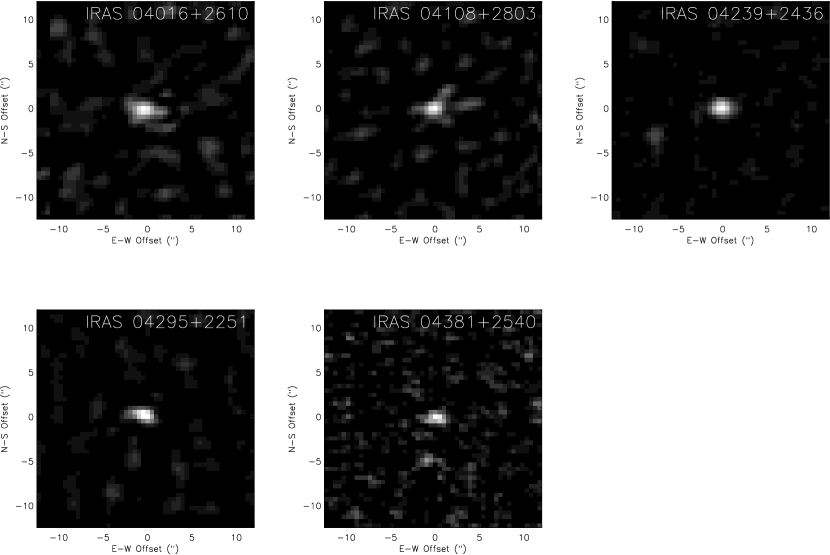
Figure 1: Images of our sample in thermal emission at 1.3 mm wavelength, obtained with OVRO. The origin of each image corresponds to the centroid of the millimeter emission. The J2000 coordinates at the origin of the images are (04${}^{\rm h}04^{\rm m}43\hbox to0.0pt{.\hss}^{\rm s}11$, +26${}^{\circ}18^{\prime}56\hbox to0.0pt{.\hss}^{\prime\prime}5$) for IRAS 04016+2610, (04${}^{\rm h}13^{\rm m}54\hbox to0.0pt{.\hss}^{\rm s}72$, +28${}^{\circ}11^{\prime}33\hbox to0.0pt{.\hss}^{\prime\prime}0$) for IRAS 04108+2803B, (04${}^{\rm h}26^{\rm m}56\hbox to0.0pt{.\hss}^{\rm s}29$, +24${}^{\circ}43^{\prime}35\hbox to0.0pt{.\hss}^{\prime\prime}1$) for IRAS 04239+2436, (04${}^{\rm h}32^{\rm m}32\hbox to0.0pt{.\hss}^{\rm s}06$, +22${}^{\circ}57^{\prime}26\hbox to0.0pt{.\hss}^{\prime\prime}3$) for IRAS 04295+2251, and (04${}^{\rm h}41^{\rm m}12\hbox to0.0pt{.\hss}^{\rm s}71$, +25${}^{\circ}46^{\prime}35\hbox to0.0pt{.\hss}^{\prime\prime}3$) for IRAS 04381+2540.

From our data, we measured photometric fluxes for our targets at both 3 mm and 1 mm wavelengths. The emission is much stronger at 1 mm, as expected for thermally-emitting dust, and thus the sources are more clearly detected at the shorter wavelength. In addition, since the angular resolution is inversely proportional to the observing wavelength, and because we obtained longer-baseline data at 1 mm than at 3 mm, our 1 mm images have better angular resolution. Our 1 mm images, shown in Figure 1, have angular resolution of $\sim 2^{\prime\prime}$, and rms sensitivity of $\sim 1.5-2.5$ mJy/beam. The measured fluxes, listed in Table A, are integrated over the OVRO beam, which is $\sim 2^{\prime\prime}$ at 1 mm, and $\sim 6^{\prime\prime}$ at 3 mm.

2.3 Keck/LRIS Observations

We obtained images of our Class I sample at 0.9 $\mu$m (Cousins $I$-band) using the W.M. Keck II telescope and the Low Resolution Imaging Spectrograph (LRIS; Oke et al. 1995) in imaging mode. The observations were conducted on 1998 October 30-31 and 1999 December 13. The integration time was 300 seconds, the seeing was $0\hbox to0.0pt{.\hss}^{\prime\prime}5-0\hbox to0.0pt{.\hss}^{\prime\prime}6$, the field of view was $6^{\prime}\times 8^{\prime}$, and the plate scale was 0.21 arcseconds per pixel. Image processing included bias subtraction and flat fielding. The photometric fluxes of the target sources, integrated over a $6\hbox to0.0pt{.\hss}^{\prime\prime}3$ (30 pixels) diameter aperture with background measured over an annulus extending from $26^{\prime\prime}$ to $30^{\prime\prime}$ (125-145 pixels), were calibrated using equatorial standards from Landolt (1992), assuming typical extinction coefficients for Mauna Kea (0.07 mag/airmass at $I$ band; Bèland et al. 1988); all sources were observed at an airmass of less than 1.1.

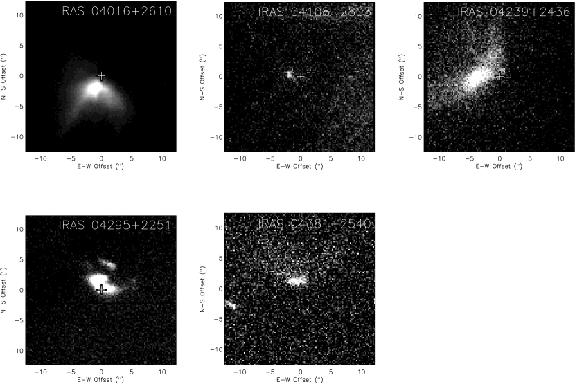
Figure 2: Images of our sample in scattered light emission at 0.9 $\mu$m wavelength, obtained with Keck/LRIS. The images are registered with respect to the centroid of the millimeter emission for each source (Figure 1), indicated by a cross.

All objects in our sample were detected at 0.9 $\mu$m, and show varying amounts of extended emission arising from scattered light due to dust-obscured central sources. Our images are shown in Figure 2. We determined absolute astrometry for these images by finding reference sources in common to our images and the 2MASS survey and computing a six coefficient fit for the image coordinates, plate scale, and distortion. The astrometry is accurate to $\sim 0\hbox to0.0pt{.\hss}^{\prime\prime}3$, including the uncertainty in our astrometric solution and the overall uncertainty from 2MASS.

Because we determine accurate positions for our $I$-band images, we can register the scattered light emission with the millimeter-wavelength emission observed with OVRO (§2.2). Since the longer wavelength radiation is optically thin, it traces dust mass and is therefore likely to be centered on the central source. In Figure 2, we have indicated the centroid of the millimeter continuum emission (and thus the likely position of the central protostar) with a cross. As we discuss below, the offset of the scattered light emission with respect to the central protostar provides valuable insights into source geometry and viewing angle.

2.4 Keck/LWS Observations

Our sources were also observed at 10.3 and 17.9 $\mu$m with the Keck Long Wavelength Spectrometer (LWS; Jones & Puetter 1993) between 1999 August and 2000 December. LWS allows diffraction-limited (FWHM=$0\hbox to0.0pt{.\hss}^{\prime\prime}2$) imaging over a $10^{\prime\prime}$ field of view, although the observations described here were obtained under poor seeing conditions, FWHM=$0\hbox to0.0pt{.\hss}^{\prime\prime}3-0\hbox to0.0pt{.\hss}^{\prime\prime}6$. With this seeing-limited resolution, none of our targets are angularly resolved at $10-18$ $\mu$m. Photometric fluxes were measured in a $1\hbox to0.0pt{.\hss}^{\prime\prime}92$ (24 pixels) diameter aperture, with subtraction of the sky background measured in an annulus spanning $4\hbox to0.0pt{.\hss}^{\prime\prime}0$-$6\hbox to0.0pt{.\hss}^{\prime\prime}4$ (50-80 pixels). Flat-fielding did not improve the data quality, and was therefore not applied before measuring photometry. Standard stars were observed each night to obtain atmospheric extinction curves, and curve-of-growth corrections were applied to each star to convert measured aperture photometry to infinite-aperture values. In addition, these Keck/LWS observations provided 8-13 $\mu$m spectra, which have been reduced and analyzed by Kessler-Silacci et al. (2005).

2.5 Spectral Energy Distributions

SEDs were constructed using photometric fluxes from the literature and new measurements at 0.9 $\mu$m (§2.3), 18 $\mu$m (§2.4), 1.3 mm, and 3 mm (§2.2). Uncertainties are not available for much of the photometry from the literature, and therefore we adopt estimated, uniform photometric uncertainties in the modeling described below (§3). Since these uniform error bars lead to the over-weighting of higher fluxes, we consider the logarithms of the SEDs in our modeling. The fluxes used in our analysis, converted into units of Jy, are listed in Table A and plotted along with best-fit models below in §4.

3 MODELING

We use the three dimensional Monte Carlo radiative transfer code MC3D (Wolf & Henning 2000; Wolf 2003) to model simultaneously the SEDs, 0.9 $\mu$m scattered light images, and millimeter continuum images of our sample of Class I sources (MC3D has been validated by benchmark comparison to other Monte Carlo and grid-based radiative transfer codes; Wolf et al. 1999; Pascucci et al. 2004). The basic model is that of a central emission source surrounded by obscuring dust of arbitrary geometry. The MC3D code solves the radiative transfer equation and determines the temperature distribution of circumstellar dust self-consistently. Moreover, the code takes into account absorption and multiple scattering events. The main inputs for this modeling are 1) parameters of the central star, 2) properties of dust grains, and 3) geometry of circumstellar dust. We now describe which properties in these categories are varied in our modeling, as well as our assumptions for other parameters.

Since our concern is primarily with understanding the geometry, we fix most of the stellar and dust parameters. For the models described below, we assume that the central object resembles a typical Class II T Tauri star. We therefore assume $T_{\ast}=4000$ K, $R_{\ast}=2$ R_⊙, and $M_{\ast}=0.5$ M_⊙ (e.g., Gullbring et al. 1998). Although few direct constraints exist on these parameters, spectroscopy of IRAS 04016+2610 has yielded an estimated effective temperature between $\sim 3300-4200$ K and a radius of $\sim 0.9$ R_⊙ (White & Hillenbrand 2004; Ishii et al. 2004), reasonably consistent with our assumptions. The dynamically-estimated stellar mass of IRAS 04381+2540 is $\sim 0.2-0.4$ M_⊙ (Brown & Chandler 1999), also compatible with our assumptions.

Accretion onto the stellar surface may generate substantial luminosity in shocks near the stellar surface, which would supplement the stellar luminosity (Calvet & Gullbring 1998; Gullbring et al. 2000): $L_{\rm central}=L_{\ast}+L_{\rm acc}$. In our modeling, we initially assume that $L_{\rm central}=L_{\ast}$, but we include a scale factor to allow for additional accretion luminosity (and/or slightly different stellar parameters from those assumed). As the last step in our modeling procedure, we find the value of $L_{\rm central}$ for which no scale factor is required. Although the spectral shape of emission from the accretion shock may differ from the stellar emission, we ignore this effect and assume that the temperature of all emission is 4000 K; the spectral shape is not critical given the extremely high optical depths in the inner regions of our models. In summary, all stellar parameters are constant from model to model, with the exception of a luminosity scaling that represents $L_{\rm acc}$.

We assume that the dust grains are spherical with a power-law size distribution $n(a)\propto a^{-3.5}$ (Mathis et al. 1977), where $a_{\rm min}=0.005$ $\mu$m and $a_{\rm max}=1.0$ $\mu$m, appropriate for ISM-like grains. We further assume that the dust is composed of a standard ISM mixture of 62.5% silicate and 25% ortho + 12.5% para graphite (e.g., Draine & Malhotra 1993; Weingartner & Draine 2001), with optical properties from Draine & Lee (1984). Previous authors have explored the effects of varying the chemical composition and particle size distribution of the circumstellar dust (e.g., D’Alessio et al. 1999, 2001). These parameters affect the overall SED, and 10 and 18 $\mu$m silicate features, to some extent. For simplicity, we keep the dust composition and particle size distribution fixed in our modeling.

The main remaining input for radiative transfer is the density distribution, and we focus our efforts on exploring the parameter space associated with circumstellar geometry. We consider three classes of models: rotating infalling envelopes, flared disks, and envelopes+disks. Each of these models is defined from an inner radius, $R_{\rm in}$, to an outer radius, $R_{\rm out}$. The inner radius is assumed to be 0.1 AU (comparable to the dust sublimation radius), although this parameter is not crucial to the modeling given the high optical depths near to the central protostar. However, $R_{\rm out}$ may have substantial effects on models for the circumstellar material, and thus we allow this parameter to vary in our modeling.

For each of the models considered in the following sections, several important parameters influence the density distributions, with concomitant effects on observed images and SEDs. In order to explore the effects of these parameters, we generate small grids of models by varying several important properties. Large grids are not possible due to the long run-time of Monte Carlo radiative transfer codes (typically several hours per model), and we therefore consider only three values for each parameter.

For the pure envelope model (§3.1), we vary the mass infall rate, $\dot{M}$, the centrifugal radius, $R_{\rm c}$, the outer radius, $R_{\rm out}$, and the inclination, $i$. The values of $\dot{M}$ are chosen to provide total envelope masses of $5\times 10^{-3},10^{-2},$ and $5\times 10^{-2}$ M_⊙; since the envelope mass depends to some extent on parameters other than $\dot{M}$ (see Equation 3 and §3.1), the accretion rates explored include 27 discrete values between $\sim 10^{-7}-10^{-4}$ M_⊙ yr^-1. Sampled values of the other parameters are $R_{\rm c}=30,100$, and $500$ AU; $R_{\rm out}=500,1000$, and $2000$ AU; and $i=5-90^{\circ}$ in increments of $5^{\circ}$. For the pure disk model, we vary the disk mass, scale height, outer radius, and inclination; $M_{\rm disk}=10^{-3},5\times 10^{-2},$ and $1.0$ M_⊙, $h_{0}=5,15$, and $25$ AU, $R_{\rm out}=500,1000$, and $2000$ AU, and $i=5-90^{\circ}$ in increments of $5^{\circ}$ . Finally, for the envelope+disk model, we assume $h_{0}=15$ AU, but allow $M_{\rm disk}$ to vary, in addition to varying several important envelope parameters: $\dot{M}$, $R_{\rm c}$, $R_{\rm out}$, and $i$. The range of envelope parameters are the same as for the pure envelope model, and we sample $M_{\rm disk}=10^{-3},10^{-2}$, and 1.0 M_⊙. All of the parameter values in these grids are chosen to bracket physically-plausible values.

In order to compare with our observations, we use MC3D to compute self-consistently the temperature distribution, the SED from 0.1-5000 $\mu$m, the scattered light image at 0.9 $\mu$m, and the dust continuum image at 1.3 mm, for each model. The best-fit models are determined by minimizing the residuals between model and data for the combined SED+imaging dataset. Specifically, we minimize the quantity

$$\chi_{\rm r,tot}^{2}\equiv\chi_{\rm r,SED}^{2}+\chi_{\rm r,0.9\mu m}^{2}+\chi_{\rm r,1mm}^{2}.$$ (1)

Here, $\chi_{\rm r,SED}^{2}$ is the reduced $\chi^{2}$ value of a model fitted only to the SED data, and $\chi_{\rm r,0.9\mu m}^{2}$ and $\chi_{\rm r,1mm}^{2}$ are the analogous quantities for the $I$-band and 1 mm images. Thus, $\chi^{2}_{\rm r,tot}$ gives equal weight to the three datasets (as opposed to a true $\chi_{\rm r}^{2}$ for the combined SED+imaging dataset, which would give more weight to the greater number of imaging datapoints relative to SED measurements).

To calculate $\chi_{\rm r}^{2}$ values for each dataset, we estimate the uncertainties by assuming that the best-fit model (amongst all classes of models considered) for a given dataset has a reduced $\chi^{2}$ value of unity, and setting the error bars accordingly. This means that when a model is fitted to a given dataset (e.g., SEDs), the reduced $\chi^{2}$ is given by the sum of the squared residuals divided by the minimum value of this quantity for all of the models considered: denoting summed squared residuals by $X^{2}$, $\chi_{\rm r}^{2}=X^{2}/{\rm min}(X^{2})$. Thus, Equation 1 can be re-written as

$$\chi^{2}_{\rm r,tot}=\frac{X^{2}_{\rm sed}}{{\rm min}(X^{2}_{\rm sed})}+\frac{X^{2}_{\rm 0.9\mu m}}{{\rm min}(X^{2}_{\rm 0.9\mu m})}+\frac{X^{2}_{\rm 1mm}}{{\rm min}(X^{2}_{\rm 1mm})}.$$ (2)

As mentioned above, when fitting the SED we minimize the difference between the logarithms of the model and data, to emphasize the shape of the SED over the peak value. In addition, we allow a scale factor between the model SED and the observed fluxes. When fitting 0.9 $\mu$m and 1 mm images, we first rotate the observed images to a position angle where the brightest scattered light is south of the millimeter emission, consistent with the position angle definition in our models.

Once the best-fit model out of these grids has been determined, we attempt to “zoom in” on the solution with more finely gridded values of inclination. During this zoom-in stage, we also vary $L_{\rm central}$ to produce the correct normalization between the modeled and observed SEDs (without a scale factor). Because the central luminosity is somewhat degenerate with the total optical depth of the system (e.g., Kenyon et al. 1993a), minor adjustments to $\dot{M}$ and/or $M_{\rm disk}$ may be required when $L_{\rm central}$ is varied. Thus, when zooming in on a solution, we vary $i$, $L_{\rm central}$, and $\dot{M}$ and/or $M_{\rm disk}$ simultaneously.

The effects of various parameters on the SEDs have already been explored by previous investigators (e.g., Adams et al. 1987; Kenyon et al. 1993a; D’Alessio et al. 1999), and some work has studied the effects on scattered light images (e.g., Whitney & Hartmann 1992; Whitney et al. 1997). We attempt to improve on this previous work by illustrating the effects of model parameters on our combined SED+imaging dataset for a broad range of circumstellar geometries, and discussing how degeneracies between fitted parameters can be broken. In the remainder of this section, we describe the rotating infalling envelope, flared disk, and disk+envelope geometries. In the following section, we present the best-fit model from each category for comparison to our observations.

3.1 Rotating, Infalling Envelope

The density distribution for a rotating, infalling envelope is given by (e.g., Ulrich 1976; Cassen & Moosman 1981; Terebey et al. 1984),

$$\rho_{\rm env}(r,\theta)=\frac{\dot{M}}{4\pi}(GM_{\ast}r^{3})^{-1/2}\left(1+\frac{\mu}{\mu_{0}}\right)^{-1/2}\left(\frac{\mu}{\mu_{0}}+2\mu_{0}^{2}\frac{R_{c}}{r}\right)^{-1}.$$ (3)

Here, $r$ is the radial coordinate, $M_{\ast}$ is the mass of the central star (assumed to be 0.5 M_⊙), $\dot{M}$ is the mass infall rate, $R_{c}$ is the centrifugal radius, $\mu=\cos\theta$ defines the angle above the midplane, and $\mu_{0}$ defines the initial streamline of the infalling material.

For each value of $r,\theta$, there is a unique value of $\mu_{0}$, since the streamlines of infalling particles do not cross. Before determining the density distribution using Equation 3, we analytically solve for $\mu_{0}$ :

$$\frac{r}{R_{c}}=\frac{\cos\theta_{0}\sin^{2}\theta_{0}}{\cos\theta_{0}-\cos\theta}=\frac{1-\mu_{0}^{2}}{1-\mu/\mu_{0}}.$$ (4)

This is a cubic equation with three solutions. The correct solution is the one for which $\sin\theta_{0}$ has the same sign as $\sin\theta$, and for which the solution is real. In other words, a particle that starts in the northern or southern hemisphere never leaves that hemisphere. The analytic solution is thus

$$\mu_{0}=\xi-\frac{1}{3\xi},$$ (5)

where $\xi$ is defined as

$$\xi\equiv\frac{\left(27\mu rR_{c}^{2}+\sqrt{729\mu^{2}r^{2}R_{c}^{4}+108R_{c}^{3}(r-R_{c})^{3}}\right)^{(1/3)}}{2^{(1/3)}3R_{c}}.$$ (6)

We include an outflow cavity in our envelope models by decreasing the density by some factor, $f_{\rm cav}$, in the polar regions of the circumstellar distributions. The cavity shape is defined by

$$\rho(r,z>z_{0}+r^{\zeta})=f_{\rm cav}\times\rho_{\rm env}(r,z).$$ (7)

Here, $z$ is the height above the midplane, $z_{0}$ describes how close to the star the outflow cavity begins, and $\zeta$ describes the opening angle and shape of the outflow. We fix $z_{0}=1$ AU, since this parameter does not have major affects on the observed SEDs or scattered light images. We also assume that within the outflow cavity, the density decreases by a factor of $f_{\rm cav}=4$ relative to the rest of the envelope; this value of $f_{\rm cav}$ produces the correct amount of extinction to match the observed short-wavelength SEDs. The cavity profile has some effect on the structure of modeled scattered light emission. However, these effects are small compared with the other envelope properties; thus, we fix the value of $\zeta$ at 1.1 in our analysis. Using other types of cavities (e.g., cones) may have small effects on the scattered light images, but will have negligible effects on SEDs (e.g., Whitney et al. 2003b).

We fit this envelope model to our data by varying $\dot{M}$, $R_{\rm c}$, the outer radius of the envelope, $R_{\rm out}$, and the viewing angle of the model, $i$. Some of these parameters produce degenerate effects on the models, which is why we generate grids where these parameters are varied simultaneously. However, we address the effects of each parameter below in order to shed light on how our different datasets constrain various envelope properties.

The accretion rate, $\dot{M}$, is one of the most important parameters in terms of its effects on the SED, since it is linked to the total envelope mass (Equation 3), and thus governs directly the optical depth of the dust surrounding the protostar (Figure 3). For higher mass accretion rates, the optical depth will increase, and less of the short-wavelength emission will escape (either directly or as scattered light). Moreover, the mid-IR absorption deepens, because of increased extinction of the stellar emission and absorption in the 10 and 18 $\mu$m silicate features. The short-wavelength radiation is re-processed and emitted at longer wavelengths, leading to more emission at far-IR through millimeter wavelengths for higher values of $\dot{M}$. The higher optical depths associated with large mass accretion rates also push the visible scattering surfaces outward, leading to somewhat larger $I$-band images. However, for very large accretion rates, the near-IR emission may be quenched altogether (Figure 3).

The centrifugal radius, $R_{\rm c}$, defines the radius in the model where material falling in from outer regions joins rotationally-supported material in the inner region. Outside of $R_{\rm c}$, the envelope is essentially spherical (except for the outflow cavity), while the density distribution is significantly flattened interior to the centrifugal radius. In addition, matter builds up at $R_{\rm c}$, leading to a region of enhanced density. For smaller values of $R_{\rm c}$, a larger fraction of the envelope material is spherically distributed, and the optical depth is larger for most sight-lines. Thus, models with small $R_{\rm c}$ show large near-IR extinctions and deep mid-IR absorption (largely degenerate with the effects of $\dot{M}$; Figures 3 and 4). In contrast, for larger $R_{\rm c}$, more of the envelope’s mass is relegated to the midplane, making it easier for emission to escape. Thus, scattered emission is stronger for larger values of $R_{\rm c}$. This parameter also has a critical effect on the modeled millimeter images: since the density is higher for radii $\lesssim R_{\rm c}$, the size of the millimeter emission will correlate with the centrifugal radius (Figure 4). Thus, the sizes of our millimeter images constrain $R_{\rm c}$ directly.

The outer radius also affects the model, mainly by changing the optical depth; larger values of $R_{\rm out}$ lead to more mass in the envelope, and thus more extinction of short wavelength light and more emission of long-wavelength radiation (Figure 5). Smaller values of $R_{\rm out}$ may require larger values of $\dot{M}$ and/or smaller values of $R_{\rm c}$ in order to correctly model the SED. $R_{\rm out}$ is constrained strongly from our scattered light and millimeter images, since larger outer radii produce larger images (Figure 5). For our sample, the observed sizes of scattered light constrain $R_{\rm out}$ to be $\gtrsim 1000$ AU, while the fact that the millimeter images are fairly compact rules out outer radii larger than $\sim 1500-2000$ AU.

Inclination is a crucial parameter for modeling both the SED and the scattered light images. As noted by previous authors (e.g., Kenyon et al. 1993a; Nakazato et al. 2003) and shown in Figure 6, the SED changes drastically depending on viewing angle. At larger inclinations, where the observer’s line of sight passes through more of the dense midplane, the overall optical depth of the model increases, leading to enhanced extinction at short wavelengths and absorption at mid-IR wavelengths. In contrast, for smaller inclinations the optical depth is lower, and for face-on models, the line of sight may go directly down the outflow cavity to the central protostar. In addition to affecting the amount of scattering or direct stellar radiation, the inclination also affects the shape of the scattered emission: for edge-on distributions, the scattered light arises mainly from the edges of the outflow cavity, producing a symmetric structure with two lobes. As the inclination decreases, one lobe brightens with respect to the other, and moves closer to the central protostar as the line of sight pierces further into the cavity. Finally, for inclinations close to face-on, the protostar is visible directly, swamping any scattered emission that might be present. Since our millimeter images are only marginally spatially resolved, inclination is not important in modeling this emission. However, the offset between 1 mm and 0.9 $\mu$m emission is sensitive to inclination; the visible scattering surface moves farther from the mass-sensitive millimeter emission for larger inclinations (Figure 6).

3.2 Flared Disk

The density distribution for a flared disk is given by (Shakura & Sunyaev 1973),

$$\rho_{\rm disk}(r,z)=\rho_{0}\left(\frac{R_{\ast}}{r}\right)^{\alpha}\exp\left\{-\frac{1}{2}\left[\frac{z}{h(r)}\right]^{2}\right\},$$ (8)

where

$$h(r)=h_{0}\left(\frac{r}{\rm 100\>AU}\right)^{\beta}.$$ (9)

Here, $r$ is the radial distance from the star in the disk mid-plane, $z$ is the vertical distance from the mid-plane, $R_{\ast}$ is the stellar radius, and $h$ is the disk scale height. We assume fixed values for the exponents of radial and vertical density distributions, $\alpha$ and $\beta$, respectively. For a flared disk in hydrostatic equilibrium, one expects $\beta=58/45$ (Chiang & Goldreich 1997), and we adopt this value. Using the relation that results from viscous accretion theory, $\alpha=3(\beta-1/2)$ (Shakura & Sunyaev 1973), we obtain $\alpha=2.37$. These values for $\alpha$ and $\beta$ are similar to those used in previous modeling of circumstellar disks (e.g., D’Alessio et al. 1999; Wood et al. 2002; Wolf et al. 2003). We fit the disk model to our data by varying M_disk, $h_{0}$, $R_{\rm out}$, and the viewing angle of the model, $i$.

The disk mass affects our modeled SEDs, scattered light images, and millimeter images. Regarding the SEDs, higher dust mass increases the optical depth, leading to higher obscuration of the central star, deeper 10 and 18 $\mu$m silicate absorption, and enhanced re-emission at long wavelengths. As illustrated by Figure 7, the disk mass also has substantial effects on the scattered light: for sufficiently small disk masses ($\lesssim 10^{-2}$ M_⊙) the central protostar is visible for inclination $\lesssim 70^{\circ}$ and this stellar radiation swamps any scattered light. However, for higher disk masses, the flared disk surface becomes sufficiently optically-thick to obscure the protostar, allowing scattered emission to be observed. The morphologies of millimeter images are only slightly affected by disk mass: more massive disks have millimeter emission detectable out to larger radii, leading to slightly larger observed images.

The effects of $h_{0}$ are similar to the effects of $M_{\rm disk}$ in some respects; however, SED+imaging data allows us to disentangle the two. Larger values of $h_{0}$ produce more absorption at short wavelengths, and if the scale height becomes large enough to obscure the central protostar, scattered emission becomes visible (Figure 8). These effects are similar to those produced by higher values of disk mass. However, the effects on the longer-wavelength emission differ; higher values of $h_{0}$ increase the far-IR flux, but have little effect on fluxes or image morphologies at millimeter wavelengths.

Changing $R_{\rm out}$ does not significantly affect the SEDs, as long as the disk mass is held fixed (Figure 9). This is because the optical depth of the model is not affected substantially by $R_{\rm out}$. However, there are small changes due to the larger surface area of optically-thick dust for larger values of $R_{\rm out}$. In addition, larger outer radii produce larger images in both scattered light and millimeter emission, since disk material is distributed to larger radii.

Disk viewing angle is a crucial property in modeling the SEDs and scattered light images (e.g., D’Alessio et al. 1999; Whitney & Hartmann 1992). Similar to the dependence of envelope model SEDs on inclination, more edge-on disk models exhibit deeper absorption at mid-IR wavelengths, and higher extinction of the central star (Figure 10). Inclination also substantially affects the observed scattered light: for moderate inclinations ($i\lesssim 55^{\circ}$), the central star is visible and dominates the $I$-band emission, while for larger inclinations the protostar is obscured and an asymmetric scattered light structure is observed. For nearly edge-on orientations, a symmetric, structure is observed, corresponding to the top and bottom surfaces of the flared disk. As for envelope models, our marginally resolved millimeter images can not constrain well the inclination, although the offset between scattered light and millimeter emission does probe the orientation of disk models.

3.3 Envelope+Disk

In addition to pure envelopes and pure disks, we consider a model incorporating both an envelope and an embedded disk. The main difference between this model and the pure envelope model is an enhanced density in the midplane, especially interior to the centrifugal radius. As a result of this enhanced midplane density, more long-wavelength emission is produced than for a pure envelope model. Since the amount of long-wavelength emission for a pure envelope model depends primarily on the mass infall rate, $\dot{M}$, additional long-wavelength emission from the disk component may allow good fits to the data with lower inferred values of $\dot{M}$. The effect of the disk component on the SED is illustrated in Figure 11.

In addition to larger fluxes, inclusion of a disk component also leads to more centrally concentrated modeled scattered light and millimeter images. With our marginally resolved millimeter images, we can not probe such density concentrations directly. However, as we discuss further below, comparison of our interferometrically measured fluxes, which trace compact emission, with lower-resolution measurements (e.g., Motte & André 2001; Young et al. 2003) can provide some constraint on the relative amounts of compact and large-scale material, providing an additional test of how well these models fit the data.

The envelope+disk model is implemented by computing the density distributions for both a disk and an envelope, and then setting the density of the combined model to be the greater of the two individual densities for a given position, $(r,\theta)$. The temperature distribution, spectral energy distribution, and images are then calculated self-consistently for the combined model using MC3D. In our current implementation of the disk+envelope density distribution, the outer radius of the disk cannot be specified independently of the outer radius of the envelope. Thus, our models may not truly represent a physical disk+envelope model, where one might expect the disk component to end at $R_{c}$. These models should therefore be regarded as only qualitative indicators that both disk and envelope components are needed to match the data.

3.4 Disk+Extinction Model

Finally, we consider another variation of a disk+envelope model, incorporating a flared disk density distribution plus foreground extinction. The extinction in this model mimics the obscuring nature of the envelope in the disk+envelope model described in §3.3, but employs a simpler geometry. In the following sections, we refer to this variation as a disk+extinction model.

We consider values of $A_{\rm V}$ ranging from 0 to 60 mag, which allows foreground extinctions much higher than expected from ambient material in the Taurus region (e.g., Kenyon & Hartmann 1995). Extinctions higher than possible from ambient cloud material ($A_{\rm V}\sim 5$) probably arise in material associated with the collapsing cloud cores surrounding the sources. Sub-millimeter fluxes observed in large-beam SCUBA maps (Young et al. 2003) can be used to estimate column densities, and thus extinctions toward our sample of Class I objects. Since higher extinctions are inferred for more compact dust distributions, models requiring larger values of $A_{\rm V}$ imply smaller dust structures. Based on the SCUBA fluxes (Young et al. 2003), extinctions larger than $\sim 5$ mag are only possible if the material is distributed primarily on scales smaller than $\sim 5000$ AU, on the order of expected envelope sizes.

In this disk+extinction model, the morphologies of scattered light and millimeter continuum images are unaffected by the uniformly-distributed obscuring envelope material, and thus the model images resemble those predicted by pure disk models. Since the dependence of the modeled images on various disk parameters is the same as for pure disk models (§3.2), we refer to Figures 7–10. However, the foreground extinction substantially alters the synthetic SEDs by eliminating much of the short-wavelength stellar flux observed for pure disks. This model thus provides a way to produce disk-like images at the same time as heavily reddened SEDs.

4 RESULTS

For each of the density distributions described in §3, we determine the model providing the best-fit to our combined SED+imaging dataset. The properties of the best-fit models, as well as the reduced $\chi^{2}$ residuals between models and data, are listed in Table 2, and the models are plotted in Figures 12–16. Our results clearly indicate that pure disk models are not applicable for our sample of Class I sources. Rather, the data suggest models incorporating a massive envelope with an outflow cavity, although most sources are fitted best by models including both envelopes and disks. In this section, we discuss general results of our SED and image fitting, then describe results for individual sources in detail in §4.1.

While the observed SEDs for our sample show fairly shallow absorption at mid-IR wavelengths (Figures 12–16), edge-on disk models produce deep mid-IR absorption (Figure 10; see also D’Alessio et al. 1999; Wood et al. 2002; Wolf et al. 2003), In addition, our asymmetric scattered light images rule out disk models close to edge-on, since such models would produce symmetric structures (Figure 10). However, the extended scattered light images indicate that disk models viewed close to face-on are not applicable either, since such models would be dominated by emission from the point-like central protostar. Since we observe spatially resolved, asymmetric scattered light toward our sample objects, we know that we are not directly observing the star, as would be the case for face-on or moderately inclined disk models.

Although there may be a narrow range of inclinations for which pure disk models can fit both the SEDs and scattered light images of some of our sources, substantial foreground extinction ($\gtrsim 20$ mag) is needed to make such a model consistent with the small optical/near-IR fluxes for our sample. As indicated by Table 2 and Figures 12–16, disk+extinction models provide far superior fits than pure disk models with $A_{V}=0$. However, the extinction values for the best-fit disk+extinction models are all much larger than expected from ambient material in the Taurus cloud (e.g., Kenyon & Hartmann 1995), indicating a large concentration of mass on small scales toward these Class I sources. Thus, the disk+extinction models imply the existence of massive envelopes in addition to disk components.

Pure envelope models also fail to fit the data well for most targets in our sample (Table 2). As illustrated in Figures 12–16, pure envelope models typically over-predict the peak flux in the SED. As discussed further below, pure envelopes also predict more extended millimeter emission than actually observed. Thus, pure envelope density distributions also do not seem suitable for explaining most features of the data for our sample.

For most, if not all, of the objects in our sample, the best fitting models (i.e., those for which the residuals between model and data are minimized) incorporate both an envelope and a disk (described either by disk+envelope or disk+extinction models; Table 2). However, while SEDs and 1 mm images are fitted best by disk+envelope models, the scattered light images for some sources seem to favor pure disk or pure envelope models. This may suggest that our disk+envelope model is too simplistic, and that a more complex implementation of disk+envelope models would allow all of the data to be fitted simultaneously. Alternately, the dust grain size distribution or composition may differ from our standard assumptions or vary radially or vertically within the model density distributions. One piece of evidence in support of the former hypothesis is the fact that the best-fit pure disk or envelope models, which usually fit the scattered light images well, generally have larger values of $R_{\rm out}$ than the best-fit disk+envelope models (Table 2). This suggests a flattened distribution of small dust grains that extends beyond the outer radius of our best-fit disk+envelope models. We discuss this issue further in §5.1.

One way to test the relative contributions of disks and envelopes is to compare the compact millimeter emission observed in our OVRO observations with more extended emission seen in lower-resolution single-dish observations (Motte & André 2001). As illustrated in the case of IRAS 04016+2610 in Figure 17, pure disks, pure envelopes, and disks+envelopes produce varying amounts of compact and extended emission, and thus comparison of high- and low-resolution millimeter data can help to distinguish between models. As described in §4.1, our interferometric fluxes typically (with one exception) differ by $\sim 20-50\%$ from the single-dish measurements of Motte & André (2001) (Table A), indicating that the sources we are observing produce most of their emission from compact inner regions. Thus, disks appear to be an important, if not dominant, component of the circumstellar distributions around our sample of Class I objects. Combined with the arguments presented above, this provides further evidence that the circumstellar material resides in some combination of disks and envelopes.

4.1 Results for Individual Sources

4.1.1 IRAS 04016+2610

IRAS 04016+2610 is an IRAS source (Beichman et al. 1986) lying at the western edge of the L1489 dark cloud (Benson & Myers 1989), and driving a molecular outflow (Myers et al. 1988; Terebey et al. 1989; Moriarty-Schieven et al. 1992). Previous modeling of this source in terms of an infalling envelope model found $\dot{M}\sim 5\times 10^{-6}$ M_⊙ yr^-1, $R_{\rm c}\sim 50$ AU, $i\sim 45-65^{\circ}$, and $L_{\ast}=3.72$ L_⊙ (Kenyon et al. 1993a; Whitney et al. 1997). An independent estimate of the inclination ($i\sim 60^{\circ}$) was obtained from observations of a compact molecular outflow (Hogerheijde et al. 1998). Previous observations of scattered light at near-IR wavelengths (Tamura et al. 1991; Whitney et al. 1997; Park & Kenyon 2002; Ishii et al. 2004) showed a similar morphology to our $I$ band observations. However, our observations enable for the first time accurate registration of the scattered light to the position of the central source, which allows better constraints on the circumstellar dust distribution than possible in previous analysis.

Our best-fit model for IRAS 04016+2610 incorporates both a rotating, infalling envelope and an embedded disk. This model fits all of our data well, including the 0.9 $\mu$m image, 1 mm image, and SED (Figure 12). The properties of this model are $\dot{M}=6\times 10^{-6}$ M_⊙ yr^-1, $R_{\rm c}=100$ AU, $R_{\rm out}=2000$ AU, and $M_{\rm disk}=0.01$ M_⊙. The properties of the envelope and disk components are consistent with previous analyses in the context of either model individually (Kenyon et al. 1993a; Whitney et al. 1997; Hogerheijde 2001).

In order to correctly fit the total luminosity of the system, we require a large central luminosity, $L_{\rm central}\approx 4.7$ L_⊙. This is substantially larger than the stellar luminosity inferred from near-IR spectroscopy (Ishii et al. 2004; White & Hillenbrand 2004), and suggests a large accretion luminosity. Since the total accretion rate determined from our fitting of disk+envelope models is not substantially higher than for other sources, we suggest that this additional luminosity may be generated in a more active accretion shock near the protostellar surface.

For IRAS 04016+2610, the flux measured in our $\sim 2^{\prime\prime}$ beam is approximately 40% of the value measured by Motte & André (2001) in an $11^{\prime\prime}$ beam. This is somewhat larger than the ratios predicted by our best-fit models, and may indicate that there is additional compact emission that we have not accounted for in the models. For example, if the disk is confined to radii smaller than $R_{\rm c}$, as opposed to $R_{\rm out}$ as assumed in our models, more mass would be concentrated at smaller radii. Finally, we note that although the pure envelope model appears to fit our combined imaging+SED dataset almost as well as the disk+envelope model (Table 2), the ratio of compact to extended emission for the pure envelope model is much smaller than observed, providing further support for the disk+envelope model.

4.1.2 IRAS 04108+2803B

IRAS 04108+2803 is a $22^{\prime\prime}$-separation binary system (e.g., Duchêne et al. 2004) in the L1495 region, and IRAS 04108+2803B is the component that appears less environmentally evolved based on its spectral energy distribution; it emits the vast majority of the far-IR emission from the system. IRAS 04108+2803B also shows large scatter in photometric observations, indicating that it may be a variable star (Kenyon et al. 1993a).

Previous modeling of this object in the context of infalling envelope models found $\dot{M}\sim 5\times 10^{-6}$ M_⊙ yr^-1, $R_{\rm c}\sim 70-100$ AU, $i\sim 30-60^{\circ}$, and $L_{\ast}=0.63$ L_⊙. (Kenyon et al. 1993a; Whitney et al. 1997). In contrast, Chiang & Goldreich (1999) showed that the SED of this object can be fit well by a flared disk model with $i=65^{\circ}$, $\beta=1.2$, and $R_{\rm out}=270$ AU. The small fractional polarization (5.1%) relative to other Class I sources ($\sim 20\%$; Whitney et al. 1997) was invoked as further evidence that the scattered emission from IRAS 04108+2803B arises in a disk rather than in the walls of an outflow cavity (Chiang & Goldreich 1999). Finally, IRAS 04108+2803B was modeled as a T Tauri star in a disk that is dynamically warped by a hypothetical stellar companion (Terquem & Bertout 1996).

Our results show that the data for this object cannot be fitted by a pure disk model, although the best fit is obtained for a model incorporating a massive disk in addition to an envelope (either disk+envelope of disk+extinction; Table 2; Figure 13). The best-fit disk+extinction model implies a disk with a mass of 0.6 M_⊙ surrounded by an envelope providing 25 mags of foreground extinction. The best-fit disk+envelope model for this source implies $\dot{M}=5\times 10^{-6}$ M_⊙ yr^-1, $R_{\rm c}=30$ AU, $R_{\rm out}$=500 AU, and $i=24^{\circ}$. The central luminosity is close to what one would expect for a T Tauri star, $L_{\rm central}\approx 0.4$ L_⊙. The disk mass of our best-fit model is 0.5 M_⊙ (Table 2); however, as discussed in §5.2, this is likely an over-estimate.

The ratio of compact to extended millimeter emission (0.7; Table A) implies that a large fraction of the flux is generated by a compact disk component. Thus, this source appears to be extremely disk-dominated, supporting the hypothesis of Chiang & Goldreich (1999). On the other hand, a massive envelope component also appears necessary to fit the imaging+SED data, consistent with previous models (e.g., Kenyon et al. 1993a) and recent Spitzer observations which attribute 15.2 $\mu$m CO₂ ice absorption to a cold envelope (Watson et al. 2004).

4.1.3 IRAS 04239+2436

IRAS 04239+2436 is an IRAS source (Beichman et al. 1986) with a bright scattered light nebula (Kenyon et al. 1993b), which has been tentatively associated with high-velocity molecular gas (Moriarty-Schieven et al. 1992). Previous modeling of SEDs and near-IR scattered light (separately) in the context of rotating, infalling envelopes, found $\dot{M}\sim 2-4\times 10^{-6}$ M_⊙ yr^-1, $R_{\rm c}\sim 10-70$ AU, $i=30-55^{\circ}$, and $L_{\ast}=1.23$ L_⊙ (Kenyon et al. 1993a; Whitney et al. 1997).

Although the SED for this source is fit best by a disk+envelope model, the combined dataset is fit comparably well by a disk+extinction model with $A_{V}=20$ (Table 2; Figure 14). Thus, while there seem to be both disk and envelope components, the exact density profile of the source may not be matched exactly by either the disk+envelope or disk+extinction models. As we discuss further in §5.1, the fact that the disk+envelope model fails to represent accurately our 0.9 $\mu$m image may suggest that an additional flattened distribution of small dust grains extending out to $\sim 2000$ AU (not currently included in the model) is necessary to fit all of the data simultaneously. Assuming that our best-fit disk+envelope model provides an accurate tracer of the mass, the properties of this source are $\dot{M}=3\times 10^{-6}$ M_⊙ yr^-1, $R_{\rm c}\sim 30$ AU, $R_{\rm out}=1000$ AU, $M_{\rm disk}=0.5$ M_⊙, $L_{\rm central}=1.5$ L_⊙, and $i=34^{\circ}$. However, as discussed in §5.2, this value of $M_{\rm disk}$ may be substantially over-estimated.

In addition to our modeling, there are several arguments suggesting that IRAS 04239+2436 is surrounded by both a massive envelope and an embedded disk. The ratio of compact to extended millimeter emission (Table A) shows that a pure envelope model cannot fit the data, and thus there must be a compact disk component. On the other hand, recent Spitzer observations find a deep 15.2 $\mu$m CO₂ ice absorption feature, which likely arises in a large, cold envelope (Watson et al. 2004). These arguments provide further support for a combined disk+envelope distribution of material around this source, and motivate future modeling that can fit all of the data simultaneously.

4.1.4 IRAS 04295+2251

IRAS 04295+2251 has appeared point-like in previous near-IR imaging observations (e.g., Park & Kenyon 2002), and is tentatively associated with a molecular outflow (Moriarty-Schieven et al. 1992). Previous investigators analyzed SEDs and scattered light images (separately) in the context of infalling envelope models, and found $\dot{M}=1-5\times 10^{-6}$ M_⊙ yr^-1, $R_{\rm c}=70-100$ AU, $i=0-30^{\circ}$, and $L_{\ast}=0.44$ L_⊙ (Kenyon et al. 1993a; Whitney et al. 1997). It has also been suggested that a pure disk model may be able to fit the SED for this source (Chiang & Goldreich 1999).

Our modeling shows that the best-fit is obtained for a density distribution including both envelope and disk components (Table 2; Figure 15). Formally, the best-fit is obtained for a disk+extinction model including a 1.0 $M_{\odot}$ disk surrounded by an envelope that provides 20 magnitudes of extinction. The disk+envelope model also provides a good fit to the data, and the properties of this model are $\dot{M}=4\times 10^{-6}$ M_⊙ yr^-1, $R_{\rm c}\sim 100$ AU, $R_{\rm out}=500$ AU, $M_{\rm disk}=1.0$ M_⊙, $L_{\rm central}=0.6$ L_⊙, and $i=22^{\circ}$. As for other sources in our sample, the inferred values of $M_{\rm disk}$ for best-fit models are probably too high (§5.2). The ratio of compact to extended millimeter emission observed for IRAS 04295+2251 (0.42; Table A) is consistent with that predicted for the best-fit disk+envelope model, and implies a relatively disk-dominated density distribution.

4.1.5 IRAS 04381+2540

IRAS 04381+2540 is in the B14 region, and is associated with high-velocity molecular gas (Terebey et al. 1989). In addition, extended near-IR emission has been observed toward this object (Tamura et al. 1991). Previous modeling in the context of a rotating, infalling envelope found $\dot{M}=5-13\times 10^{-6}$ M_⊙ yr^-1, $R_{\rm c}=50-300$ AU, $i=30-75^{\circ}$, and $L_{\ast}=0.66$ L_⊙ (Kenyon et al. 1993a; Whitney et al. 1997). Moreover, the inclination was estimated independently from observations of a compact molecular outflow to be $\sim 40-70^{\circ}$ (Chandler et al. 1996).

Our modeling shows that the best fit is obtained for a density distribution incorporating both an envelope and a disk (Table 2; Figure 16). The properties of the best-fit disk+envelope model are $\dot{M}=9\times 10^{-6}$ M_⊙ yr^-1, $R_{\rm c}=30$ AU, $M_{\rm disk}=1.0$ M_⊙, $i=38^{\circ}$, and $L_{\rm central}=0.6$ L_⊙. The disk+extinction model also provides a good fit, and may provide a more accurate representation of the 0.9 $\mu$m scattered light image. These results indicate that the circumstellar dust distribution around IRAS 04381+2540 is dominated by a disk, although a massive envelope is also required to fit the data. However, the values of $M_{\rm disk}$ in Table 2 are probably over-estimated (§5.2) and the disk mass may be closer to $\sim 0.2$ M_⊙ for this object.

A potential problem with the best-fit disk+envelope model is that it does not correctly reproduce the observed ratio of compact to extended millimeter flux (Table A). Rather, this ratio indicates that the density distribution for this source is envelope-dominated. This may indicate that there is envelope material distributed uniformly over large spatial scales, leading to large amounts of extended flux being resolved out in our OVRO image. This is consistent with an extended structure extending to large radii from the central source ($\gtrsim 3000$ AU) observed by Young et al. (2003), and may favor the disk+extinction model, which allows a large mass of dust to be distributed out to larger radii. Regardless of the exact density distribution, it seems that both disk and envelope components are necessary to fit the data for this source.

The high derived accretion rate for IRAS 04381+2540, as well as the strong indication from Table A that the source is envelope-dominated, suggest that this object may be evolutionarily younger than other sources in our sample. Moreover, the mass accretion rate may be underestimated for this source: the mass of this object has been estimated dynamically from millimeter spectral line observations to be $\sim 0.2-0.4$ M_⊙ (Brown & Chandler 1999), somewhat lower than our assumed value of 0.5 M_⊙, which implies that the value of $\dot{M}$ derived above may be underestimated by $\sim 10-30\%$ (Equation 3).

5 DISCUSSION

In §4, we fit our combined imaging+SED data for a sample of Class I sources with several models for the circumstellar dust distribution: flared disks, collapsing envelopes, and combinations of disks and envelopes. Of the models considered, disk+envelope (and/or disk+extinction) density distributions generally provide the smallest residuals between models and data (Table 2). The properties of best-fit models are similar for the five sources in our sample, and for most parameters the spread in best-fit values is less than an order of magnitude. These tightly-clustered values are not surprising given the selection criteria for our sample and the similarity of the observational data for our targets (§2.1; Figures 12-16). However, these similar parameter values may also be due in part to finite parameter sampling and limitations in our models.

In this section, we discuss potential modifications to our disk+envelope models that may be required to provide better fits to combined imaging+SED data, and examine the physical plausibility of derived model parameters. We also use our results to understand better the evolutionary stage of Class I sources, and to place them in context relative to the better-studied Class II objects. Finally, we discuss how new astronomical instruments will improve constraints on the circumstellar dust distributions for Class I objects.

5.1 Large-Scale Geometry

While previous investigations of Class I sources argued for either pure envelope or pure disk models (e.g., Kenyon et al. 1993a; Whitney et al. 1997; Chiang & Goldreich 1999), our results based on simultaneous modeling of scattered light images, thermal images, and SEDs (§4) indicate that the most suitable dust distributions likely incorporate massive envelopes and massive embedded disks. Given the large envelope centrifugal radii determined for our sample, the fact that massive disk components are also required is not surprising. In models of rotating infalling envelopes, the centrifugal radius demarcates the point at which infalling material piles up due to conservation of angular momentum (e.g., Terebey et al. 1984; Kenyon et al. 1993a). Because the centrifugal radius grows with time as the collapsing cloud rotates faster ($R_{\rm c}\propto t^{3}$; e.g., Hartmann 1998), material should have previously piled up within the current value of $R_{\rm c}$, creating a dense disk. Moreover, viscous spreading tends to smear out the material piled up at $R_{\rm c}$ into a more disk-like distribution. Since this material is not accounted for in the envelope density distribution (Equation 3), it is not surprising that the addition of a disk component improves the agreement between model and data.

Although models incorporating both disks and envelopes generally yield the best fits to our combined SED+imaging dataset (Table 2), the exact density distribution is not firmly constrained since disk+envelope and disk+extinction models often provide fits of comparable quality. In addition, the scattered light images for some sources are fit better by pure disk or envelope models with large ($\sim 2000$ AU) outer radii. Since scattered light probes trace material in surface layers, our 0.9 $\mu$m images may contain contributions from flattened distributions of tenuous material at larger radii. Moreover, our model assumes that the dust grain properties are the same everywhere. If one takes into account the effects of dust settling (e.g., Goldreich & Ward 1973), then the grains in the disk surface layer and outer envelope may be smaller than those in the dense midplane, allowing more scattering for a given mass of dust (e.g., Wolf et al. 2003; Whitney et al. 2003a).

The large polarizations observed toward Class I sources in near-IR polarimetric imaging observations support the notion of extended distributions of small dust grains (Whitney et al. 1997; Lucas & Roche 1998). At the edges of near-IR scattered light nebulosity observed for our sample, where most of the light is single-scattered at approximately 90^∘, linear polarizations are 70-80% (Whitney et al. 1997). In contrast, the maximum polarizations predicted by our disk+envelope $I$-band model images are $\sim 25\%$. Moreover, the integrated polarizations in our model images are substantially lower than the integrated near-IR polarizations measured by Whitney et al. (1997), re-enforcing our hypothesis that there may be a population of small grains at large radii not included in our models.

Since our best-fit models indicate that Class I sources are probably surrounded by envelopes with outflow cavities (in addition to disks), we expect observed outflows from these objects to lie in the middle of these cavities. For IRAS 04016+2610, IRAS 04239+2436, and IRAS 04381+2540, outflows have been observed at position angles of 165^∘, $45-60^{\circ}$, and $10^{\circ}$, respectively (Hogerheijde et al. 1998; Gomez et al. 1997; Saito et al. 2001). Comparison of these position angles with Figure 2 demonstrates that the outflows lie in the middle of the observed scattered light structures. For IRAS 04295+2251 and IRAS 04108+2803B, no geometrical information about molecular outflows is available. Thus, in all cases where outflow geometries can be derived, they are consistent with expectations from our modeling.

The range of inclinations for best-fit models is small, with a spread of $\lesssim 20^{\circ}$ across all sources for a given model. This may be explained to some extent by selection effects: bright scattered light can only be observed if targets are inclined sufficiently to block the light from the central star. Moreover, scattered light is somewhat brighter for moderate than for edge-on inclinations, which may bias our sample against edge-on sources as well. Nevertheless, the tight clustering of inclinations (Table 2) may be due in some part to limitations of our models in accurately representing the true density distributions. For example, for the disk+envelope model the assumed disk density profile may favor small inclinations for which the observer’s line of sight passes through the flared surface of the disk rather than the dense midplane, while inclinations $\gtrsim 30^{\circ}$, for which the line of sight does not pierce directly down the outflow cavity, are required to reproduce the extended scattered light structures and heavily reddened SEDs. Observations of larger samples and refinements to the models are necessary to provide a more reliable estimate of the inclination distribution of Class I sources.

5.2 Disk and Envelope Masses

As seen in Table 2, the masses of best-fit disk models, and the masses of the disk components of disk+envelope models, span a range of values from $\sim 0.01$ to 1.0 M_⊙. These high disk masses result naturally from the high optical depths of these models ($\tau>10^{4}-10^{6}$ at 100 $\mu$m, and $>10-1000$ even at 1 mm). For pure disk models, large masses are required to extinct the central star (thus allowing scattered light to be observed) and to produce the observed millimeter emission (Figure 7). Moreover, the high optical depths that result from large disk masses lead to large amounts of cold dust in the midplane, which emits most of its radiation at millimeter wavelengths. For disk+envelope models, large disk masses enable enhanced millimeter emission without substantially altering the peak flux at shorter wavelengths. Moreover, substantial disk components lead to more centrally-concentrated millimeter emission, consistent with observations (Figure 17; Table A).

Disk masses larger than $\sim 0.1$ M_⊙ may be unphysical, since they are gravitationally unstable (e.g., Laughlin & Bodenheimer 1994). Specifically, when the mass of a rotating disk is larger than approximately $M_{\ast}H/R$ (where $H/R$ is the disk aspect ratio), the disk becomes gravitationally unstable and rapidly transfers angular momentum outward, resulting in rapid accretion of material onto the central protostar. This accretion process occurs on the order of the outer disk dynamical timescale ($\sim 10^{3}-10^{4}$ yr), and is thus very fast compared to the inferred infall rate and should rapidly bring the disk mass down to a stable level. For our best-fit disk models, $H/R\sim 1/10$, and for a 0.5 M_⊙ star the stability criterion requires $M_{\rm disk}\lesssim 0.05$ M_⊙. While numerical simulations suggest that disks may remain stable with slightly higher masses, $\sim 0.3M_{\ast}\approx 0.15$ M_⊙ (e.g., Laughlin & Bodenheimer 1994; Yorke et al. 1995), our models still require disk masses far in excess of this value.

One implication of these un-physically-large disk masses is that rotating disk models seem untenable for modeling the imaging and SED data for Class I sources. Our massive, best-fit disk models may therefore resemble the magnetically-supported “pseudo-disks” proposed to occur during the early stages of protostellar collapse (Galli & Shu 1993a, b). Thus, while disk+extinction models provide good fits to the data for some sources (§4; Table 2), the large disks implied by these models may not correspond to the Keplerian disks seen at later evolutionary stages.

These large disk masses are also a concern for the best-fit disk+envelope models, where disk components are necessary to fit the SEDs well (Figures 12-16), and to provide the correct ratios of compact to extended millimeter emission (Table A). As illustrated in Figure 17, the most important contribution of the disk component occurs within the envelope’s centrifugal radius, while outside of $R_{\rm c}$, the millimeter emission from a disk+envelope model has a similar profile to the emission from a pure envelope. If the disk component is truncated at $R_{\rm c}$ (as opposed to $R_{\rm out}$, as implemented in our radiative transfer code), the disk mass can be decreased by a factor of $\sim 5$, while the compact disk emission within $R_{\rm c}$ will still produce ratios of compact to extended millimeter emission consistent with observations. In order to produce the correct total millimeter flux, the envelope mass must be increased to compensate for the loss of emission from larger disk radii. As indicated by Figure 17, these outer disk regions contribute approximately 50% of the millimeter flux at radii $\gtrsim R_{\rm c}$. By truncating the disk component of disk+envelope models at $R_{\rm c}$, the disk masses listed in Table 2 may be decreased by a factor of $\sim 5$, while the envelope masses may increase by factors of $\sim 2$. Thus, true masses of the disk components for disk+envelope models may be $\lesssim 0.2$ M_⊙, close to the limit of gravitational stability and therefore more physically plausible than the values listed in Table 2.

Even for disks truncated at $R_{\rm c}$, the disk masses are often larger than the masses of the envelope components of disk+envelope models. Envelope masses range from $5\times 10^{-3}$ to 0.05 M_⊙, and sources with smaller envelope masses tend to have relatively large disk masses, suggesting that different objects in our sample may be more or less disk-dominated. However, large-scale emission from extended material belies this trend to some extent: for example, while IRAS 04381+2540 appears to be the most disk-dominated source in our sample based on estimated disk and envelope masses, Table A indicates that there is probably a substantial extended dust component as well. Thus, it is hard to draw conclusions about the relative evolutionary stages of different objects in our sample based on inferred disk and envelope masses.

5.3 Evolutionary Stage

An issue closely related to the properties of circumstellar material in Class I sources is their evolutionary stage. While flared disk models are consistent with the SEDs of Class II objects (e.g., Kenyon & Hartmann 1987; Chiang & Goldreich 1999; Dullemond et al. 2001; Eisner et al. 2004; Leinert et al. 2004), we have shown that such models are not suitable for the Class I objects in our sample. Indeed, we have found that models incorporating both envelopes and disks provide a better match to the data. This finding would seem to support the standard assumption that Class I sources are more embedded, still surrounded by massive envelopes, and potentially younger than Class II sources. On the other hand, spherically symmetric models (e.g., Larson 1969; Shu 1977) are not compatible with our data, indicating that Class I sources are at a stage intermediate to cloud cores and star+disk systems.

However, other investigators have suggested that Class I and II sources actually may be at similar evolutionary stages. One piece of evidence in support of this hypothesis is that the spectroscopically-determined stellar ages of Class I and II sources appear indistinguishable (White & Hillenbrand 2004). It has also been suggested that differences in observed circumstellar properties between the two classes are caused by different viewing angles, rather than different amounts or geometry of circumstellar material (Chiang & Goldreich 1999; White & Hillenbrand 2004). However, our results show that the five Class I objects in our sample are viewed at moderate inclinations ($\sim 30-50^{\circ}$), refuting earlier suggestions that optically-visible Class I objects are predominantly viewed edge-on, and arguing that the circumstellar material around Class Is is indeed less evolved than that around Class IIs.

Another argument supporting similar evolutionary states of Class I and II objects is the fact that measured accretion rates, pertaining to the transfer of material from the inner disk onto the central star, appear similar for the two classes (White & Hillenbrand 2004). In contrast, the new data and modeling presented in this paper confirm earlier estimates of mass infall rates from the envelope onto the disk orders of magnitude higher than the derived inner disk accretion rates. The fact that disk and envelope accretion rates are not the same suggests periodic “FU-Ori” episodes where the accretion rate temporarily increases by more than an order of magnitude, likely due to a gravitational instability in the accretion disk (e.g., Bell & Lin 1994; Hartmann & Kenyon 1996, and references therein).

As noted by White & Hillenbrand (2004), the episodic accretion scenario would imply more massive disks in Class I sources relative to Class II objects. While Class I objects appear to be surrounded by larger total masses of dust, the emission on scales smaller than $\sim 12^{\prime\prime}$ indicates similar masses in the compact disk components (André & Montmerle 1994; Motte & André 2001; White & Hillenbrand 2004). However, the conversion of millimeter flux into mass depends on the optical depth, dust opacity and temperature; the higher optical depths and cooler dust temperatures in Class I sources may therefore lead to higher masses. Estimated disk masses for our best-fit disk+envelope models (§5.2) are larger than typically observed for Class II objects and are close to the values required for gravitational instability, providing support for the non-stationary accretion model.

5.4 Further Constraints on the Horizon

We have demonstrated the power of combining spatially-resolved images at multiple wavelengths with broadband spectral energy distributions when modeling the dust distributions around Class I sources. Low-density surface layers, hot inner regions, and cool outer regions are traced by optical/infrared scattered light, thermal mid-IR emission, and far-IR and millimeter emission, respectively. Because images at these various wavelengths probe different regions of the circumstellar material, and even different emission mechanisms, they place tight constraints on the range of circumstellar dust models consistent with the data, especially when used in conjunction. In this section we discuss the near-future prospects for spatially resolved imaging of Class I sources.

Although our marginally-resolved millimeter images place important constraints on the centrifugal and outer radii (and viewing angle when combined with the position of near-IR scattered light), well-resolved images will provide better inclination constraints and useful additional information including direct measurement of the radial intensity profile and, in the best cases, the vertical intensity profile; taken together these constrain the density and temperature profiles. Analysis of spectral lines with different excitation conditions can probe directly the density and temperature structure. The enhanced angular resolutions and sensitivities of new and upcoming millimeter interferometers, including the SMA, CARMA, and ALMA, will enable detailed studies of Class I sources.

At shorter wavelengths, the FWHM angular sizes of our typical disk+envelope model images (at 140 pc) are $\sim 0\hbox to0.0pt{.\hss}^{\prime\prime}3$ to $1\hbox to0.0pt{.\hss}^{\prime\prime}2$ at 70 to 160 $\mu$m. Though smaller than the beam size of Spitzer, future far-IR interferometers such as the mission concepts SPIRIT and SPECS will resolve this thermal emission. At 10-20 $\mu$m the emission is generated at small radii ($\lesssim 10$ AU), tracing dense material close to the star which can be studied with ground-based mid-IR interferometry. At 10 and 18 $\mu$m, the FWHM sizes are $\sim 30$ and 40 mas, and the 1% emission contours lie at 140 and 280 mas, though at low flux levels ($\lesssim 30$ mJy). Current sparse-aperture interferometry with the Keck telescope can achieve angular resolutions of $\sim 100$ mas for sources brighter than a few Jy (e.g., Monnier et al. 2004), while future instruments like LBTI should yield additional improvements in resolution and sensitivity. Future capabilities such as mid-infrared instrumentation on TMT may also be able to achieve the required resolution and sensitivity. We note that different density distributions (e.g., pure envelopes or pure disks) can produce less centrally-peaked emission, which would lead to larger and thus more easily resolved images at infrared wavelengths.

Finally, spectroscopy from the Spitzer Space Telescope will add valuable constraints on dust mineralogy and particle size distribution for Class I sources (e.g., Watson et al. 2004). Moreover, the shape of spectral features can provide a sensitive probe of dust optical depth and source inclination. Since different molecules, ices, and dust species arise in different physical conditions, Spitzer observations will thus also provide powerful constrains on large-scale geometry.

6 Conclusions

We imaged a sample of five embedded Class I sources in the Taurus star forming region in 0.9 $\mu$m scattered light and thermal 1 mm continuum emission, and we analyzed these data together with spectral energy distributions and 10 $\mu$m spectra from the literature. Using the MC3D Monte Carlo radiative transfer code, we generated synthetic images and SEDs for four classes of models: 1) rotating infalling envelopes including outflow cavities; 2) flared disks; 3) disks+envelopes; and 4) disks+extinction. For each class of model, we sampled small grids of relevant geometric parameters and determined the circumstellar dust distributions providing the best fits to our data in a $\chi^{2}$ sense.

The imaging and SED data are generally inconsistent with either pure disk or pure envelope models, and we find that the best fits are obtained with models incorporating both massive envelopes and massive embedded disks. Given the large centrifugal radii derived for our sample ($R_{\rm c}=30-100$ AU), the need for massive disks is not necessarily surprising. While not included in the rotating infalling envelope model, one expects a dense disk of material interior to $R_{\rm c}$ because of the growth of centrifugal radius with time: at earlier times, $R_{\rm c}$ was smaller, and thus material should have gradually piled up at successively larger radii out to the current value of $R_{\rm c}$. Thus, models incorporating both envelopes and disks may be the most accurate (of those considered) for representing physical infalling envelopes.

However, our results indicate that refinements to the models are necessary. For example, disk+envelope models including disk components truncated at $R_{\rm c}$ may yield disk masses closer to physically plausible values. In addition, our scattered light images point to the existence of extended, tenuous distributions of material, which must be included in the models in order to fit all of the data simultaneously. As more spatially-resolved data is collected over a broad range of wavelengths, further refinements to the models will likely be warranted.

The overall geometry inferred for our sample of Class I objects is neither spherically-symmetric, as expected for the earliest stages of cloud collapse, nor completely flattened as seen in Class II sources. Thus, our models confirm the picture where Class I sources are at an evolutionary stage intermediate to collapsing cores and fully assembled stars surrounded by disks.

The mass infall rates derived for our sample are between $3-9\times 10^{-6}$ M_⊙ yr^-1, consistent with previous results. However, these infall rates are more than an order of magnitude higher than accretion rates pertaining to the transfer of material from the disk onto the central star derived from high-dispersion spectroscopy (White & Hillenbrand 2004). This discrepancy argues for periodic “FU Ori” episodes of increased accretion: since infalling material is not accreted onto the star at the same rate, material piles up in the disk. Once the disk becomes unstable to gravitational instability, the accretion rate rises dramatically for a short period, depleting the disk mass and restoring stability. The “FU Ori” accretion hypothesis is also consistent with the high disk masses of disk+envelope models, which suggest disks near to the limit of gravitational stability.

We have demonstrated the power of modeling broadband SEDs in conjunction with images at multiple wavelengths. In addition, we showed that 10 $\mu$m spectra can provide valuable additional constraints on circumstellar geometry, since the depth and shape of spectral features depends on dust optical depth and source inclination. Future observations with upcoming millimeter interferometers, the Spitzer Space Telescope, and other instruments will provide additional spatially- and spectrally-resolved information, greatly enhancing constraints on the circumstellar dust around Class I objects.

Acknowledgments. The 0.9 $\mu$m images and 18 $\mu$m photometry presented in this paper were obtained at the W.M. Keck Observatory, which is operated as a scientific partnership among California Institute of Technology, the University of California, and NASA. The Observatory was made possible by the generous financial support of the W.M. Keck Foundation. The authors wish to recognize and acknowledge the cultural role and reverence that the summit of Mauna Kea has always had within the indigenous Hawaiian community. We are most fortunate to have the opportunity to conduct observations from this mountain. This publication makes use of data products from the Two Micron All Sky Survey, which is a joint project of the University of Massachusetts and the Infrared Processing and Analysis Center, funded by the National Aeronautics and Space Administration and the National Science Foundation. 2MASS science data and information services were provided by the Infrared Science Archive at IPAC. The authors wish to thank R. Sari and R. White for stimulating and constructive conversations about this work. J.A.E. acknowledges support from a Michelson Graduate Research Fellowship, and J.M.C. acknowledges support from the Owens Valley Radio Observatory, which is supported by the National Science Foundation through grant AST 02-28955. S.W. was supported by the German Research Foundation (DFG) through the Emmy Noether grant WO 857/2-1.

Appendix A LRIS Images of Larger Sample

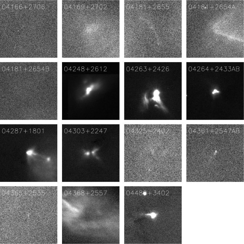
Figure 18: Keck/LRIS images of the Class I source sample defined by Kenyon et al. (1993a). Each panel shows a $30^{\prime\prime}\times 30^{\prime\prime}$ area. The LRIS images of the five sources analyzed in this paper are given in Figure 2, and those sources we did not analyze are shown here. Some of these objects are not detected in our observations, which may indicate different source luminosities or circumstellar dust geometries.

As discussed in §2.1, we obtained 0.9 $\mu$m images using Keck/LRIS of the entire sample studied by Kenyon et al. (1993a). The details of these observations are described in §2.3. Although the analysis presented above concentrated on only those sources that satisfied our selection criteria (§2.1), we display the LRIS images for the larger sample in Figure 18 for completeness.

Several of these objects are detected strongly at 0.9 $\mu$m: IRAS 04181+2654A, IRAS 04248+2612, IRAS 04263+2436, IRAS 04264+2433AB, IRAS 04287+1802, IRAS 04303+2247, IRAS 04361+2547AB, IRAS 04368+2557, and IRAS 04489+3402. Four other sources exhibit faint smudges that may correspond to actual emission: IRAS 04169+2702, IRAS 04181+2655, IRAS 04325+2402, and IRAS 04365+2635. The remaining sources were not detected, with a limiting $I$-band magnitude of $\sim 24$. Photometry for these objects, measured within a $6\hbox to0.0pt{.\hss}^{\prime\prime}3$ diameter aperture, is listed in White & Hillenbrand (2004).

Because these images are not very deep ($\leq 300$s), we can not comment on whether the pattern of detections and non-detections corresponds to variations in the underlying protostellar luminosities, different inclinations, or other factors. However, it is clear from Figure 18 that there are several sources exhibiting bright scattered light structures; these sources are ideal candidates for future work.

Figure 3: SEDs, scattered light images, and millimeter continuum images for a rotating, collapsing envelope with a range of mass accretion rates, spanning $10^{-6}$ to $10^{-5}$ M_⊙ yr^-1 ($\dot{M}$ increases from the bottom to top panels). This model assumes $R_{\rm c}=30$ AU, $R_{\rm out}=1000$ AU, and $i=45^{\circ}$. The $I$-band images were generated by convolving our model images with a $1^{\prime\prime}$ FWHM Gaussian, to simulate the seeing of our LRIS observations. Similarly, we convolved the 1 mm images with the actual beam that was used to observe IRAS 04016+2610. For both 0.9 $\mu$m and 1 mm images, the contour intervals are 20% of the peak flux, beginning at 20%. The noisy appearance of some of the model images in this and subsequent figures is due to the finite number of photons used in our Monte Carlo radiative transfer modeling, and does not reflect underlying substructure. As $\dot{M}$ increases, the strength of near-IR scattered emission decreases, although the shape of the emission broadens (note that for $\dot{M}=10^{-5}$ M_⊙ yr^-1, the scattered emission is undetected in our models). Higher mass accretion rates also produce larger mid-IR absorptions. While the appearance of millimeter images is relatively unaffected by changes in $\dot{M}$, the long-wavelength flux is enhanced for higher accretion rates.

Figure 4: SEDs, scattered light images, and millimeter continuum images for a rotating, collapsing envelope with a range of centrifugal radii, spanning 30 to 500 AU ($R_{\rm c}$ increases from the bottom to top panels). This model assumes $\dot{M}=10^{-6}$ M_⊙ yr^-1, $R_{\rm out}=1000$ AU, and $i=45^{\circ}$. Larger values of $R_{\rm c}$ lead to less spherically symmetric dust distributions, leading to increased absorption in the midplane, but less absorption out of the midplane. Thus, for large $R_{\rm c}$, the central star becomes visible directly. The centrifugal radius also represents a region of enhanced density, and thus larger $R_{\rm c}$ lead to significantly larger millimeter emission regions. In fact for $R_{\rm c}=500$ AU, the millimeter emission is almost completely over-resolved in our OVRO observations.

Figure 5: SEDs, scattered light images, and millimeter continuum images for a rotating, collapsing envelope with a range of outer radii, spanning 500 to 2000 AU ($R_{\rm out}$ increases from the bottom to top panels). This model assumes $\dot{M}=3\times 10^{-6}$ M_⊙ yr^-1, $R_{\rm c}=30$ AU, and $i=45^{\circ}$. As $R_{\rm out}$ increases, the amount of material in the envelope is increased (for a fixed $\dot{M}$), increasing the optical depth and leading to slightly higher absorption at near-to-mid-IR wavelengths. Not surprisingly, the images at both 0.9 $\mu$m and 1 mm become larger as $R_{\rm out}$ is increased. For the 1 mm images, the increased extended emission is manifested primarily by stronger sidelobe features, which are artifacts of the limited sampling in our interferometric observations (the 1 mm images have been convolved with the OVRO beam obtained for IRAS 04016+2610).

Figure 6: SEDs, scattered light images, and millimeter continuum images for a flared disk model at a range of viewing angles ($i$ increases from the bottom to top panels). More edge-on models exhibit deeper absorption at mid-IR wavelengths, and higher extinction of the central star. For small inclinations ($i\lesssim 30^{\circ}$), the central star is visible, and dominates the $I$-band emission. For moderate inclinations, an asymmetric scattered light structure is observed, while for nearly edge-on orientations, a symmetric, double-lobed structure is observed. The millimeter emission for this model is unresolved by our observations, and the model images are thus insensitive to inclination.

Figure 7: SEDs, scattered light images, and millimeter continuum images for a flared disk model with a range of disk masses ($M_{\rm disk}$ increases from the bottom to top panels). For this model, $R_{\rm out}=1000$ AU, $h_{0}=15$ AU, and $i=60^{\circ}$. Higher disk mass increases the optical depth of the model, leading to higher absorption at short wavelengths and enhanced emission at long wavelengths. In addition, if there is sufficient dust mass, the central star is obscured, and scattered light is visible at short wavelengths. The flux in millimeter continuum images is increased for higher disk mass, and the emission becomes slightly more extended.

Figure 8: SEDs, scattered light images, and millimeter continuum images for a flared disk model with a range of disk scale heights ($h_{0}$ increases from the bottom to top panels). This model assumes $M_{\rm disk}=5\times 10^{-2}$ M_⊙, $R_{\rm out}=1000$ AU, and $i=60^{\circ}$. Larger values of $h_{0}$ produce similar effects on the short-wavelength SED and scattered light images as larger values of $M_{\rm disk}$ (Figure 7); higher absorption, and increased visibility of scattered light. However, the effects on the longer-wavelength emission differ; higher values of $h_{0}$ increase the far-IR flux, but have little effect on millimeter fluxes and lead to slightly more compact morphologies at millimeter wavelengths (corresponding to weaker sidelobe emission features).

Figure 9: SEDs, scattered light images, and millimeter continuum images for a flared disk model with a range of outer radii ($R_{\rm out}$ increases from the bottom to top panels). This model assumes $M_{\rm disk}=5\times 10^{-2}$ M_⊙, $h_{0}=15$ AU, and $i=60^{\circ}$. Since we have fixed the disk mass, different values of $R_{\rm out}$ do not significantly affect the opacity of the model. However, a larger outer radius produces a larger surface area of cool dust, which leads to a slight enhancement of the long-wavelength flux. Moreover, larger $R_{\rm out}$ will produce larger images in both scattered light and millimeter emission (the short-wavelength images shown here are dominated by light from the central protostar, and thus no scattered emission is visible).

Figure 10: SEDs, scattered light images, and millimeter continuum images for a flared disk model at a range of viewing angles ($i$ increases from the bottom to top panels). This model assumes $M_{\rm disk}=5\times 10^{-2}$ M_⊙, $h_{0}=15$ AU, and $R_{\rm out}=1000$ AU. The effects of inclination on disk models are similar to those shown for envelope models in Figure 6. More edge-on models exhibit deeper absorption at mid-IR wavelengths, and higher extinction of the central star. For moderate inclinations ($i\lesssim 55^{\circ}$), the central star is visible, and dominates the $I$-band emission. For large inclinations, an asymmetric scattered light structure is observed, while for nearly edge-on orientations, a symmetric, double-lobed structure is observed. The millimeter emission becomes more extended in appearance as inclination increases, although this is a minor effect.

Figure 11: SEDs for envelope+disk models for a range of disk masses ($M_{\rm disk}$ increases from the bottom to top panels). The inclination of the models has been fixed at 45^∘. The envelope component of the model has the following properties: $\dot{M}=3\times 10^{-6}$ M_⊙ yr^-1, $M_{\ast}=0.5$ M_⊙, $R_{\rm c}=100$ AU, and $R_{\rm out}=1000$ AU. The various models illustrate the effect of adding progressively more massive (plotted bottom to top) disks to the model: $M_{\rm disk}=10^{-3}$, $10^{-2}$, and $1.0$ M_⊙. The main effect of the disk is on the SED long-ward of 100 $\mu$m, where the dense, cool dust in the disk component adds substantial flux. The 0.9 $\mu$m and 1 mm images are also affected slightly, becoming more centrally concentrated for larger disk masses.

Figure 12: SED data (Table A), 10 $\mu$m spectrum (Kessler-Silacci et al. 2005), 0.9 $\mu$m scattered light image, and 1.3 mm continuum image for IRAS 04016+2610, along with best-fit models for different assumed circumstellar geometries (Table 2). The observed images have been rotated on the sky by $-10^{\circ}$ (east of north) so that they have the same position angle definition as the models. Images have contour levels of 10% of the peak flux, beginning at 10% ($\sim 6\sigma$) for the 0.9 $\mu$m images and 30% ($\sim 2.5\sigma$) for the 1 mm images. While pure disk models do not provide an adequate match to the data, extincted disks, pure envelopes, and disk+envelopes match reasonably well. The disk+envelope, which provides the smallest residuals between model and data, is preferred.

Figure 13: SED data (Table A), 10 $\mu$m spectrum (Kessler-Silacci et al. 2005), 0.9 $\mu$m scattered light image, and 1.3 mm continuum image for IRAS 04108+2803B, along with best-fit models for different assumed circumstellar geometries (Table 2). The observed images have been rotated on the sky by $-90^{\circ}$ (east of north) so that they have the same position angle definition as the models. Images have contour levels of 10% of the peak flux, beginning at 30% ($\sim 2.5\sigma$) for the 0.9 $\mu$m images and 30% ($\sim 3\sigma$) for the 1 mm images. Disk+envelope and disk+extinction models provide the best match to the data for this source.

Figure 14: SED data (Table A), 10 $\mu$m spectrum (Kessler-Silacci et al. 2005), 0.9 $\mu$m scattered light image, and 1.3 mm continuum image for IRAS 04239+2436, along with best-fit models for different assumed circumstellar geometries (Table 2). The observed images have been rotated on the sky by $-120^{\circ}$ (east of north) so that they have the same position angle definition as the models. Images have contour levels of 10% of the peak flux, beginning at 20% ($\sim 2.5\sigma$) for the 0.9 $\mu$m images and 30% ($\sim 5\sigma$) for the 1 mm images. For this object, the best-fit to the complete data set is obtained for disk+extinction and disk+envelope models, although the SED and 10 $\mu$m spectra are fitted best by the disk+envelope model.

Figure 15: SED data (Table A), 10 $\mu$m spectrum (Kessler-Silacci et al. 2005), 0.9 $\mu$m scattered light image, and 1.3 mm continuum image for IRAS 04295+2251, along with best-fit models for different assumed circumstellar geometries (Table 2). The observed images have been rotated on the sky by $155^{\circ}$ (east of north) so that they have the same position angle definition as the models. Images have contour levels of 10% of the peak flux, beginning at 10% ($\sim 13\sigma$) for the 0.9 $\mu$m images and 30% ($\sim 5\sigma$) for the 1 mm images. Disk+envelope and disk+extinction models provide a good match to the data for this source. Note that the modeled 1 mm images are typically smaller than the observations in this case, since small values of $R_{\rm c}$ are preferred by the SED and $I$-band data, forcing the best-fit model to a smaller centrifugal radius, and thus a smaller 1 mm image (see Figure 4).

Figure 16: SED data (Table A), 10 $\mu$m spectrum (Kessler-Silacci et al. 2005), 0.9 $\mu$m scattered light image, and 1.3 mm continuum image for IRAS 04381+2540, along with best-fit models for different assumed circumstellar geometries (Table 2). The observed images have been rotated on the sky by $180^{\circ}$ (east of north) so that they have the same position angle definition as the models. Images have contour levels of 10% of the peak flux, beginning at 30% ($\sim 2\sigma$) for the 0.9 $\mu$m images and 30% ($\sim 2.5\sigma$) for the 1 mm images. While pure disk models and pure envelope models do not provide an adequate match to the data, extincted disks and disk+envelopes do. The disk+envelope and disk+extinction models provide the smallest residuals between models and data (Table 2).

Figure 17: Azimuthally-averaged radial profile of millimeter emission of best-fit models for IRAS 04016+2610 (Table 2). The pure envelope model (solid line) produces most of its millimeter emission near the centrifugal radius, 100 AU in this case. The pure disk model (dotted line) is more centrally-peaked, producing the majority of the millimeter emission at small radii. The disk+envelope model resembles the pure disk at small radii and the pure envelope at large radii.

Table 1: Spectral energy distributions for our sample

$\lambda$ ($\mu$m)	Source Fluxes, $F_{\nu}$ (Jy)					referencea
	04016+2610	04108+2803	04239+2436	04295+2251	04381+2540
0.55	2.42e-05					Kenyon et al. (1993a)
0.63	6.17e-05					Kenyon et al. (1993a)
0.79	0.0001					Kenyon et al. (1993a)
0.89	0.0001	3.23e-06	3.89e-05	2.23e-05	8.13e-06	This work
1.10	0.0003					Padgett et al. (1999)
1.22	0.0055	0.0004	0.0010	0.0055	0.0005	Kenyon et al. (1993a)
1.22				0.0038		Whitney et al. (1997)
1.60	0.0095					Padgett et al. (1999)
1.63	0.0217	0.0050	0.0075	0.0360	0.0018	Kenyon et al. (1993a)
1.63	0.0233	0.0242	0.0076	0.0229	0.0029	Park & Kenyon (2002)
1.63	0.0263	0.0043	0.0066	0.0220		Whitney et al. (1997)
1.87	0.0214					Padgett et al. (1999)
2.05	0.0416					Padgett et al. (1999)
2.19	0.1160	0.0226	0.0421	0.0943	0.0101	Kenyon et al. (1993a)
2.19	0.1045	0.0420	0.0464	0.0690	0.0147	Park & Kenyon (2002)
2.19	0.1055	0.0148	0.0439	0.0671	0.0149	Whitney et al. (1997)
3.45	0.4593	0.0492	0.2302	0.1667	0.0470	Kenyon et al. (1993a)
4.75	2.0465	0.1702				Kenyon et al. (1993a)
7.80	2.8	0.31				Myers et al. (1987)
8.69	2.10	0.50				Myers et al. (1987)
9.50	1.70	0.49				Myers et al. (1987)
10.3	2.50	0.57				Myers et al. (1987)
10.6	2.5682	0.6020		0.5883	0.2087	Kenyon et al. (1993a)
10.7	2.97	0.76	1.71	0.72	0.23	Kessler-Silacci et al. (2005)
11.6	3.40	0.44				Myers et al. (1987)
12.0	3.8327	0.7647	1.7120	0.6215	0.4106	Kenyon et al. (1993a)
12.5	4.90	1.30				Myers et al. (1987)
17.9	4.57			1.07		This work
21.0	10.6303	2.6094	4.4314		0.1979	Kenyon et al. (1993a)
25.0	16.3030	3.6498	6.9545	1.8718	2.7686	Kenyon et al. (1993a)
60.0	48.1371	7.6292	15.2222	3.4872	10.5312	Kenyon et al. (1993a)
100	62.2772	10.8225	17.1525	8.2097	14.9392	Kenyon et al. (1993a)
100	55.5046					Kenyon et al. (1993a)
160	46.6067					Kenyon et al. (1993a)
350	4.7686					Kenyon et al. (1993a)
450	3.2926	1.8094				Kenyon et al. (1993a)
450	2.8199				1.2000	Hogerheijde & Sandell (2000)
450	4.23	1.13	2.1400	2.6600	2.8199	Young et al. (2003)
800	0.582	0.085	0.3330	0.2410	0.2890	Moriarty-Schieven et al. (1994)
800	0.3143	0.8859	2.3303			Kenyon et al. (1993a)
850	0.5899	0.1700	0.4199	0.4199	0.5600	Young et al. (2003)
850	0.43				0.24	Hogerheijde & Sandell (2000)
1100	0.180	$<$0.100	0.114	0.094	0.116	Moriarty-Schieven et al. (1994)
1100	0.5317	0.0882	0.0768			Kenyon et al. (1993a)
1300	0.150	0.039	0.170	0.115	0.300	Motte & André (2001)
1300	0.0658	0.0271	0.0329	0.0484	0.0135	This work
2700	$<$0.0068				$<$0.0075	Hogerheijde et al. (1997)
3000	$<$0.0096	$<$0.0210	$<$0.0120	$<$0.0210		Ohashi et al. (1996)
3000		0.0058	0.0120	0.0087		This work
3369	$<$0.0043				$<$0.0050	Hogerheijde et al. (1997)
3440	$<$0.0180		$<$0.0240			Saito et al. (2001)
20000	0.0005					Lucas et al. (2000)
35000	0.0003		0.0001			Lucas et al. (2000)
60000	$<$0.0002					Lucas et al. (2000)

References. — ^a–Kenyon et al. (1993a) compiled SEDs from new data and the literature, and this work contains references for much of this photometry.

Note. — Different observations were conducted with different angular resolutions, which explains some of the photometric variations. In addition, all of the sources in our sample except IRAS 04295+2251 are known to be variable at short wavelengths (e.g., Park & Kenyon 2002).

Table 2: Best-fit Models

Source	$\chi_{\rm r,tot}^{2}$	$\chi^{2}_{\rm r,SED}$	$\chi^{2}_{\rm r,0.9\mu m}$	$\chi^{2}_{\rm r,1mm}$	$\dot{M}$	$R_{\rm c}$	$M_{\rm env}$	$M_{\rm disk}$	$h_{0}$	$R_{\rm out}$	$i$	$L_{\rm central}$
					(M⊙ yr-1)	(AU)	(M⊙)	(M⊙)	(AU)	(AU)	(∘)	(L⊙)
Rotating Infalling Envelope Models
IRAS 04016+2610	4.39	1.57	1.40	1.41	$8\times 10^{-6}$	100	$0.07$	$...$	…	2000	36	3.8
IRAS 04108+2803B	5.25	2.90	1.08	1.26	$6\times 10^{-6}$	30	$0.05$	$...$	…	2000	26	0.7
IRAS 04239+2436	6.89	3.93	1.17	1.77	$8\times 10^{-6}$	100	$0.07$	$...$	…	2000	42	2.3
IRAS 04295+2251	13.07	10.05	1.21	1.79	$9\times 10^{-6}$	100	$0.01$	$...$	…	500	34	1.1
IRAS 04381+2540	4.25	1.93	1.01	1.30	$1\times 10^{-5}$	100	$0.10$	$...$	…	2000	30	0.6
Flared Disk Models
IRAS 04016+2610	14.30	9.68	3.35	1.24	$...$	…	$...$	$0.10$	25	2000	52	2.8
IRAS 04108+2803B	12.81	10.30	1.28	1.21	$...$	…	$...$	$0.10$	25	500	52	2.3
IRAS 04239+2436	11.21	8.18	1.73	1.30	$...$	…	$...$	$1.00$	25	500	45	1.0
IRAS 04295+2251	13.98	10.60	2.26	1.11	$...$	…	$...$	$1.00$	15	1000	55	0.9
IRAS 04381+2540	9.70	7.56	1.03	1.10	$...$	…	$...$	$0.70$	15	2000	56	0.5
Disk+Envelope Models
IRAS 04016+2610	4.12	1.35	1.51	1.25	$6\times 10^{-6}$	100	$0.05$	$0.01$	15	2000	37	4.7
IRAS 04108+2803B	3.68	1.40	1.04	1.22	$5\times 10^{-6}$	30	$5\times 10^{-3}$	$0.50$	15	500	24	0.4
IRAS 04239+2436	4.73	1.67	1.72	1.33	$3\times 10^{-6}$	30	$0.01$	$0.50$	15	1000	34	1.5
IRAS 04295+2251	5.83	2.75	1.93	1.13	$5\times 10^{-6}$	30	$5\times 10^{-3}$	$1.00$	15	500	22	0.6
IRAS 04381+2540	3.47	1.34	1.04	1.08	$9\times 10^{-6}$	30	$0.01$	$1.00$	15	1000	34	0.6
Disk+Extinction Models
IRAS 04016+2610	6.28	1.82	3.20	1.25	$...$	…	AV=10	$0.20$	25	2000	49	5.3
IRAS 04108+2803B	3.34	1.07	1.05	1.21	$...$	…	AV=25	$0.60$	25	500	17	0.6
IRAS 04239+2436	5.01	2.44	1.21	1.35	$...$	…	AV=20	$0.20$	20	2000	50	5.4
IRAS 04295+2251	4.42	1.08	2.24	1.09	$...$	…	AV=20	$1.00$	15	500	49	1.2
IRAS 04381+2540	3.27	1.12	1.06	1.07	$...$	…	AV=20	$0.70$	15	500	56	1.0

Note. — Best-fit models for different density distributions considered in §3. $\chi^{2}_{\rm r,tot}$ is the sum of the reduced chi-squared residuals between the data and model for the SED, 0.9 $\mu$m, and 1 mm images. The individual reduced chi squared values for each dataset are denoted by $\chi^{2}_{\rm r,SED}$, $\chi^{2}_{\rm r,0.9\mu m}$, and $\chi^{2}_{\rm r,1mm}$. In the case of the disk+extinction models, entries in the $M_{\rm env}$ column correspond to foreground extinction. Although the disk masses listed in this Table are the results of our model-fitting, we believe that these are likely over-estimated (§5.2).

Table 3: Comparison of compact and large-scale millimeter emission

Source	$R_{\rm data}$	$R_{\rm disk}$	$R_{\rm env}$	$R_{\rm disk+env}$
IRAS 04016+2610	0.43	0.17	0.06	0.15
IRAS 04108+2803B	0.70	0.60	0.08	0.57
IRAS 04239+2436	0.19	0.53	0.06	0.29
IRAS 04295+2251	0.42	0.28	0.26	0.35
IRAS 04381+2540	0.05	0.12	0.05	0.32

References. — In this table, $R_{\rm data}$ is the ratio of emission observed in our compact OVRO beam to the emission observed in the larger-beam survey of Motte & André (2001). $R_{\rm disk}$, $R_{\rm env}$, and $R_{\rm disk+env}$ are the ratios one would measure for pure disk, pure envelope, and disk+envelope models. For disk+extinction models (§3.4), the distribution of large-scale material is unconstrained, and thus we do not calculate expected ratios for these models.

References

- Adams et al. (1987) Adams, F. C., Lada, C. J., & Shu, F. H. 1987, ApJ, 312, 788
- André & Montmerle (1994) André, P. & Montmerle, T. 1994, ApJ, 420, 837
- André et al. (1993) André, P., Ward-Thompson, D., & Barsony, M. 1993, ApJ, 406, 122
- Bèland et al. (1988) Bèland, S., Boulade, O., & Davidge, T. 1988, Bulletin d’information du telescope Canada-France-Hawaii, 19, 16
- Beichman et al. (1986) Beichman, C. A., Myers, P. C., Emerson, J. P., Harris, S., Mathieu, R., Benson, P. J., & Jennings, R. E. 1986, ApJ, 307, 337
- Bell & Lin (1994) Bell, K. R. & Lin, D. N. C. 1994, ApJ, 427, 987
- Benson & Myers (1989) Benson, P. J. & Myers, P. C. 1989, ApJS, 71, 89
- Brown & Chandler (1999) Brown, D. W. & Chandler, C. J. 1999, MNRAS, 303, 855
- Butner et al. (1991) Butner, H. M., Evans, N. J., Lester, D. F., Levreault, R. M., & Strom, S. E. 1991, ApJ, 376, 636
- Calvet & Gullbring (1998) Calvet, N. & Gullbring, E. 1998, ApJ, 509, 802
- Cassen & Moosman (1981) Cassen, P. & Moosman, A. 1981, Icarus, 48, 353
- Chandler & Richer (2000) Chandler, C. J. & Richer, J. S. 2000, ApJ, 530, 851
- Chandler et al. (1996) Chandler, C. J., Terebey, S., Barsony, M., Moore, T. J. T., & Gautier, T. N. 1996, ApJ, 471, 308
- Chiang & Goldreich (1997) Chiang, E. I. & Goldreich, P. 1997, ApJ, 490, 368
- Chiang & Goldreich (1999) —. 1999, ApJ, 519, 279
- D’Alessio et al. (2001) D’Alessio, P., Calvet, N., & Hartmann, L. 2001, ApJ, 553, 321
- D’Alessio et al. (1999) D’Alessio, P., Calvet, N., Hartmann, L., Lizano, S., & Cantó, J. 1999, ApJ, 527, 893
- Draine & Lee (1984) Draine, B. T. & Lee, H. M. 1984, ApJ, 285, 89
- Draine & Malhotra (1993) Draine, B. T. & Malhotra, S. 1993, ApJ, 414, 632
- Duchêne et al. (2004) Duchêne, G., Bouvier, J., Bontemps, S., André, P., & Motte, F. 2004, A&A, 427, 651
- Dullemond et al. (2001) Dullemond, C. P., Dominik, C., & Natta, A. 2001, ApJ, 560, 957
- Eisner et al. (2003) Eisner, J. A., Lane, B. F., Akeson, R. L., Hillenbrand, L., & Sargent, A. 2003, ApJ, 588, 360
- Eisner et al. (2004) Eisner, J. A., Lane, B. F., Hillenbrand, L., Akeson, R., & Sargent, A. 2004, ApJ, 613, 1049
- Galli & Shu (1993a) Galli, D. & Shu, F. H. 1993a, ApJ, 417, 220
- Galli & Shu (1993b) —. 1993b, ApJ, 417, 243
- Goldreich & Ward (1973) Goldreich, P. & Ward, W. R. 1973, ApJ, 183, 1051
- Gomez et al. (1997) Gomez, M., Whitney, B. A., & Kenyon, S. J. 1997, AJ, 114, 1138
- Grady et al. (1999) Grady, C. A., Woodgate, B., Bruhweiler, F. C., Boggess, A., Plait, P., Lindler, D. J., Clampin, M., & Kalas, P. 1999, ApJ, 523, L151
- Gullbring et al. (2000) Gullbring, E., Calvet, N., Muzerolle, J., & Hartmann, L. 2000, ApJ, 544, 927
- Gullbring et al. (1998) Gullbring, E., Hartmann, L., Briceno, C., & Calvet, N. 1998, ApJ, 492, 323
- Hartmann (1998) Hartmann, L. 1998, Accretion processes in star formation (Accretion processes in star formation / Lee Hartmann. Cambridge, UK ; New York : Cambridge University Press, 1998. (Cambridge astrophysics series ; 32) ISBN 0521435072.)
- Hartmann & Kenyon (1996) Hartmann, L. & Kenyon, S. J. 1996, ARA&A, 34, 207
- Hogerheijde (2001) Hogerheijde, M. R. 2001, ApJ, 553, 618
- Hogerheijde & Sandell (2000) Hogerheijde, M. R. & Sandell, G. 2000, ApJ, 534, 880
- Hogerheijde et al. (1997) Hogerheijde, M. R., van Dishoeck, E. F., Blake, G. A., & van Langevelde, H. J. 1997, ApJ, 489, 293
- Hogerheijde et al. (1998) —. 1998, ApJ, 502, 315
- Ishii et al. (2004) Ishii, M., Tamura, M., & Itoh, Y. 2004, ApJ, 612, 956
- Jones & Puetter (1993) Jones, B. & Puetter, R. C. 1993, in Proc. SPIE Vol. 1946, p. 610-621, Infrared Detectors and Instrumentation, Albert M. Fowler; Ed., 610–621
- Keene & Masson (1990) Keene, J. & Masson, C. R. 1990, ApJ, 355, 635
- Kenyon et al. (1993a) Kenyon, S. J., Calvet, N., & Hartmann, L. 1993a, ApJ, 414, 676
- Kenyon & Hartmann (1987) Kenyon, S. J. & Hartmann, L. 1987, ApJ, 323, 714
- Kenyon & Hartmann (1995) —. 1995, ApJS, 101, 117
- Kenyon et al. (1990) Kenyon, S. J., Hartmann, L. W., Strom, K. M., & Strom, S. E. 1990, AJ, 99, 869
- Kenyon et al. (1993b) Kenyon, S. J., Whitney, B. A., Gomez, M., & Hartmann, L. 1993b, ApJ, 414, 773
- Kessler-Silacci et al. (2005) Kessler-Silacci, J. E., Hillenbrand, L. A., Blake, G. A., & Meyer, M. R. 2005, ApJ, 622, 404
- Koerner & Sargent (1995) Koerner, D. W. & Sargent, A. I. 1995, AJ, 109, 2138
- Lada (1987) Lada, C. J. 1987, in IAU Symp. 115, Star Forming Regions, ed. M. Peimbert & J. Jugaku (Dordrecht: Reidel), 1
- Lada & Wilking (1984) Lada, C. J. & Wilking, B. A. 1984, ApJ, 287, 610
- Ladd et al. (1995) Ladd, E. F., Fuller, G. A., Padman, R., Myers, P. C., & Adams, F. C. 1995, ApJ, 439, 771
- Landolt (1992) Landolt, A. U. 1992, AJ, 104, 340
- Larson (1969) Larson, R. B. 1969, MNRAS, 145, 271
- Laughlin & Bodenheimer (1994) Laughlin, G. & Bodenheimer, P. 1994, ApJ, 436, 335
- Lay et al. (1994) Lay, O. P., Carlstrom, J. E., Hills, R. E., & Phillips, T. G. 1994, ApJ, 434, L75
- Leinert et al. (2004) Leinert, C., van Boekel, R., Waters, L. B. F. M., Chesneau, O., Malbet, F., Köhler, R., Jaffe, W., Ratzka, T., Dutrey, A., Preibisch, T., Graser, U., Bakker, E., Chagnon, G., Cotton, W. D., Dominik, C., Dullemond, C. P., Glazenborg-Kluttig, A. W., Glindemann, A., Henning, T., Hofmann, K.-H., de Jong, J., Lenzen, R., Ligori, S., Lopez, B., Meisner, J., Morel, S., Paresce, F., Pel, J.-W., Percheron, I., Perrin, G., Przygodda, F., Richichi, A., Schöller, M., Schuller, P., Stecklum, B., van den Ancker, M. E., von der Lühe, O., & Weigelt, G. 2004, A&A, 423, 537
- Lucas et al. (2000) Lucas, P. W., Blundell, K. M., & Roche, P. F. 2000, MNRAS, 318, 526
- Lucas & Roche (1998) Lucas, P. W. & Roche, P. F. 1998, MNRAS, 299, 699
- Mathis et al. (1977) Mathis, J. S., Rumpl, W., & Nordsieck, K. H. 1977, ApJ, 217, 425
- McCaughrean & O’Dell (1996) McCaughrean, M. J. & O’Dell, C. R. 1996, AJ, 111, 1977
- Monnier et al. (2004) Monnier, J. D., Tuthill, P. G., Ireland, M. J., Cohen, R., & Tannirkulam, A. 2004, American Astronomical Society Meeting Abstracts, 205,
- Moriarty-Schieven et al. (1994) Moriarty-Schieven, G. H., Wannier, P. G., Keene, J., & Tamura, M. 1994, ApJ, 436, 800
- Moriarty-Schieven et al. (1992) Moriarty-Schieven, G. H., Wannier, P. G., Tamura, M., & Keene, J. 1992, ApJ, 400, 260
- Motte & André (2001) Motte, F. & André, P. 2001, A&A, 365, 440
- Myers et al. (1987) Myers, P. C., Fuller, G. A., Mathieu, R. D., Beichman, C. A., Benson, P. J., Schild, R. E., & Emerson, J. P. 1987, ApJ, 319, 340
- Myers et al. (1988) Myers, P. C., Heyer, M., Snell, R. L., & Goldsmith, P. F. 1988, ApJ, 324, 907
- Nakazato et al. (2003) Nakazato, T., Nakamoto, T., & Umemura, M. 2003, ApJ, 583, 322
- Ohashi et al. (1996) Ohashi, N., Hayashi, M., Kawabe, R., & Ishiguro, M. 1996, ApJ, 466, 317
- Oke et al. (1995) Oke, J. B., Cohen, J. G., Carr, M., Cromer, J., Dingizian, A., Harris, F. H., Labrecque, S., Lucinio, R., Schaal, W., Epps, H., & Miller, J. 1995, PASP, 107, 375
- Osorio et al. (2003) Osorio, M., D’Alessio, P., Muzerolle, J., Calvet, N., & Hartmann, L. 2003, ApJ, 586, 1148
- Padgett et al. (1999) Padgett, D. L., Brandner, W., Stapelfeldt, K. R., Strom, S. E., Terebey, S., & Koerner, D. 1999, AJ, 117, 1490
- Park & Kenyon (2002) Park, S. & Kenyon, S. J. 2002, AJ, 123, 3370
- Pascucci et al. (2004) Pascucci, I., Wolf, S., Steinacker, J., Dullemond, C. P., Henning, T., Niccolini, G., Woitke, P., & Lopez, B. 2004, A&A, 417, 793
- Rodriguez et al. (1998) Rodriguez, L. F., D’Alessio, P., Wilner, D. J., Ho, P. T. P., Torrelles, J. M., Curiel, S., Gomez, Y., Lizano, S., Pedlar, A., Canto, J., & Raga, A. C. 1998, Nature, 395, 355
- Saito et al. (2001) Saito, M., Kawabe, R., Kitamura, Y., & Sunada, K. 2001, ApJ, 547, 840
- Sault et al. (1995) Sault, R. J., Teuben, P. J., & Wright, M. C. H. 1995, in ASP Conf. Ser. 77: Astronomical Data Analysis Software and Systems IV, 433–+
- Scoville et al. (1993) Scoville, N. Z., Carlstrom, J. E., Chandler, C. J., Phillips, J. A., Scott, S. L., Tilanus, R. P. J., & Wang, Z. 1993, PASP, 105, 1482
- Semenov et al. (2004) Semenov, D., Pavlyuchenkov, Y., Schreyer, K., Henning, T., Dullemond, C., & Bacmann, A. 2004, ArXiv Astrophysics e-prints
- Shakura & Sunyaev (1973) Shakura, N. I. & Sunyaev, R. A. 1973, A&A, 24, 337
- Shu et al. (1993) Shu, F., Najita, J., Galli, D., Ostriker, E., & Lizano, S. 1993, in Protostars and Planets III, 3–45
- Shu (1977) Shu, F. H. 1977, ApJ, 214, 488
- Shu et al. (1987) Shu, F. H., Adams, F. C., & Lizano, S. 1987, ARA&A, 25, 23
- Strom et al. (1976) Strom, K. M., Strom, S. E., & Vrba, F. J. 1976, AJ, 81, 320
- Su et al. (2005) Su, K. Y. L., Rieke, G. H., Misselt, K. A., Stansberry, J. A., Moro-Martin, A., Stapelfeldt, K. R., Werner, M. W., Trilling, D. E., Bendo, G. J., Gordon, K. D., Hines, D. C., Wyatt, M. C., Holland, W. S., Marengo, M., Megeath, S. T., & Fazio, G. G. 2005, ArXiv Astrophysics e-prints
- Tamura et al. (1991) Tamura, M., Gatley, I., Waller, W., & Werner, M. W. 1991, ApJ, 374, L25
- Terebey et al. (1984) Terebey, S., Shu, F. H., & Cassen, P. 1984, ApJ, 286, 529
- Terebey et al. (1989) Terebey, S., Vogel, S. N., & Myers, P. C. 1989, ApJ, 340, 472
- Terquem & Bertout (1996) Terquem, C. & Bertout, C. 1996, MNRAS, 279, 415
- Ulrich (1976) Ulrich, R. K. 1976, ApJ, 210, 377
- Watson et al. (2004) Watson, D. M., Kemper, F., Calvet, N., Keller, L. D. Furlan, E., Hartmann, L., Forrest, W. J., Chen, C. H., Uchida, K. I., Green, J. D., Sargent, B., Sloan, G. C., Herter, T. L., Brandl, B. R., Houck, J. R., Najita, J., D’Alessio, P., Myers, P. C., Barry, D. J., Hall, P., & Morris, P. W. 2004, ApJS, 154, 391
- Weingartner & Draine (2001) Weingartner, J. C. & Draine, B. T. 2001, ApJ, 548, 296
- White et al. (2000) White, G. J., Liseau, R., Men’shchikov, A. B., Justtanont, K., Nisini, B., Benedettini, M., Caux, E., Ceccarelli, C., Correia, J. C., Giannini, T., Kaufman, M., Lorenzetti, D., Molinari, S., Saraceno, P., Smith, H. A., Spinoglio, L., & Tommasi, E. 2000, A&A, 364, 741
- White & Hillenbrand (2004) White, R. J. & Hillenbrand, L. A. 2004, ApJ, 616, 998
- Whitney & Hartmann (1992) Whitney, B. A. & Hartmann, L. 1992, ApJ, 395, 529
- Whitney et al. (1997) Whitney, B. A., Kenyon, S. J., & Gomez, M. 1997, ApJ, 485, 703
- Whitney et al. (2003a) Whitney, B. A., Wood, K., Bjorkman, J. E., & Cohen, M. 2003a, ApJ, 598, 1079
- Whitney et al. (2003b) Whitney, B. A., Wood, K., Bjorkman, J. E., & Wolff, M. J. 2003b, ApJ, 591, 1049
- Wolf (2003) Wolf, S. 2003, Computer Physics Communications, 150, 99
- Wolf & Henning (2000) Wolf, S. & Henning, T. 2000, Computer Physics Communications, 132, 166
- Wolf et al. (1999) Wolf, S., Henning, T., & Stecklum, B. 1999, A&A, 349, 839
- Wolf et al. (2003) Wolf, S., Padgett, D. L., & Stapelfeldt, K. R. 2003, ApJ, 588, 373
- Wood et al. (2002) Wood, K., Wolff, M. J., Bjorkman, J. E., & Whitney, B. 2002, ApJ, 564, 887
- Yorke et al. (1995) Yorke, H. W., Bodenheimer, P., & Laughlin, G. 1995, ApJ, 443, 199
- Young et al. (2003) Young, C. H., Shirley, Y. L., Evans, N. J., & Rawlings, J. M. C. 2003, ApJS, 145, 111