Nebular Spectra of SN 1998bw Revisited:
Detailed Study by One and Two Dimensional Models

Abstract

Refined one- and two-dimensional models for the nebular spectra of the hyper-energetic Type Ic supernova (SN) 1998bw, associated with the gamma-ray burst GRB980425, from 125 to 376 days after B-band maximum are presented. One dimensional, spherically symmetric spectrum synthesis calculations show that reproducing features in the observed spectra, i.e., the sharply peaked [OI] 6300Å doublet and MgI] 4570Å emission, and the broad [FeII] blend around 5200Å, requires the existence of a high-density O-rich core expanding at low velocities ($\mathrel{\hbox to0.0pt{\lower 4.0pt\hbox{\hskip 1.0pt$\sim$}\hss}\raise 1.0pt\hbox{$<$}}8,000$ km s^-1) and of Fe-rich material moving faster than the O-rich material. Synthetic spectra at late phases from aspherical (bipolar) explosion models are also computed with a two-dimensional spectrum synthesis code. The above features are naturally explained by the aspherical model if the explosion is viewed from a direction close to the axis of symmetry ($\sim 30^{\rm o}$), since the aspherical model yields a high-density O-rich region confined along the equatorial axis. By examining a large parameter space (in energy and mass), our best model gives following physical quantities: the kinetic energy $E_{51}\equiv E_{\rm K}/10^{51}$ ergs $\mathrel{\hbox to0.0pt{\lower 4.0pt\hbox{\hskip 1.0pt$\sim$}\hss}\raise 1.0pt\hbox{$>$}}8-12$ and the main-sequence mass of the progenitor star $M_{\rm ms}\mathrel{\hbox to0.0pt{\lower 4.0pt\hbox{\hskip 1.0pt$\sim$}\hss}\raise 1.0pt\hbox{$>$}}30-35M_{\odot}$. The temporal spectral evolution of SN 1998bw also indicates mixing among Fe-, O-, and C-rich regions, and highly clumpy structure.

1 INTRODUCTION

There has been accumulating evidence that a class of supernovae (SNe) is related to long-duration Gamma-Ray Bursts (GRBs; see Piran 1999 for a review) and possibly to their low energy analog, X-Ray Flashes (XRFs; Heise et al. 2001). The discovery of SN 1998bw in the error box of GRB 980425 (Galama et al. 1998) raised the issue, and now the association between GRBs and SNe is firmly confirmed by the emergence of supernova spectra in the optical afterglows of some GRBs, i.e., SN 2003dh/GRB 030329 (Hjorth et al. 2003; Kawabata et al. 2003; Matheson et al. 2003; Stanek et al. 2003), SN 2003lw/GRB 031203 (Malesani et al. 2004; Thomsen et al. 2004, Mazzali et al., in preparation), and SN 2002lt/GRB 021211 (Della Valle et al. 2003).

All these supernovae (except SN 2002lt) seem to belong to a special class (see e.g., Matheson 2004 for a review). Their spectra near maximum optical brightness are characterized by significant blending of very broad lines. A popular idea to explain this feature in the GRB-related supernovae is a hyper-energetic explosion ($E_{51}\equiv E_{\rm K}/10^{51}$ ergs $\mathrel{\hbox to0.0pt{\lower 4.0pt\hbox{\hskip 1.0pt$\sim$}\hss}\raise 1.0pt\hbox{$>$}}5-10$) of a very massive star ($M_{\rm ms}\mathrel{\hbox to0.0pt{\lower 4.0pt\hbox{\hskip 1.0pt$\sim$}\hss}\raise 1.0pt\hbox{$>$}}20-25M_{\odot}$). Such an energetic supernova is often called a ”hypernova” (Iwamoto et al. 1998; Nomoto et al. 2004), with a somewhat different use of the original terminology suggested by Paczynski (1998) to describe the entire GRB/afterglow phenomenon.

The nature of GRBs and hypernovae, and their mutual relation, are still the subject of debate. Asphericity seems to be the key to understand both GRBs and hypernovae. It is widely accepted that GRBs are produced by a relativistic jet viewed on or near its axis (Frail et al. 2001; Bloom, Frail, & Kulkarni 2003). Their physical link to hypernovae then suggests that hypernovae also should show signatures of asphericity, according to popular progenitor scenarios: a black-hole plus an accretion disk (Woosley 1993; MacFadyen & Woosley 1999; Brown et al. 2000), or a highly magnetized neutron star (Nakamura 1998; Wheeler et al. 2000).

The hypernova models for the GRB-related supernovae have been developed on the basis of modeling early phase observations up to $\sim$ 2 months after the explosion. For SN 1998bw, photometric and spectroscopic observations covering more than 1 year are available (Sollerman et al. 2000; Patat et al. 2001). Since SN 1998bw was the first supernova being identified as the counterpart of a GRB (GRB980425), and it has been extensively referred to as a prototypical hypernova, it is important to understand its nature.

Studying the late phase light curve and spectra has provided additional hints on the nature of SN 1998bw. While the early phase observations can be reproduced by a ”spherical” hypernova model (Iwamoto et al. 1998; Woosley, Eastman, & Schmidt 1999; Nakamura et al. 2001), the light curve after $\sim 2$ months declined less steeply than the spherical hypernova model prediction (McKenzie & Schaefer 1999). A similar problem exists for other hypernovae (e.g., Mazzali, Iwamoto, & Nomoto 2000; Yoshii et al. 2003) and some SNe IIb/Ib/Ic (e.g., Clocchiatti & Wheeler 1997). For hypernovae, Maeda et al. (2003a) attributed the failure of the spherical models to the possible existence of an inner low-velocity dense core, which may be formed as the consequence of an aspherical explosion (e.g., Maeda & Nomoto 2003b).

Late phase spectra provide an excellent tool to examine the geometry of the ejecta, as they can probe deeper than the early-phase spectra. The nebular spectra of SN 1998bw showed peculiar features which were not explained by a simple picture (Patat et al. 2001). First, the [OI] 6300Å & 6363Å doublet shows a sharply peaked emission profile. The profile is different from both the parabolic profile expected from a homogeneous spherical distribution of emitting material and the flat-topped boxy profile expected from material distributed in a shell. Sollerman et al. (2000) found that both the spherical hypernova model CO138 of Iwamoto et al. (1998) (CO138E30; the explosion with $E_{51}=30$ of a $13.8M_{\odot}$ CO star evolved from a zero-age main sequence star of $M_{\rm ms}\sim 40M_{\odot}$), and CO6C of Woosley et al. (1999) ($E_{51}=22$, a 6.55 $M_{\odot}$ CO star, and $M_{\rm ms}\sim 25M_{\odot}$) yielded too broad [OI] 6300Å emission. The feature near 5200Å, interpreted as a blend of [FeII] in Mazzali et al. (2001) and Maeda et al. (2002) also shows a peculiarity: it is broader than the [OI] 6300Å. Mazzali et al. (2001) showed that each line contributing to the [FeII] blend should be broader than the [OI] 6300Å, i.e., velocities of once-ionized iron ions should be higher than those of neutral oxygen along the line of sight. Subsequently, Maeda et al. (2002) computed the theoretical line profiles expected from bipolar aspherical models. They showed that the peculiarity of the [OI] 6300Å and [FeII] 5200Å emissions in SN 1998bw can be explained by the aspherical explosion models, if the axis of symmetry is roughly aligned with the line of sight.

Although these previous studies revealed the peculiarities and suggested possible solutions, there were still some limitations. As for one dimensional models, previous studies (Sollerman et al. 2000; Mazzali et al. 2001) did not model the full set of late-phase spectra at various epochs on the basis of a hydrodynamic model. Concerning two dimensional models, the analysis of Maeda et al. (2002) had the following limitations. (1) First, they applied a simplified time-independent computation for the line profiles. (2) They did not model the flux. A more detailed analysis based on nebular line emission physics is necessary to derive the nature, e.g., the explosion energy, of the explosion. (3) Also, it should be examined if their models, focusing on the [FeII] 5200Å and the [OI] 6300Å, are consistent with other emission lines, e.g., MgI] 4570Å and [CaII] 7300Å. (4) Their model grid (in energy and mass) was rather coarse. To constrain physical values such as the energy, models with various energies and masses should be examined comprehensively. (5) Finally, they only examined one nebular spectrum (+216 days after the maximum optical luminosity). It is important to examine if ”one” model can consistently reproduce the temporal evolution of spectra.

The purpose of this paper is to perform a more detailed analysis of the nebular spectra of SN 1998bw than previous works. In addition to one dimensional spectrum synthesis, we use a two dimensional nebular spectrum synthesis code, which includes two-dimensional $\gamma$-ray transfer and a computation of ionization/thermal structures for two-dimensional density and abundance distributions. First, the nebular spectra of SN 1998bw are examined by means of one dimensional spectrum synthesis in §2, to obtain conditions necessary to explain the spectra of SN 1998bw. The subsequent parts are devoted to the two dimensional models. In §3 we describe models and method, and present a comparison between the synthetic spectra and the observations. Summary and discussion are presented in §4.

2 ONE DIMENSIONAL MODELS

2.1 Method

We use a non-LTE code to compute nebular spectra. The code is an extension of the one-zone nebular code of Mazzali et al. (2001), allowing radially stratified density and abundance distributions as an input model. First, a Monte-Carlo Method (e.g., Cappellaro et al. 1997; Chugai 2000; Maeda et al. 2003a) is used to solve the transport of $\gamma$-rays released by the decay chain ⁵⁶Ni $\to$ ⁵⁶Co$\to$ ⁵⁶Fe. Positrons released by the same decay chain are assumed to be trapped in situ (Axelrod 1980). The light curve of SN 1998bw suggests that at a few hundred days $\gamma$-rays are still the dominant heating source (Nakamura et al. 2001; Maeda et al. 2003a), making the heating of the ejecta little sensitive to the detail of positron transport (e.g., Milne, The, & Leising 2001).

Next, ionization and NLTE thermal balance in each shell are solved on the basis of the prescription given by Ruiz-Lapuente & Lucy (1992). For the ionization source, we consider only impact ionizations by high-energy particles produced by the deposition of $\gamma$-rays (and $e^{+}$). The ionization balance is then solved by equating the impact ionization rate to the recombination rate for each ion. An assumption here is that photoionization is negligible. Although it is still a matter of debate (see e.g., Sollerman et al. 2004), it is argued that large multiple resonance scattering at high energies effectively reduces the UV radiation, therefore reduces the photoionizations (Kozma & Fransson 1998b; Kozma et al. 2005). Level populations are obtained by solving rate equations in steady state for each level along with the thermal balance (i.e., equating of the non-thermal heating rate and the line cooling rate). We consider mainly forbidden lines as a source of cooling (Ruiz-Lapuente & Lucy 1992), but strong allowed transitions, e.g., CaII IR, are also included. Under nebular conditions, radiative losses are entirely due to collisionally excited lines. We do not take radiation transfer effects into account, since the epochs examined in the present work are later than $100$ days so that radiation transfer effects are usually small at least at optical wavelengths (see §4.5.1 for more detail). Observationally, after day $100\sim 200$, neither the feature at 4570Å nor that at 6300Å evolved significantly (Patat et al. 2001), indicating that these features are totally dominated by forbidden lines and that radiation transfer effects are negligible. In particular, we do not include line scattering and fluorescence, an assumption that is usually made in nebular analysis (e.g., Kozma et al. 2005). Fluorescence may have effects in some lines, i.e., Ca II H, K and IR-triplet, and NaI (Kozma & Fransson 1998b), for which we do not present detailed modeling in the present work. Finally, a synthetic spectrum is obtained by integrating the emission from each shell.

Throughout the paper, synthetic spectra are compared with the spectra of SN 1998bw taken at 125, 200, 337, and 376 days after B maximum (Patat et al. 2001). The first spectrum ($+125^{\rm d}$) may not fully be nebular and hence can not be fully interpreted using the present computational code (see §4). Despite this, we include this spectrum in the comparison. The spectrum is at least partly nebular and therefore can still be used to reject any model producing a spectrum very different from it.

2.2 SN 1998bw: One Dimensional Approach

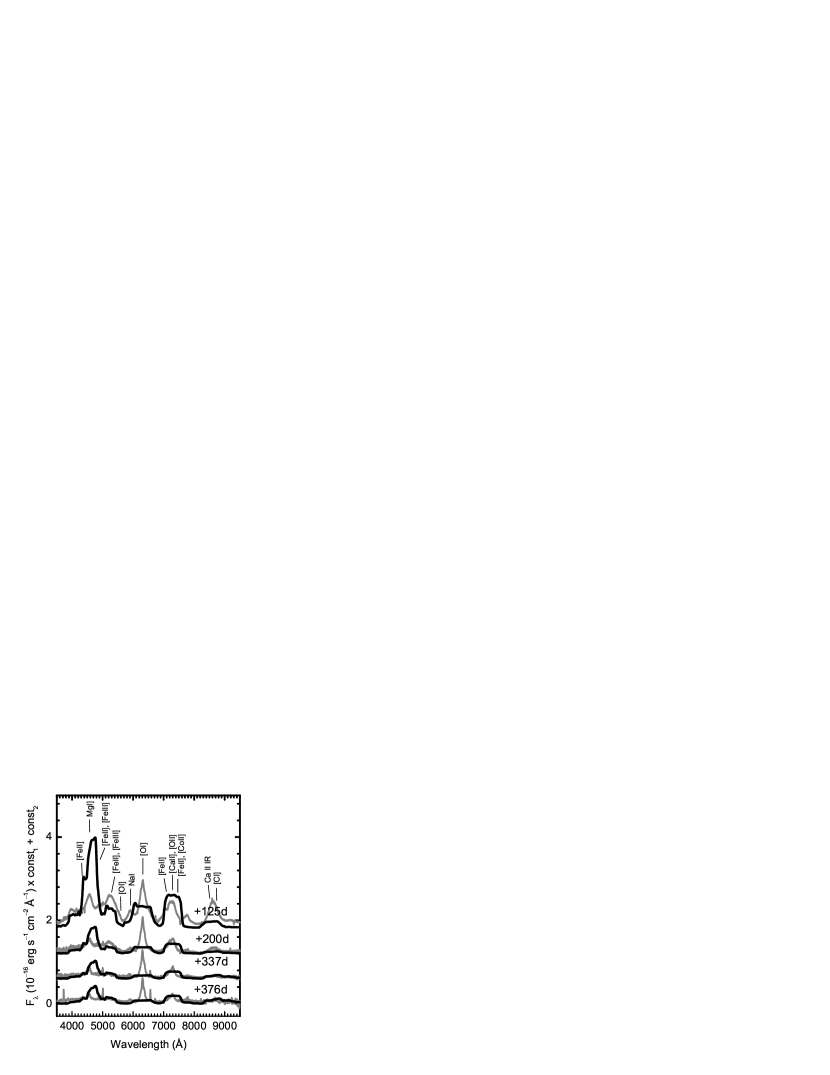
Figure 1: Synthetic spectra (black) for the original CO138E30 model as compared with the spectra of SN 1998bw (gray). For presentation, both the synthetic and observed spectra are multiplied by an arbitrary constant (const₁) and then vertically shifted upward by another factor (const₂). The amounts (const₁, const₂ in units of $10^{-16}$ erg s^-1 cm^-2 Å^-1) are as follows: +125^d (0.1, 1.8), +200^d (0.1, 1.2), +337^d (0.5, 0.6), and +376^d (1.0, 0.0). The mass of ⁵⁶Ni is $0.8M_{\odot}$.

With the time-dependent computational code, we first examine the synthetic spectra for the original spherical hypernova model CO138E30 (Iwamoto et al. 1998; Nakamura et al. 2001). The mass cut, i.e., the boundary between the collapsing core and the ejecta, chosen in the present work is deeper than the original, yielding the mass of ⁵⁶Ni $\sim 0.8M_{\odot}$ in order to roughly fit luminosities at the late phases (The original model with ⁵⁶Ni $\sim 0.4-0.6M_{\odot}$ is fainter than the late-phase observations; Nakamura et al. 2001). Figure 1 shows the temporal evolution of the synthetic spectra as compared with the observed ones. We next try to obtain better fits by changing the density structure below $v\mathrel{\hbox to0.0pt{\lower 4.0pt\hbox{\hskip 1.0pt$\sim$}\hss}\raise 1.0pt\hbox{$<$}}10,000$ km s^-1 and the abundance distribution throughout the ejecta (described below in more detail). The temporal sequence of the spectra of this ”modified” CO138E30 model is shown in Figure 2. The density structure and abundance distribution are shown in Figures 3 and 4, respectively.

The ”original” model has difficulties in reproducing both (a) line profiles in each single spectrum and (b) temporal evolution. As for the line profiles (a), elements in outer layers such as O and Mg produce synthetic lines with very wide, flat-topped profiles, while the observed [OI] 6300Å and MgI] 4570Å are narrow and sharply peaked. The flat-topped profile is the consequence of the distribution of emitting material with a central hole (See Figures 3 and 4a: O is distributed at $\mathrel{\hbox to0.0pt{\lower 4.0pt\hbox{\hskip 1.0pt$\sim$}\hss}\raise 1.0pt\hbox{$>$}}12,000$ km s^-1). Contrary to the observations, the synthetic [FeII] 5200Å blend is narrower than the synthetic [OI] 6300Å. This is a typical character of any spherically symmetric evolution-collapse-explosion model, as was pointed out by Mazzali et al. (2001). The problem in the temporal evolution (b) is that the ”original” CO138E30 model yields very rapidly fading lines [OI] 6300Å and MgI] 4570Å between the epochs $+125^{\rm d}$ and $+200^{\rm d}$ (Fig. 1).

The modified model (Fig. 2) is constructed so as to overcome these problems. The line profiles suggest that Fe (mainly synthesized as ⁵⁶Ni at the explosion) is on average distributed at higher velocities than hydrostatic burning products, e.g., O and Mg. The sharply peaked [OI] and MgI] lines can be accounted for if these lines are predominantly emitted at low velocity. In the one dimensional representation, a peculiar abundance distribution is therefore required: A high density O-rich core is added to the original CO138E30 model. It also helps to explain the more rapid decline of the [FeII] than the [OI] 6300Å and the MgI] 4570Å emission (Patat et al. 2001), since the contribution of higher velocity material becomes smaller as time goes by. Because deposition rate is larger in the modified model than in the original one, the mass of ⁵⁶Ni is smaller in the former, $M$(⁵⁶Ni) $\sim 0.6M_{\odot}$.

Another feature of the modified model is some mixing between the Fe-rich layer (originally at velocities at $\sim 8,000-12,000$ km s^-1) and the O-rich core (added at $\mathrel{\hbox to0.0pt{\lower 4.0pt\hbox{\hskip 1.0pt$\sim$}\hss}\raise 1.0pt\hbox{$<$}}8,000$ km s^-1). The observed [FeII] 5200Å and [CaII] 7300Å lines show mildly peaked profiles (though less sharply peaked than the [OI] and MgI]), suggesting that a small fraction of the Fe-rich materials are mixed downward into the low velocity O-rich core. The suggestion that (at least in a spherically symmetric representation) mixing is necessary was already made by Sollerman et al. (2000). Our model represents an even more unusual structure (from the point of view of 1D hydrodynamics), since the O-rich core is located at low velocities together with just a small fraction of Fe. This helps to keep the ionization of Fe as high as what is inferred from the observed spectra, although the usual mixing (Sollerman et al. 2000) with an Fe-dominated central region will lead to too low an ionization.

The mixing is also favored in view of the temporal evolution of each line intensity. Without any mixing, energy deposited by $\gamma$-rays and positrons into the O-rich region is all reprocessed into oxygen lines, predominantly into the [OI] 6300, 6363Å doublet. Therefore, the temporal evolution of [OI] 6300Å emission roughly traces the deposition rate, yielding too rapid fading of the line from $+125^{\rm d}$ to $+200^{\rm d}$ (Fig. 1). If other elements such as iron are mixed in, then the situation is different. Intensity of each line depends on contribution from others, which also depends on thermal condition within the nebula. In the materials composed with both iron and oxygen, the intensity ratio [FeII] 5200Å/[OI] 6300Å decreases rapidly with decreasing density, yielding larger relative intensity of [OI] 6300Å in more advanced epochs. Given that the sum of the intensities of these lines roughly follows the deposition rate, increasing relative importance of [OI] 6300Å with time yields the [OI] less rapidly fading than in the absence of any mixing.

The modified model (Figs. 3 and 4b) is constructed by mixing Fe from the Fe-rich layer downward into the O-rich core and compensate for it by mixing oxygen from the O-rich core into the Fe-rich layer. The same is also done for Ca. In addition, intensity of the [OI] 6300Å at the first epoch is further decreased by introducing clumping in the O-rich region. Regarding clumping, first introduced for SN 1998bw by Mazzali et al. (2001), the following facts give hints: (1) Without clumping [FeIII] is too strong at $\sim 4700$Å, which is not seen in the observations. (2) The intensity ratio of [CaII] 7300Å to CaII IR is too large in the original CO138E30 model. Therefore, we have introduced a filling factor of 0.1 throughout the ejecta The filling factor is kept unchanged at all epochs.

Comparing Figures 1 and 2, it is seen that the fit to the observed spectral sequence is very much improved. There are still some difficulty in reproducing the spectrum at $+125^{\rm d}$ (while it is much better than the original model). In addition to the strong [OI] 6300Å emission in the synthetic spectrum, MgI] 4570Å was also too strong at the first epoch (In Fig. 2, the mass fraction of Mg is reduced by a factor of 10 at the first epoch relative to the subsequent epochs). However, it may simply be that the density in the first epoch is too high to apply the nebular spectral computation (see §4). The present model is in a sense ad hoc, introducing peculiar elements distribution and density structure (i.e., O-rich core). We will show in §3 that this apparent peculiarity in one-dimensional representation can naturally be interpreted in the context of a two-dimensional model.

3 TWO DIMENSIONAL MODELS

3.1 Method and Models

We have developed a two-dimensional code, which is applicable to any two-dimensional distribution of density and abundances (including the distribution of the heating source ⁵⁶Ni). In the current version, axisymmetry along the $z$-axis (polar axis) and reflection symmetry on the equatorial plane are assumed. The included physics is the same with the one dimensional code. The difference between the one- and two-dimensional versions is in the treatment of the $\gamma$-ray deposition and the computation of the whole spectrum. The $\gamma$-ray deposition is solved as a two dimensional radiation transport problem using the Monte-Carlo Method. Ionization and NLTE thermal balance are solved in each mesh zone independently, since these processes take place locally as long as the optical depth is negligibly small. A synthetic spectrum is then computed for different orientations (divided uniformly into 10 degree angular zones), taking into account different Doppler shifts for different orientations.

We use as input the models presented in Maeda et al. (2002). These include spherical and aspherical explosions of a $16M_{\odot}$ He star, the core of a star of $M_{\rm ms}=40M_{\odot}$. Asphericity was generated assuming angle-dependent energy deposition, preferentially concentrated toward the polar direction, at the center of the collapsing core (See Maeda et al. (2002) for details).

The models we explore in this paper are listed in Table 1. The distributions of density and of a few selected elements in the homologous expansion phase are presented in Figure 5. We examine models with various degree of asphericity defined by the parameter BP. The value of BP is the axial ratio of the initial aspherical energy injection. See Maeda et al. (2002) for details (their parameter $\alpha/\beta$ is the same as BP). The models correspond to those of Maeda et al. (2002) as follows: BP16 (A), BP8 (C), BP2 (E), and a spherical model BP1 (F). In the present work, we add an additional model (BP4) which has an asphericity intermediate between models BP8 and BP2, by repeating the calculations of Maeda et al. (2002) but with a different asphericity parameter.

As seen in Table 1, we generate a series of models with various kinetic energy by artificially multiplying the velocities at any points in the ejecta by a factor $f_{V}$. The factor $f_{V}$ is taken as a parameter, ranging from 0.7 to 1.9. For each model specified by the parameters BP and $f_{V}$, the masses of oxygen ($M_{\rm O}$) and ⁵⁶Ni in the ejecta are changed by hand in order to obtain a good fit to the intensities of the [OI] 6300Å, 6363Å and the [FeII] 5200Å (see §3.2 for details). The kinetic energy in the ejecta is scaled as $E_{\rm K}\propto M_{\rm ej}{f_{V}}^{2}$, where $M_{\rm ej}$ is the ejecta mass, mainly oxygen, obtained by spectral fitting. Because of the procedure, the oxygen mass and therefore the kinetic energy are different from the original values ($M_{\rm O}\sim 8M_{\odot}$ and $E_{51}\sim 10$).

Computing nebular spectra for these models, we obtain synthetic spectra resulting from various energies and ejecta masses (and thus progenitor masses). Summarizing, a spectrum of a particular model is specified by three parameters: the asphericity BP, the velocity scale $f_{V}$ (which gives the energy in the ejecta), and the orientation to the observer $\theta$ (defined as the angle between the polar and the observer direction).

3.2 Overall Spectra and Model Construction

We compare our synthetic spectra for the two dimensional, aspherical supernovae with the spectra of SN 1998bw (Patat et al. 2001) obtained at 125, 200, 337, and 376 days after B maximum. We especially focus on the +337^d spectrum, since the epoch is sufficiently late that the contribution of allowed Fe transitions (which are not included in the model) on the [FeII] blend near 5200Å is likely negligible (see §4.5.1).

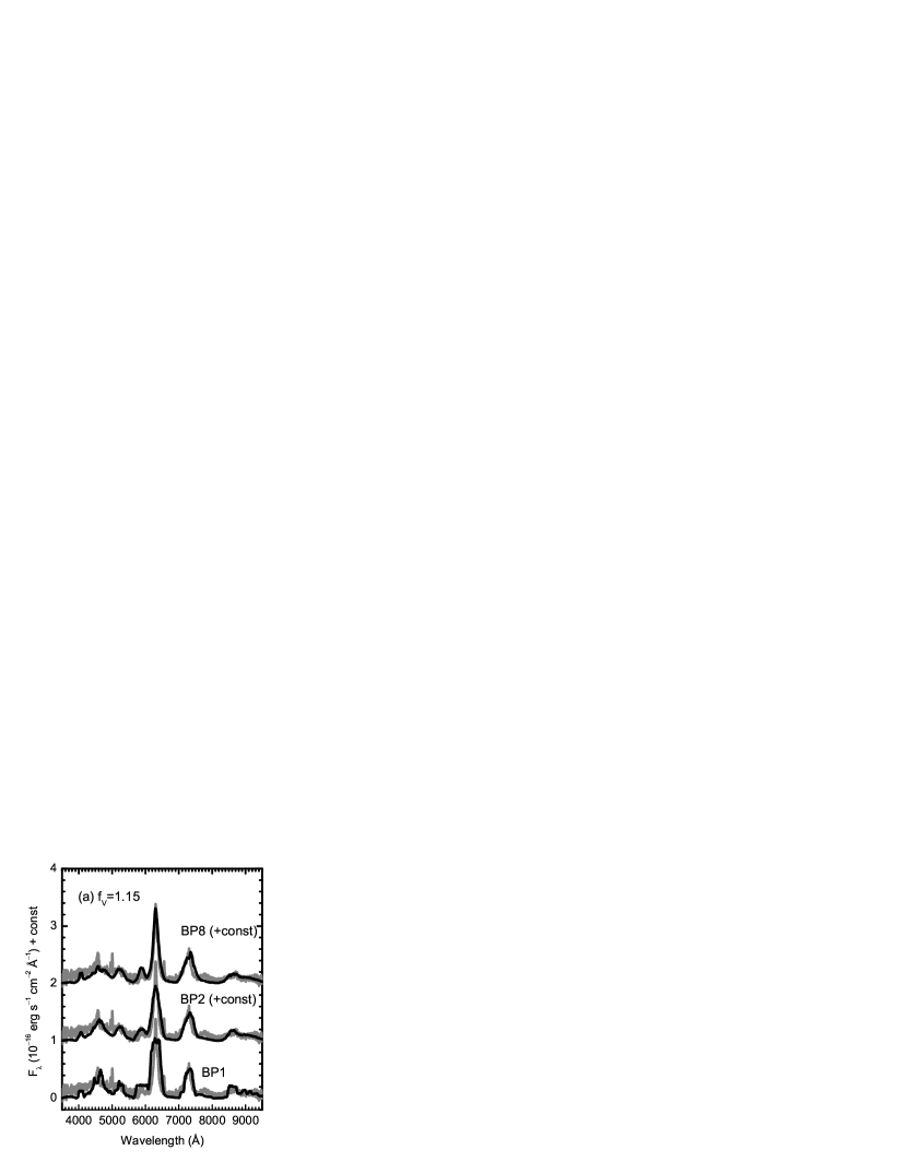
Figure 6: Examples of synthetic spectra (black lines) as compared with the spectrum of SN 1998bw at 337 days after the maximum light (gray lines). Shown here are Models BP8, BP2, and BP1 with (a) $f_{V}$=1.15 and $\theta=30^{\rm o}$ and with (b) $f_{V}$=1.6 and $\theta=30^{\rm o}$. The spectra of BP8 and BP2 are shifted vertically for presentation (+2 and +1 $\times 10^{-16}$ erg s^-1 cm^-2 Å^-1) for BP8 and BP2, respectively).

Figure 6 shows examples of the synthetic spectra with a viewing angle $\theta=30^{\rm o}$. The synthetic spectra are very much improved for the aspherical model, especially for the one with BP=8 and $f_{V}$ =1.15, compared to the spherical hydrodynamic explosion models (either the original CO138E30 in Fig. 1 or models BP1 in Fig. 6). The sharply peaked MgI] 4570Å, [OI] 6300, 6363Å, and NaI 5900Å, as well as the broad [FeII], are naturally explained. Indeed, the fit by the aspherical model BP8 ($f_{V}$=1.15) is as good as the one by the one dimensional ”modified” CO138E30 model. The masses of oxygen and ⁵⁶Ni are determined so as to obtain the correct line strengths (at +337days) in the two-dimensional models. This is done by reducing/increasing the density uniformly throughout either the ⁵⁶Ni or O rich region (see below). Therefore, each line profile is not sensitively affected by this procedure but results from the explosion model itself.

Figure 6 also shows how different kinetic energy and asphericity affect the synthetic spectrum. For example, we can definitely rule out the model BP2 with $f_{V}$=1.6 for SN 1998bw, since the [OI] 6300Å line is too broad and its shape is less sharply peaked than in the observation. We discuss the profiles of each line in more detail in §3.3 and in the Appendix. The selection of models acceptable for SN 1998bw is discussed in §3.4.

Because the intensities of the [FeII] 5200Å and the [OI] 6300Å are well defined in the observation, they can be used to constrain the masses of iron (mostly the product of ⁵⁶Ni decay) and oxygen. These are model-dependent as the combination of mass and energy gives the average density, which in turn gives the deposition rate. For example, we find that the original hydrodynamic models (where $M_{\rm O}\sim 8M_{\odot}$ and $E_{51}\sim 10$) yield too strong [OI] emission relative to [FeII] 5200Å. Therefore $M_{\rm O}$ should be reduced to fit the line ratio correctly (e.g., $M_{\rm O}\sim 4.7M_{\odot}$ in model BP1, $f_{V}$=1). In the current study, we have uniformly reduced densities in oxygen-dominated regions, and therefore $M_{\rm O}$, until we obtained the correct intensity ratio [OI] 6300Å/[FeII] 5200Å at day +337. The mass of ⁵⁶Ni is also constrained by the total luminosity in the observed spectrum. Therefore, we also changed the mass of ⁵⁶Ni (densities in ⁵⁶Ni dominated regions) until we obtained the correct luminosity at $+337^{\rm d}$. The masses $M$(⁵⁶Ni) and $M_{\rm O}$ consistent with the observed flux at $+337^{\rm d}$ are thus derived for all the models as listed in Table 1. Note that a model with larger $f_{V}$ has lower density and smaller deposition rate, and therefore needs larger $M_{\rm O}$ and $M$(⁵⁶Ni) to fit the observed intensities. This is the reason the energy $E_{\rm K}$ in the larger $f_{V}$ models is larger than expected from the simple scaling $E_{\rm K}\propto{f_{V}}^{2}$, because the mass of the ejecta needed is also larger for larger $f_{V}$.

3.3 Emission Lines

Dependencies of line profiles of the [FeII] blend 5200Å, the [OI] 6300, 6363Å doublet, the MgI] 4570Å, and the [CaII] 7291, 7324Å on the three parameters, $f_{V}$, $\theta$, and BP are described in Appendix in detail. Here we give a very brief summary.

• $f_{V}$: Irrespective of $BP$ and $\theta$, larger $f_{V}$ yields broader profiles for every line.

• $\theta$: The profile depends on whether the emitting element is explosive burning product (Fe and Ca) or hydrostatic product (O and Mg). For the former, the line is broader for smaller $\theta$. For the latter, the dependence is in the opposite sense.

• BP: For explosive burning products, larger BP yields a broader [narrower] line if $\theta$ is small [large]. For hydrostatic products, the dependence is in the opposite sense.

3.4 SN 1998bw: Two Dimensional Approach

In this section, we discuss which models are acceptable for SN 1998bw, according to each line profile (§3.3 and Appendix). On the basis of the selected models, we further seek for conditions that may yield better fits to the observations in a manner similar to what was done for the 1D model (by introducing mixing and clumping; §2.2).

Figure 7 illustrates how the model parameters are constrained by the observations. A fit is judged by the following rules. For the [FeII] 5200Å, it is checked if the width of the blend is consistent with the observed value. The region of acceptance is larger for $\theta=0^{\rm o}$ than $\theta=30^{\rm o}$, since the former results in a broader profile. For the [OI] 6300Å, if a model fits well the line wings and does not produce a double-peaked emission line, it is regarded to be acceptable. The fit to the MgI] 4570Å is not included, because the MgI] gives the same constraints as the [OI] 6300Å lines, but with less accuracy.

The fit to the [CaII] 7300Å line is uncertain. In a strict sense, no present model, either spherical or aspherical, gives acceptable fits, since the observed line center is shifted blueward relative to the models. See Appendix for details. Here, we tentatively regard a fit as acceptable if the emission at the blue wing is consistent with the observation. By doing this, models producing a doubled-peaked or a too broad flat-topped profile are excluded. There are several ways to shift the line center or to depress the emission in the red, as we will discuss in §4. The region of acceptance for [CaII] 7300Å moves to more aspherical and more energetic models (yielding a broader Ca line) for larger viewing angle $\theta$ (yielding a narrower Ca line), so that these two effects compensate one another.

Figure 7 shows that both the [FeII] 5200Å and the [OI] 6300Å are explained by highly aspherical (${\rm BP}\mathrel{\hbox to0.0pt{\lower 4.0pt\hbox{\hskip 1.0pt$\sim$}\hss}\raise 1.0pt\hbox{$>$}}8$), energetic models ($f_{V}\mathrel{\hbox to0.0pt{\lower 4.0pt\hbox{\hskip 1.0pt$\sim$}\hss}\raise 1.0pt\hbox{$>$}}1$) viewed in a direction close to the pole ($\theta\mathrel{\hbox to0.0pt{\lower 4.0pt\hbox{\hskip 1.0pt$\sim$}\hss}\raise 1.0pt\hbox{$<$}}30^{\rm o}$). Viewing angles $\theta\gg 30^{\rm o}$ do not produce an acceptable fit to [OI] 6300Å. Also, the width of the [OI] line sets an upper limit for $f_{V}$ (and therefore on the energy), since models with $f_{V}\mathrel{\hbox to0.0pt{\lower 4.0pt\hbox{\hskip 1.0pt$\sim$}\hss}\raise 1.0pt\hbox{$>$}}1.6$ produce too broad [OI] emission. If we include [CaII] 7300Å in the fit despite the large uncertainty, $\theta\sim 30^{\rm o}$ is preferred, since highly aspherical and energetic models produce double peaked or too broad [CaII] emission if viewed at $\theta\sim 0^{\rm o}$ or even at $\theta\sim 15^{\rm o}$ as mentioned in Maeda et al. (2002) (who did not include the [CaII] in the model). If only the [FeII], [OI] (and MgI]) are considered in the fit, the fit by models with $\theta=15^{\rm o}$ is as nice as $\theta=30^{\rm o}$. The [CaII] 7300Å feature is complicated and therefore needs further study to understand its nature (§4).

Next, we examine the temporal spectral evolution of one of the acceptable models (BP8, $f_{V}$=1.15, and $\theta=30^{\rm o}$). This is shown in Figure 8a. Additionally, Figure 8b shows model BP8 with $f_{V}$=1.6 and $\theta=30^{\rm o}$. The latter model is not regarded as ”acceptable” because the [OI] 6300Å line is too broad if it is normalized at the emission peak (see Appendix). The fit to the wings of the [OI] emission, however, is not bad, therefore the fit is marginal.

For SN 1998bw, this is the first attempt to check the consistency of a theoretical model by time-dependent computations. Figure 8 shows that both models have difficulty in reproducing the slowly fading [OI] 6300Å and MgI] 4570Å from $+125^{\rm d}$ to $+200^{\rm d}$, a similar problem also encountered for the one dimensional model CO138E30.

As done in §2, we have attempted to obtain better fits, by introducing mixing and clumping. Guided by the 1D model, we have tried to simulate these effects. First, mixing between the Fe-rich region and the O-rich region is taken into account by changing a fraction of O in the O-rich region into Fe and Ca. Second, we have also increased the mass of C in the O-rich region since the synthetic feature near 8500Å shows a deficiency of [CI] (Fig. 8). Obviously hydrodynamic explosion models, either one or two dimensional, yield a mass fraction of carbon in the O-rich region insufficiently small to fit the [CI] line strength (see also Fig. 1). Finally, we have introduced filling factors to simulate clumping both for the Fe-rich and the O-rich regions.

These parameters for mixing and clumping are set so as to obtain a fit as nice as possible. Figure 9 shows the spectra of the ”modified” 2D models. The parameters for the modification are as follows. For the BP8, $f_{V}$=1.15 model, 3%, 1%, and 10% of O in the O-rich region are changed to Fe, Ca, and C, respectively. Then filling factors of 0.1 and 0.2 are introduced in the Fe- and O-rich regions, respectively. For the BP8, $f_{V}$=1.6 model, 1.5%, 1%, and 10% of O in the O-rich region are changed to Fe, Ca, and C, respectively. Then filling factors of 0.05 and 0.1 is introduced in the Fe- and O-rich regions, respectively.

Comparing Figures 8 and 9 shows that the fit is improved very much by introducing mixing and clumping. The modified 2D models match the observed spectra as nicely as the modified 1D model (see Fig. 9). The main deference between the modified 1D model and the 2D model is that the modified 1D model is very different from the original CO138E30 model. The modification yielded line profiles different from the original model. The distributions of density and abundances in this model are inconsistent with the results of ”1D” explosion hydrodynamics. In the 2D model, on the other hand, the distribution of density and abundances are based on the aspherical explosion model. The changes due to the modification of the abundance distribution and the introduction of mixing and clumping, which may naturally occur, are small. This does not sensitively affect the line profiles.

4 Summary and Discussion

4.1 Summary

We have revisited the nebular spectra of SN 1998bw, using one- and two-dimensional nebular spectrum synthesis codes. Compared with previous works (1D models by Sollerman et al. 2000 and Mazzali et al. 2001, and a 2D model by Maeda et al. 2002), we have extended the analysis in the following points. In the 1D model, we have tried to construct a model which explains the temporal evolution of the spectra of SN 1998bw from +125^d to +376^d. The distribution of the density and elements of the model (the modified CO138E30) is far from what is expected from 1D spherically symmetric explosion models. We have further computed 2D synthetic spectra of the aspherical explosion models of Maeda et al. (2002). These models show that an aspherical explosion scenario naturally explains the late-phase spectra of SN 1998bw. In the 2D model, we have extended the analysis of Maeda et al. (2002), including more realistic computations and more detailed comparison with the observations.

As for the one-dimensional model, our main results are as follows. (1) The original CO138E30 model for SN 1998bw (obtained by fitting the early phase observations up to $\sim 2$ months) is not consistent with the late-phase spectra. (2) A high-density O-rich core below $\sim 8,000$ km s^-1 is necessary to explain the sharply-peaked [OI] 6300Å, 6363Å doublet profile. (3) At the same time, a large amount of ⁵⁶Ni (which decays into Fe) should be located at $v\mathrel{\hbox to0.0pt{\lower 4.0pt\hbox{\hskip 1.0pt$\sim$}\hss}\raise 1.0pt\hbox{$>$}}8,000$ km s^-1 to reproduce the large ratio between the widths of [FeII] 5200Å and [OI] 6300Å. The above three features are not accounted for by any spherically symmetric evolution-collapse-explosion calculations. (4) Heavy elements such as Fe and Ca are likely mixed into the O-rich region, and vice versa. Namely, O, Fe, and Ca do not occupy completely separated layers. (5) Clumping is important both in O-rich and Fe-rich regions.

In the context of the two-dimensional models, our results can be summarized as follows. (1) The [FeII] 5200Å and the [OI] 6300Å lines are naturally reproduced by (some) aspherical models, confirming the suggestion of Maeda et al. (2002). (2) The profile of the MgI] 4571Å gives additional support to the aspherical model for SN 1998bw. The analysis of the [CaII] profile demonstrates, however, that the present models are still not perfect. (3) Examining a wide parameter range, we have shown that nebular spectra of SN 1998bw indeed require a hyper-energetic explosion (see also §4.2). (4) Similar to the 1D model, mixing and clumping are at least partly responsible for the slow spectrum evolution from $+125^{\rm d}$ to $+200^{\rm d}$.

4.2 The Nature of SN 1998bw

According to the present model, we can infer the nature of SN 1998bw. It was an highly aspherical explosion (BP $\sim 8$) viewed at $0^{\rm o}<\theta\mathrel{\hbox to0.0pt{\lower 4.0pt\hbox{\hskip 1.0pt$\sim$}\hss}\raise 1.0pt\hbox{$<$}}30^{\rm o}$. The viewing angle is consistent with the off-axis model ($16^{\rm o}\mathrel{\hbox to0.0pt{\lower 4.0pt\hbox{\hskip 1.0pt$\sim$}\hss}\raise 1.0pt\hbox{$<$}}\theta\mathrel{\hbox to0.0pt{\lower 4.0pt\hbox{\hskip 1.0pt$\sim$}\hss}\raise 1.0pt\hbox{$<$}}36^{\rm o}$) explaing properties of prompt gamma ray emission of GRB 980425 associated with SN 1998bw (Yamazali, Yonetoku, & Nakamura 2003). The kinetic energy in the explosion models giving the best fits was $E_{51}\sim 8-12$, mass of ⁵⁶Ni $M$(⁵⁶Ni) $\sim 0.4-0.5M_{\odot}$), and mass of oxygen in the ejecta $M_{\rm O}\sim 5-6M_{\odot}$. The mass of oxygen would correspond to a CO core of $\sim 9-10M_{\odot}$ and to a He core of $\sim 11-12M_{\odot}$, which is evolved from a star with $M_{\rm ms}\sim 30-35M_{\odot}$. The argument assumes the central remnant is a $4M_{\odot}$ black hole, which could be larger if a larger fraction of the O-dominated layer is accreted onto the black hole (e.g., MacFadyen & Woosley 1999; Maeda & Nomoto 2003b).

Here we would like to discuss the uniqueness of the model. A fit to each line is used to restrict a possible range in the parameter space (BP, $f_{V}$, and $\theta$). Because the line shapes of different elements depend on the parameters differently (see §3.3 and §3.4), the combination of fits to several lines is useful to narrow down the parameter space (Fig. 7). Once these parameters are given, then the masses of ⁵⁶Ni and ejecta mass are derived based on the line intensities, and therefore $M$(⁵⁶Ni), $M_{\rm ejecta}$, and $E_{\rm K}$ are determined rather uniquely. The above model is derived including a qualitative fit to [CaII] 7300Å, which is not very certain in the present study (see §3.4 and §4.5.2). If we omit this line, and use only the [OI] 6300Å, MgI] 4570Å, and [FeII] 5200Å, then the degeneracy is not completely resolved (Fig. 7). For example, assuming $\theta=30^{\rm o}$ the models with BP $\mathrel{\hbox to0.0pt{\lower 4.0pt\hbox{\hskip 1.0pt$\sim$}\hss}\raise 1.0pt\hbox{$>$}}8$ and $1\mathrel{\hbox to0.0pt{\lower 4.0pt\hbox{\hskip 1.0pt$\sim$}\hss}\raise 1.0pt\hbox{$<$}}f_{V}\mathrel{\hbox to0.0pt{\lower 4.0pt\hbox{\hskip 1.0pt$\sim$}\hss}\raise 1.0pt\hbox{$<$}}1.45$ ($6\mathrel{\hbox to0.0pt{\lower 4.0pt\hbox{\hskip 1.0pt$\sim$}\hss}\raise 1.0pt\hbox{$<$}}E_{51}\mathrel{\hbox to0.0pt{\lower 4.0pt\hbox{\hskip 1.0pt$\sim$}\hss}\raise 1.0pt\hbox{$<$}}16$) are acceptable. For smaller $\theta$, the range is even larger, while values $\theta\sim 0^{\rm o}$ are disfavored because they do not even give a qualitatively acceptable fit to [CaII] 7300Å. The models can be further constrained by fitting early-phase observations, i.e., light curve and spectra (K. Maeda, in preparation).

We regard the above mass of oxygen and especially the kinetic energy in the two-dimensional model as lower limits of those in the real ejecta for the following reason. Although we have computed a spectrum based on realistic explosion models, it is not certain that the models really give a good representation of material at velocities $\mathrel{\hbox to0.0pt{\lower 4.0pt\hbox{\hskip 1.0pt$\sim$}\hss}\raise 1.0pt\hbox{$>$}}10,000$ km s^-1 since they emit little at the late-phases. Our explosion models contain material up to $\sim 15,000-25,000$ km s^-1 for $f_{V}=1-1.6$, above which the density drops very rapidly as a function of radius and therefore was not traced by the two-dimensional explosion calculations. However, the early-phase spectra suggest there is material up to $\sim 40,000$ km s^-1 which carries a substantial fraction of the total kinetic energy (Nakamura et al. 2001; see also Mazzali et al. 2000). Although the origin of such material is not clear, its existence suggests that the total kinetic energy should be larger than that of the present two-dimensional model.

In any case, the lower limit of the kinetic energy $E_{51}\mathrel{\hbox to0.0pt{\lower 4.0pt\hbox{\hskip 1.0pt$\sim$}\hss}\raise 1.0pt\hbox{$>$}}10$ is much larger than the typical value $E_{51}\sim 1$. Less energetic models do not fit the observed nebular spectra of SN 1998bw, especially at [FeII] 5200Å.

Also, our models suggest that the ejecta is likely very clumpy and that nucleosynthetically different layers are mixed. This is necessary to explain the spectral evolution, especially the slow fading of [OI] 6300Å and MgI] 4570Å between $+125^{\rm d}$ and $+200^{\rm d}$. The amount of mixing is small and may well be explained in the context of Rayliegh-Taylor or shear instabilities between the O-rich and the Fe-rich region (for Fe and Ca) and between the O-rich region and the C layer above it (for C). Such mixing processes are believed to take place in core-collapse supernovae (e.g., the earlier than expected detection of X-rays and $\gamma$-rays from SN 1987A: Dotani et al. 1987; Sunyaev et al. 1987; Matz et al. 1988: see e.g., Kifonidis et al. 2000 for recent simulations). Also, aspherical explosions are suggested to boost the efficiency of the mixing (Nagataki, Shimizu, & Sato 1998). While we have introduced a rather large C abundance (10%) in the O-rich region, both C and O are hydrostatic burning products, and therefore additional mixing could also operate in hydrostatic evolution stages. This may be naturally explained by rotationally induced mixing (e.g., Iwamoto et al. 2005), since the large asphericity at the explosion implies that the progenitor star was a very rapid rotator.

4.3 Implications for the Light Curve

We derived a mass of ⁵⁶Ni, $M$(⁵⁶Ni) $\sim 0.4M_{\odot}$ in the two dimensional model. This is consistent with the results of previous work (e.g., Nakamura et al. 2001). The distribution of ⁵⁶Ni in our model is characterized by a large amount of ⁵⁶Ni in the high velocity outer region, and a small fraction in the inner high density region. The distribution will affect the shape of the light curve. Figure 10 shows the evolution of the luminosity deposited by $\gamma$-rays and positrons, i.e., optical light curve applicable after $\sim 50-100$ days. At least qualitatively, the 2D models are favored over the original 1D CO138E30 model, thanks to the presence of ⁵⁶Ni at high velocities and the high density core at low velocities (Maeda et al. 2003a). Computation of 2D light curves from the explosion to the late-phases on the basis of the two dimensional models will be another check of the validity of the models (see also Höflich, Wheeler, & Wang 1999).

4.4 Notes for Future Observations

Our suggestion that hypernovae are aspherical explosions may further be able to be confirmed by future observations. First, we suggest to take late-phase near-infrared (NIR) spectra of supernovae with SN 1998bw-like early-phase spectra, as has been done for SNe Ia (e.g., Höflich et al. 2004). In the NIR, a [FeII] line is more isolated than in the optical band, making the effect of the orientation easier to see.

It is also interesting to examine the [OI] 6300Å profile in other hypernovae and SNe Ib/c to investigate the effect of the viewing angle. Recently, Kawabata et al. (2004) reported the detection of the double-peaked [OI] 6300Å in a spectrum of SN 2003jd at $\sim 1$ year after the discovery. Mazzali et al. (2005) interpreted it as a SN 1998bw-like event, as suggested from early-phase spectroscopy, but viewed from the equatorial direction. Although the sample is small in number for hypernovae, late-phase spectra such as those published for SNe Ib/c by Matheson et al. (2001) would allow statistical studies to constrain the explosion energy and the asphericity of SNe Ib/c.

4.5 Remaining Problems

4.5.1 The Spectrum at $+125^{\rm d}$

One of the major advances in the present study is the time-dependent computations of the nebular spectra of SN 1998bw. The model derived at the spectrum at +337^d gives nice fits to the sequence of the spectra after +200^d. However, at the first epoch +125^d, some deviation from the observations still exists especially in the luminosity of the [OI] 6300, 6363Å doublet, even though we have tried to fix this by introducing mixing and clumping. Others are the strong [FeII] and [FeIII] between 4000Å and 5000Å  and the strong MgI] 4570Å and [OI] 5577Å in the model. They may simply be due to inappropriate treatment of the first epoch +125^d in our computation since at this epoch the ejecta density is still high and the nebular representation may not totally be a good approximation. Temporal evolution of the intensity of the [OI] 6300Å changed around $+125^{\rm d}$ (Patat et al. 2001), implying that at this epoch the ejecta are still in the transition from the photospheric phase to the nebular phase. For example, the observationally strong OI 7800Å implies that allowed transitions may be dominant in some wavelength ranges.

Because of the possible presence of emission lines of some strong allowed Fe II transitions, the identification of the 5200Å feature as the blend of forbidden lines only may be uncertain. Axelrod (1980) computed optical depths of the strongest allowed Fe II lines near 5200Å for a model SN Ia nebula at days 87 and 264 to be of the order of 10 and 0.1, respectively. Given the larger ratio $E_{\rm K}/M$(⁵⁶Ni) in our models for SN 1998bw than for SNe Ia, the optical depths will be even smaller. Rough estimates suggest that a few lines may have optical depth of order unity at the first epoch ($+125^{\rm d}$). Therefore, at this epoch the contribution of the allowed Fe II lines and related radiation transfer effects, e.g., line scattering, may affect (but probably not dominate) the shape of the 5200Å feature. At the same time, the same estimate shows that the optical depths of the allowed Fe lines will be very small (of the order of 0.1 or less) at $+200^{\rm d}$ and thereafter, justifying the assumption that the contribution of the allowed lines and radiation transfer effects are negligible. See also Maeda et al. (2002) for a detailed discussion of the identification of the 5200Å feature as the forbidden lines.

As for the MgI] 4570Å, the line emissivity is quite sensitive to the treatment of the photoionization radiation field because of its low ionization threshold (Houck & Fransson 1996; Kozma & Fransson 1998a), while the ionization by UV photons is not included in our present spectrum synthesis calculations (See also, e.g., Sollerman et al. 2004 for the effect of photoionization). This could partly be a reason of our failure in fitting the temporal evolution of the MgI] 4570Å luminosity, since the effect is expected to be stronger at earlier epochs. We plan to extend our code to allow better treatment at such relatively early epochs.

4.5.2 Peculiar [CaII] Emission

The final question we should answer in the future concerns the origin of the peculiar [CaII] 7300Å emission. As mentioned in Appendix, the model spectra are too red. It is interesting that another hypernova, SN 2002ap, shows the [CaII] 7300Å line exactly at the correct position (Kawabata et al. 2002; Leonard et al. 2002; Wang et al. 2003; Foley et al. 2003). The blueshift of the line in SN 1998bw seems to be unique.

The feature is a complex blend and therefore it is difficult to clarify the reason of the failure in the model. With this caveat taken in mind, we speculate possibilities which may explain the discrepancy. The problem is possibly related to the distribution of Ca. There are at least two possibilities to reconcile the problem. First, the distribution of Ca may be similar to O, rather than Fe. It will then be challenging to the theory of explosive nucleosynthesis. Another possible interpretation would be that SN1998bw may have asymmetry even between the two hemispheres. If we look at the event from the hemisphere with the larger kinetic energy, the center of the Ca distribution would be blue shifted. This should however also apply to [FeII] 5200Å, which does not seem to show the shift. The significantly blended nature of [FeII] 5200Å may wash that signal away. In this context, SN2002ap would be an explosion in which the degree of this asymmetry is small or the viewing orientation is relatively large. This is an interesting possibility, and we will pursue this issue in the future. The above two possibilities could be resolved by examining a number of hypernova late-phase spectra. In our interpretation, the sample contains hypernovae with various viewing angles, then the two different Ca distributions – oxygen-like or iron-like – should give different statistics.

Appendix A Emission Line Profiles

A.1 [FeII] 5200Å

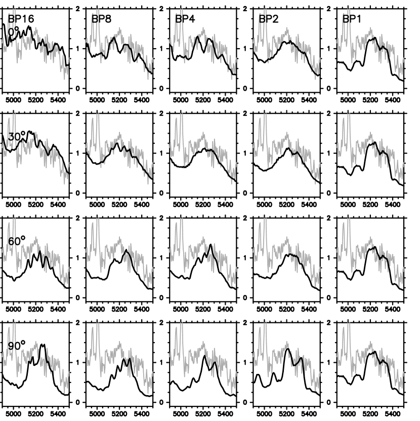
Figure 11: The synthetic spectra of the 2D models around 5200Å (black lines) as compared with the observed one of SN 1998bw at 337 days after the B maximum (gray lines). The synthetic spectra are mainly contributed by [FeII]. The models are those with $f_{V}=1.6$. Shown here are BP16, 8, 4, 2, 1 (from left to right) and $\theta=0,30,60,90^{\rm o}$ (from top to bottom).

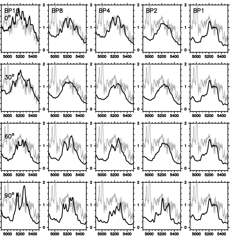
Figure 12: The same with Fig. 11 ([FeII] 5200Å), except the model parameter $f_{V}=1.15$.

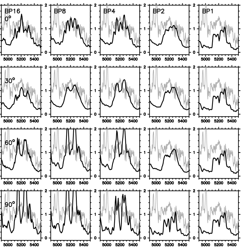
Figure 13: The same with Fig. 11 ([FeII] 5200Å), except the model parameter $f_{V}=0.7$.

Figures 11, 12, and 13 show how the shape of the [FeII] blend at 5200Å depends on the degree of asphericity and the observer direction. The dependence on the kinetic energy can also be seen by comparing Figures 11 ($f_{V}$=1.6), 12 ($f_{V}$=1.15), and 13 ($f_{V}$=0.7).

The dependencies can be summarized as follows. (1) For a given asphericity, a smaller viewing angle $\theta$ leads to a broader feature (with the obvious exception of the spherically symmetric models). (2) Larger asphericity leads to a broader [narrower] feature for small [large] $\theta$. (3) Larger kinetic energy leads to a broader feature irrespective of the degree of asphericity and orientation.

The above dependencies can be understood from the distribution of ⁵⁶Ni (Fe) in Figure 5. The distribution is elongated in the polar direction in the aspherical models. Larger asphericity leads to higher velocities in the polar direction and smaller ones in the equatorial direction. If the energy is larger, the velocity in all directions becomes larger. These characters of the ⁵⁶Ni distribution explain the dependence of the [FeII] feature on various parameters.

The observed broad 5200Å emission can be explained if the asphericity is large, the energy is large, and the viewing angle $\theta$ is small ($\theta\mathrel{\hbox to0.0pt{\lower 4.0pt\hbox{\hskip 1.0pt$\sim$}\hss}\raise 1.0pt\hbox{$<$}}30^{\rm o}$). For example, Figure 11 shows that for these very energetic models ($f_{V}$=1.6), the synthetic [FeII] 5200Å is as broad as the observed one for BP $\mathrel{\hbox to0.0pt{\lower 4.0pt\hbox{\hskip 1.0pt$\sim$}\hss}\raise 1.0pt\hbox{$>$}}2$ given $\theta\mathrel{\hbox to0.0pt{\lower 4.0pt\hbox{\hskip 1.0pt$\sim$}\hss}\raise 1.0pt\hbox{$<$}}30^{\rm o}$. For less energetic models, the criterion is tighter: For $f_{V}$=1.15, BP $\mathrel{\hbox to0.0pt{\lower 4.0pt\hbox{\hskip 1.0pt$\sim$}\hss}\raise 1.0pt\hbox{$>$}}8$ is necessary to produce the broad feature. For $f_{V}$=0.7, the synthetic [FeII] 5200Å is never as broad as the observed one, even if the asphericity BP is very large. Note also that if both the energy and the asphericity are extremely large (e.g., $f_{V}$=1.6 and BP=16), the synthetic feature is too broad.

A.2 [OI] 6300, 6363Å

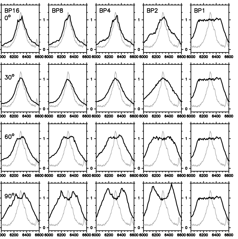
Figure 14: The synthetic spectra of the 2D models around 6300Å (black lines) as compared with the observed one of SN 1998bw at 337 days after the B maximum (gray lines). The synthetic spectra are predominantly contributed by [OI] 6300Å and 6363Å. The models are those with $f_{V}=1.6$. See the caption of Fig. 11 for the meanings of each panel.

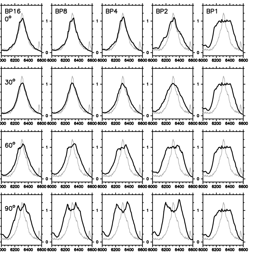
Figure 15: The same with Fig. 14 ([OI] 6300Å and 6363Å), except the model parameter $f_{V}=1.15$.

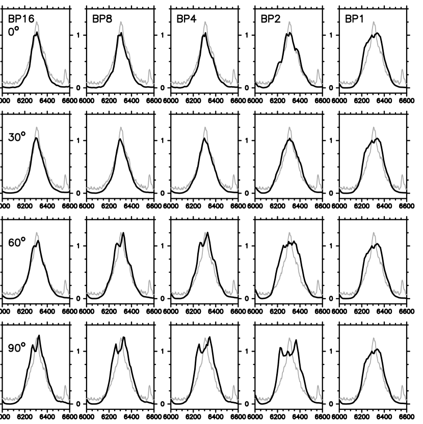
Figure 16: The same with Fig. 14 ([OI] 6300Å and 6363Å), except the model parameter $f_{V}=0.7$.

The dependence of the [OI] 6300, 6363Å doublet profile on various parameters is shown in Figures 14 – 16. The observed sharply-peaked profile with extended wings again favors highly aspherical models (BP16 or BP8) viewed from a direction close to the pole ($\theta\mathrel{\hbox to0.0pt{\lower 4.0pt\hbox{\hskip 1.0pt$\sim$}\hss}\raise 1.0pt\hbox{$<$}}30^{\rm o}$). In addition, the narrow [OI] 6300Å sets constraint on the model in a different way from the way the [FeII] 5200Å line does. For the less energetic models ($f_{V}$=0.7), all the aspherical models (BP = 2 – 16) give nicely peaked profiles if viewed near the pole. For $f_{V}$=1.15, larger BP (BP $\mathrel{\hbox to0.0pt{\lower 4.0pt\hbox{\hskip 1.0pt$\sim$}\hss}\raise 1.0pt\hbox{$>$}}4$) is required. Furthermore, for $f_{V}$=1.6, the synthetic [OI] 6300Å is broader than the observations, even for small viewing angles.

The sharply-peaked [OI] profile is produced by the edge-on view of a disk-like oxygen distribution. The model predicts a double-peaked profile if viewed near the equator as shown in Figures 14 – 16 for large $\theta$. A spherical explosion model like CO138E30 produces a flat-topped profile because of the central hole in oxygen distribution (at $\sim 10,000$ km s^-1 for the kinetic energy $E_{51}=30$; Figs. 4a and 5), which does not fit well the observations, irrespective of the total kinetic energy. This is especially evident in the larger kinetic energy model ($f_{V}$ $\mathrel{\hbox to0.0pt{\lower 4.0pt\hbox{\hskip 1.0pt$\sim$}\hss}\raise 1.0pt\hbox{$>$}}1$) which produces very broad [OI] 6300Å emission.

A.3 MgI] 4570Å

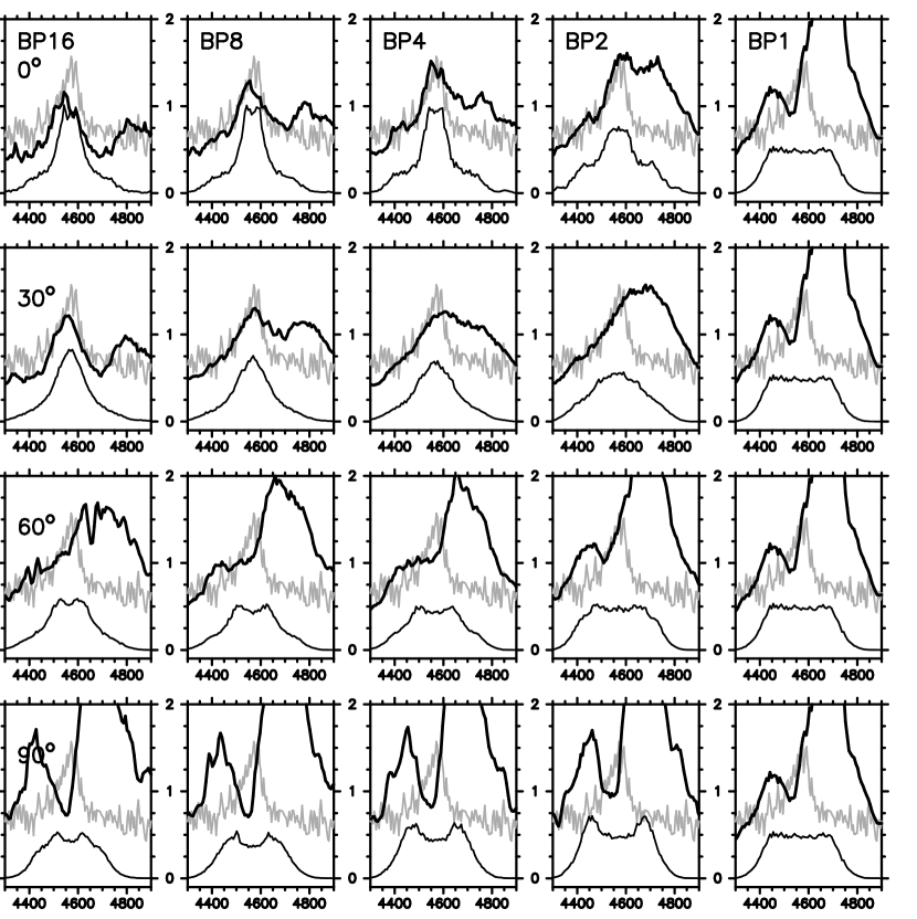
Figure 17: The synthetic spectra of the 2D model around 4600Å (black thick lines) as compared with the observed one of SN 1998bw at 337 days after the B maximum (gray lines). The synthetic spectra are mainly contributed by MgI] 4570Å and forest of [FeII] and [FeIII]. The models are those with $f_{V}=1.6$. See the caption of Fig. 11 for the meanings of each panel. The contribution of MgI] 4570Å is also shown (thin lines).

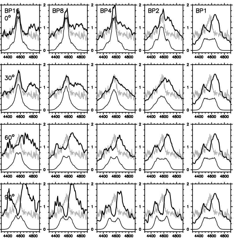
Figure 18: The same with Fig. 17 (MgI] 4570Å and [FeII], [FeIII]), except the model parameter $f_{V}=1.15$.

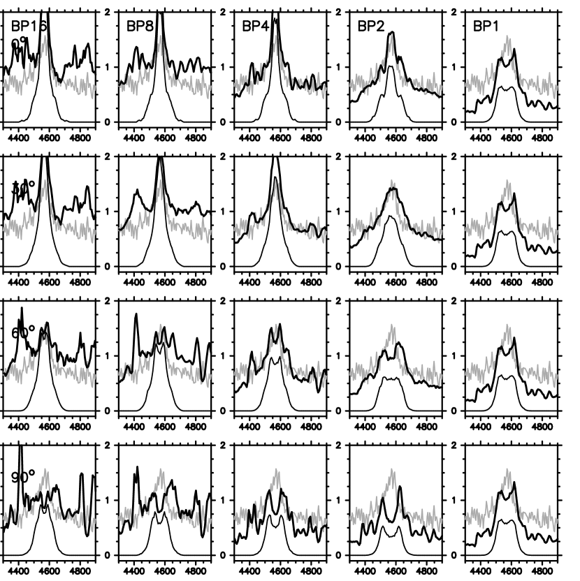
Figure 19: The same with Fig. 17 (MgI] 4570Å and [FeII], [FeIII]), except the model parameter $f_{V}=0.7$.

The observed profile of MgI] 4570Å is sharply peaked, similar to [OI] 6300Å (Patat et al. 2001). The computation of nucleosynthesis in a supernova explosion gives a distribution of Mg similar to that of O. Therefore, the line profile shows characteristics similar to those of O. Figures 17 – 19 show the synthetic line profiles of MgI] 4570Å for various models and viewing angles. The fit to this line is less certain than that of [OI] 6300Å  because of significant contributions of the [FeII] and [FeIII] lines. To examine the characteristics of pure MgI] 4570Å, the contribution of this line is also shown in Figures 17 – 19. The shape of the line favors highly-aspherical models viewed at small $\theta$, supporting the results derived from the [OI] 6300Å profile.

A.4 [CaII] 7291, 7324Å

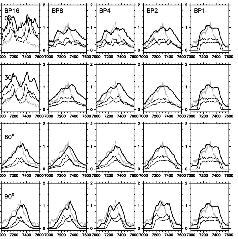
Figure 20: The synthetic spectra of the 2D models around 7300Å (black thick lines) as compared with the observed one of SN 1998bw at 337 days after the B maximum (gray lines). The synthetic spectra are mainly contributed by [CaII] 7291Å, 7324Å, and [FeII] 7155Å, 7172Å, 7388Å, and 7452Å. The models are those with $f_{V}=1.6$. See the caption of Fig. 11 for the meanings of each panel. The contributions of [CaII] 7291Å and 7324Å are also shown (thin lines).

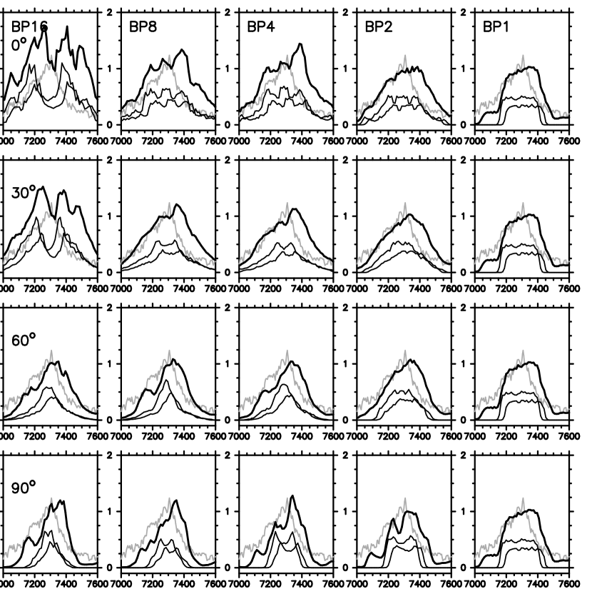
Figure 21: The same with Fig. 20 ([CaII] 7291Å, 7323Å  and [FeII]), except the model parameter $f_{V}=1.15$.

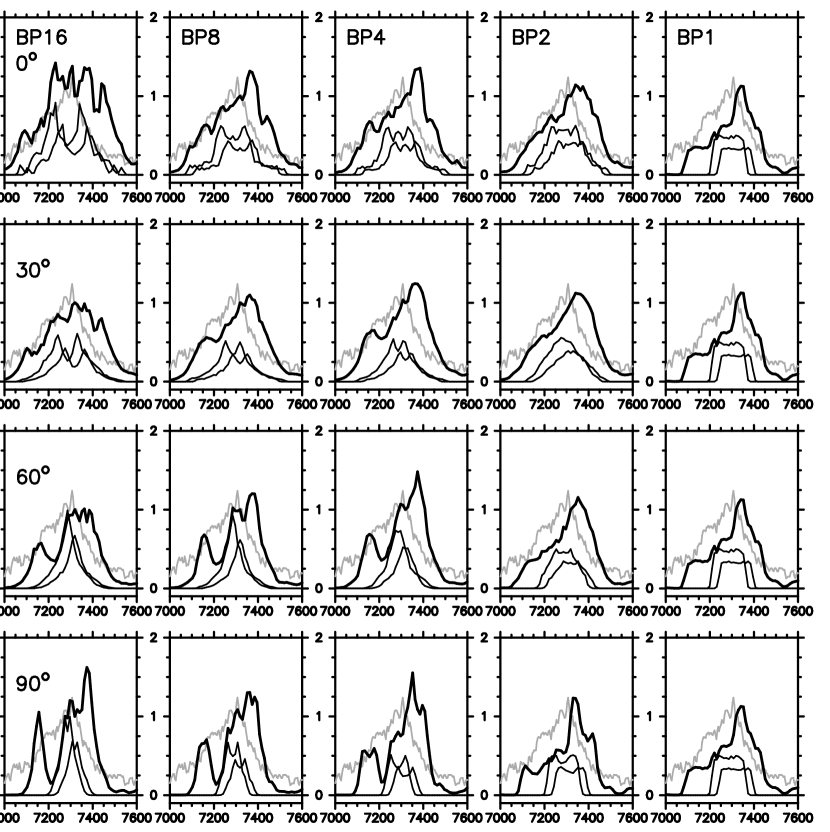
Figure 22: The same with Fig. 20 ([CaII] 7291Å, 7323Å  and [FeII]), except the model parameter $f_{V}=0.7$.

Figures 20 – 22 show synthetic spectra of the present models around 7300Å compared to the observed one at 337 days after the B maximum. The feature is a blend of [CaII] 7291Å, 7324Å, [FeII] 7155Å, 7172Å, 7388Å, and 7452Å, [CoII] 7541Å, and [OII] 7322Å. In a typical nebular condition, the [CaII] lines (whose contributions are individually shown in Figures 20 – 22) probably dominate at the line center, while [FeII] (and [CoII]) fills up the wings. The [OII] 7322Å line is weak in the model, because most oxygen is neutral, as suggested by the strong [OI] 6300Å line.

As shown in the figures, the models are redder than the observations. As mentioned above, the feature is a complex blend making the reason of the failure difficult to identify. For possible origins of the blueshift, see §4.

The [CaII] 7292Å and 7324Å in the models BP16 with small viewing angle ($\theta\sim 0^{\rm o}$) show double peaked profiles because the distribution of Ca, as a product of explosive nucleosynthesis, follows closely that of Fe rather than that of O, which is a product o f hydrostatic burning and a fuel at the explosion (Fig. 5). A higher degree of asphericity (i.e., larger BP) leads to more aspherically distributed Ca. Therefore, the double-peaked profile of Ca for small viewing angle ($\theta\sim 0^{\rm o}$) can be interpreted as two-blobs of Ca moving in opposite directions observed on the symmetry axis. We do not see such a profile in SN 1998bw, suggesting a slightly off-axis viewing angle.

Because of the significant blend of the feature at 7300Å, constraining the energy in the ejecta by fitting this feature is very uncertain. As long as only line width is concerned, less energetic models are preferred if $\theta$ is smaller (e.g., $\theta=0^{\rm o}$), and more energetic ones if $\theta$ is larger (e.g., $\theta=30^{\rm o}$), since narrowing [broadening] the line by smaller [larger] energy must be compensated by broadening [narrowing] the line by smaller [larger] $\theta$.

Table 1: Models

Model	Asphericity (BP)	$f_{V}$	${E_{\rm K}}/10^{51}$ ergs	$M$(56Ni)$/M_{\odot}$	$M_{\rm O}/M_{\odot}$
BP16	16	1.9	33.1	0.79	7.6
	16	1.75	26.5	0.67	7.0
	16	1.6	20.7	0.63	6.4
	16	1.45	15.9	0.60	5.8
	16	1.3	11.5	0.52	5.0
	16	1.15	8.2	0.45	4.4
	16	1.0	5.9	0.34	4.1
	16	0.85	3.8	0.27	3.3
	16	0.7	2.3	0.20	2.8
BP8	8	1.9	34.5	0.75	8.7
	8	1.75	27.5	0.68	8.1
	8	1.6	21.3	0.63	7.3
	8	1.45	15.3	0.55	6.1
	8	1.3	11.5	0.48	5.6
	8	1.15	8.4	0.37	5.1
	8	1.0	5.9	0.32	4.6
	8	0.85	4.0	0.25	4.1
	8	0.7	2.0	0.22	2.6
BP4	4	1.9	32.5	0.63	7.9
	4	1.75	25.9	0.58	7.3
	4	1.6	20.2	0.53	6.7
	4	1.45	15.3	0.45	6.0
	4	1.3	11.2	0.42	5.3
	4	1.15	7.9	0.36	4.5
	4	1.0	5.7	0.30	4.2
	4	0.85	3.7	0.25	3.5
	4	0.7	2.1	0.19	2.6
BP2	2	1.9	36.9	0.55	9.7
	2	1.75	28.9	0.51	8.7
	2	1.6	22.1	0.47	7.8
	2	1.45	16.3	0.43	6.7
	2	1.3	12.2	0.36	6.1
	2	1.15	8.8	0.33	5.5
	2	1.0	6.2	0.27	4.9
	2	0.85	4.1	0.24	4.3
	2	0.7	2.9	0.22	3.4
BP1	1	1.9	37.5	0.54	9.5
	1	1.75	29.7	0.49	8.6
	1	1.6	23.1	0.47	7.7
	1	1.45	16.7	0.43	6.4
	1	1.3	12.7	0.41	5.8
	1	1.15	9.5	0.39	5.4
	1	1.0	6.6	0.33	4.7
	1	0.85	4.1	0.30	3.5
	1	0.7	2.5	0.22	2.9

Figure 2: Synthetic spectra for the modified CO138E30 model. See the caption of Fig. 1. The mass of ⁵⁶Ni is $0.61M_{\odot}$.

Figure 3: Density distribution at 1 day after the explosion. The original CO138E30 (gray) and the modified model (black) are shown. High velocity materials at $>30,000$ km s^-1 are not included in the present study, since they contribute virtually nothing on late phase emission.

Figure 4: Mass fractions of some selected elements and ⁵⁶Ni in the velocity space for (a) the original CO138E30 and for (b) the modified model.

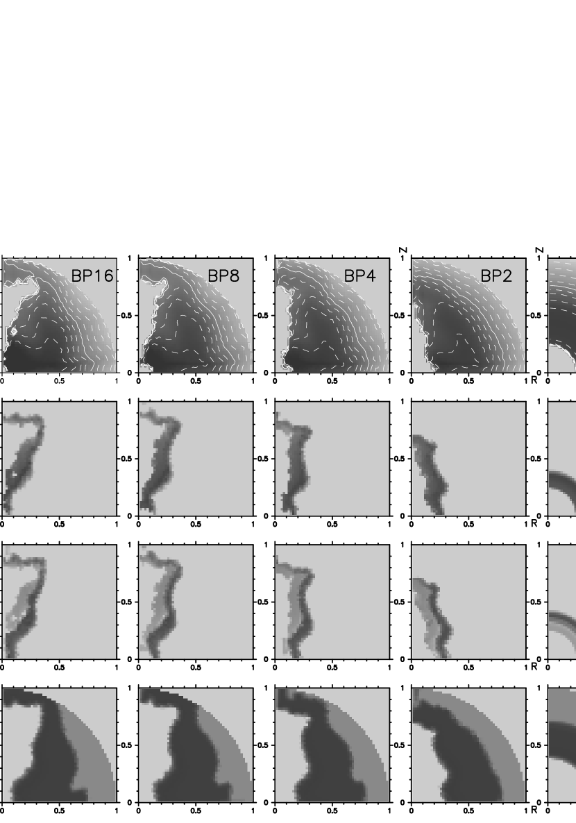
Figure 5: Structure of the ejecta for Models BP16, BP8, BP4, BP2, and BP1 (from left to right) in the ejecta velocity space at a reference time (at 100 seconds). The parameter $f_{V}$ = 1. The axes are $r$ and $z$ components of velocities scaled at $15,000$ km s^-1. For each model, shown here are density, mass fraction of ⁵⁶Ni, Ca, and O (from top to bottom).

Figure 7: Acceptable models for 1998bw. (a) $\theta=0^{\rm o}$ and (b) $\theta=30^{\rm o}$. The figure is obtained by comparing model spectra with the observed one of SN 1998bw at 337 days after the B maximum. The regions surrounded by solid, dashed, and dotted lines contain models which give an acceptable fit to the line profiles around 5200Å ([FeII]), 6300Å ([OI]), and 7300Å ([CaII]), respectively. See §3.4 for details.

Figure 8: Temporal evolution of the synthetic spectra for 2D models as compared with the spectra of SN 1998bw. Shown here are Model BP8 with $f_{V}$=1.15 (a) and $f_{V}$=1.6 (b). The orientation is $\theta=30^{\rm o}$. For presentation, both the synthetic and the observed spectra are multiplied by an arbitrary constant (const₁) and then vertically shifted upward by another factor (const₂). The amounts (const₁, const₂ in units of $10^{-16}$ erg s^-1 cm^-2 Å^-1) are as follows: +125^d (0.1, 1.8), +200^d (0.1, 1.2), +337^d (0.5, 0.6), and +376^d (1.0, 0.0).

Figure 9: Sequence of the spectra of the ”modified” two-dimensional models (black solid lines). Shown here are Model BP8 with $f_{V}$=1.15 (a) and $f_{V}$=1.6 (b). The orientation is $\theta=30^{\rm o}$. The spectra of SN 1998bw (gray lines) and the modified ”one dimensional” CO138E30 model (black dotted line) are also shown. See also the caption of Figure 8. The mass of ⁵⁶Ni in the modified models is $0.40M_{\odot}$ for $f_{V}$=1.15 (a) and $0.56M_{\odot}$ for $f_{V}$=1.6 (b), respectively.

Figure 10: The bolometric light curve of SN 1998bw (gray points; Patat et al. 2001) are compared with the synthetic curve from the 1D original CO138E30 (thin lines) and that from the 2D BP8 model with $f_{V}$=1.15 (thick solid). The mass of ⁵⁶Ni in the 2D model is $0.37M_{\odot}$ (Table 1). In the 1D model, the mass of ⁵⁶Ni is varied to illustrate the difference with the 2D model. $M$(⁵⁶Ni) is $0.64M_{\odot}$ (thin solid) and $0.41M_{\odot}$ (thin dotted) for the 1D model.

References

- axelrod (1980) Axelrod, T.S. 1980, Ph. D. Thesis, University of California at Santa Cruz
- bloom (2003) Bloom, J.S., Frail, D.A., & Kurkarni, S.R. 2003, ApJ, 594, 674
- brown (2000) Brown, G.E., Lee, C.-H., Wijers, R.A.M.J., Lee, H.K., Israelian, G., Bethe, H.A. 2000, New Astronomy, 5, 191
- cappellaro (1997) Cappellaro, E., Mazzali, P.A., Benetti, S., Danziger, I.J., Turatto, M., della Valle, M., Patat, F. 1997, A&A, 328, 203
- chugai (2000) Chugai, N.N. 2000, Astronomy Letters, 26, 797
- clocchiatti (1997) Clocchiatti, A., & Wheeler, J.C. 1997, ApJ, 491, 375
- Della Valle et al. (2003) Della Valle, M., et al. 2003, A&A, 406, L33
- dotani (1987) Dotani, T., et al. 1987, Nature, 330, 230
- foley (2003) Foley, R.J., et al. 2003, PASP, 115, 1220
- frail (2001) Frail, D.A., et al. 2001, ApJ, 562, L55
- Galama et al. (1998) Galama, T. J., et al. 1998, Nature, 395, 670
- heise (2001) Heise, J., in’t Zand, J., Kippen, R.M., Woods, P.M. 2001, in Gamma-Ray Burst in the Afterglow Era, eds. E. Costa, F. Frontera, J. Hjorth (Berlin Heidelberg: Springer), 16
- Hjorth et al. (2003) Hjorth, J., et al. 2003, Nature, 423, 847
- hoeflich (1999) Höflich, P., Wheeler, J.C., Wang, L. 1999, ApJ, 521, 179
- hoeflich (2004) Höflich, P., et al. 2004, ApJ, 617, 1258
- houck (1996) Houck, J.C., & Fransson, C. 1996, ApJ, 456, 811
- Iwamoto et al. (1998) Iwamoto, K., et al. 1998, Nature, 395, 672
- Iwamoto (05) Iwamoto, N., Umeda, H., Tominaga, N., Nomoto, K., Maeda, K. 2005, Science, in press (astro-ph/0505524)
- kawabata (2002) Kawabata, K.S., et al. 2002, ApJ, 580, L39
- Kawabata et al. (2003) Kawabata, K.S., et al. 2003, ApJ, 593, L19
- Kawabata (2004) Kawabata, K., Maeda, K., Deng, J., Nomoto, K., Mazzali, P.A., Pian, E., Wang, L. Ohyama, Y., Iye, M. 2004, IAUC, 8410
- kif (2000) Kifonidis, K., Plewa, T., Janka-H.-Th., Müller, E. 2000, ApJ, 531, L123
- (23) Kozma, C., & Fransson, C. 1998a, ApJ, 496, 946
- (24) Kozma, C., & Fransson, C. 1998b, ApJ, 497, 431
- kozma (2005) Kozma, C., et al. 2005, A&A, 437, 983
- leonard (2002) Leonard, D.C., Filippenko, A.V., Chornock, R., & Foley, R.J. 2002, PASP, 114, 1333
- MacFadyen & Woosley (1999) MacFadyen, A. I., & Woosley, S. E. 1999, ApJ, 524, 262
- maeda (2002) Maeda, K., Nakamura, T., Nomoto, K., Mazzali, P.A., Patat, F., Hachisu, I. 2002, ApJ, 565, 405
- (29) Maeda, K., Mazzali, P.A., Deng, J., Nomoto, K., Yoshii, Y., Tomita, H., Kobayashi, Y. 2003a, ApJ, 593, 931
- (30) Maeda, K., & Nomoto, K. 2003b, ApJ, 598, 1163
- malesani (2004) Malesani, D., et al. 2004, ApJ, 609, L5
- mat (2001) Matheson, T., Filippenko, A.V., Li, W., Leonard, D.C. 2001, ApJ, 121, 1648
- Matheson et al. (2003a) Matheson, T., et al. 2003, ApJ, 599, 394
- (34) Matheson, T. 2004, in the proceedings of ”Supernovae as Cosmological Lighthouses” (Padua: ASP), ASP conf. series, in press (astro-ph/0410668)
- matz (1988) Matz, S.M., et al. 1988, Nature, 331, 416
- Mazzali, Iwamoto, & Nomoto (2000) Mazzali, P.A., Iwamoto, K., & Nomoto, K. 2000, ApJ, 545, 407
- mazzali (2001) Mazzali, P.A., Nomoto, K., Patat, F., Maeda, K. 2001, ApJ, 559, 1047
- mazzali (2005) Mazzali, P.A., Kawabata, K.S., Maeda, K., et al. 2005, Science, 308, 1284
- mckenzie (1999) McKenzie, E.H., & Schaefer, B.E. 1999, PASP, 111, 964
- milne (2001) Milne, P.A., The, L.-S., Leising, M.D. 2001, ApJ, 559, 1019
- nagataki (1998) Nagataki, S., Shimizu, T.M., Sato, K. 1998, ApJ, 495, 413
- nakamura (1998) Nakamura, T. 1998, Prog. Theor. Phys. 100, 921
- Nakamura et al. (2001) Nakamura, T., Mazzali, P. A., Nomoto, K., Iwamoto, K. 2001, ApJ, 550, 991
- Nomoto et al. (2003) Nomoto, K., Maeda, K, Mazzali, P. A., Umeda, H., Deng, J., & Iwamoto, K. 2004, in Stellar Collapse, ed. C. L. Fryer (Kluwer: Dordrecht), 277 (astro-ph/0308136)
- paczynski (1998) Paczynski, B. 1998, ApJ, 494, L45
- (46) Patat, F., et al. 2001, ApJ, 555, 900
- (47) Piran, T. 1999, Phys. Rept. 314, 575
- (48) Ruiz-Lapuente, P., & Lucy, L.B. 1992, ApJ, 400, 127
- sollerman (2000) Sollerman, J., Kozma, C., Fransson, C., Leibundgut, B., Lundqvist, P., Ryde, F., Woudt, P. 2000, ApJ, 537, L127
- sollerman (2004) Sollerman, J., et al. 2004, A&A, 428, 555
- Stanek et al. (2003) Stanek, K. Z., et al. 2003, ApJ, 591, L17
- sunyaev (1987) Sunyaev, R., et al. 1987, Nature, 330, 227
- thomsen (2004) Thomsen, B., et al. 2004, A&A, 419, L21
- wang (2003) Wang, L., Baade, D., Höflich, P., & Wheeler, J.C. 2003, ApJ, 592, 457
- wheeler (2000) Wheeler, J.C., Yi, I., P., Wang, L. 2000, ApJ, 537, 810
- (56) Woosley, S.E. 1993, ApJ, 405, 273
- woosley (1999) Woosley, S.E., Eastman, E.G., & Schmidt, B.P. 1999, ApJ, 516, 788
- yamazali (2003) Yamazaki, R., Yonetoku, D., & Nakamura, T. 2003, ApJ, 594, L79
- yoshii (2003) Yoshii, Y., et al. 2003, ApJ, 592, 467