X-Ray Emission by A Shocked Fast Wind from the Central Stars of Planetary Nebulae

Abstract

We calculate the X-ray emission from the shocked fast wind blown by the central stars of planetary nebulae (PNs) and compare with observations. Using spherically symmetric self similar solutions, we calculate the flow structure and X-ray temperature for a fast wind slamming into a previously ejected slow wind. We find that the observed X-ray emission of six PNs can be accounted for by shocked wind segments that were expelled during the early PN phase, if the fast wind speed is moderate, $v_{2}\sim$ 400-600 $~{}\rm{km}~{}{\rm s}^{-1}$, and the mass loss rate is a few times $10^{-7}M_{\odot}~{}\rm{yr}^{-1}$. We find, as proposed previously, that the morphology of the X-ray emission is in the form of a narrow ring inner to the optical bright part of the nebula. The bipolar X-ray morphology of several observed PNs, which indicates an important role of jets rather than a spherical fast wind, cannot be explained by the flow studied here.

Subject headings: Subject headings: stars: mass loss stars: winds, outflows planetary nebulae: X-ray X-rays: ISM

1 INTRODUCTION

The sample of well observed planetary nebulae (PNs) with extended spatially resolved X-ray structures is large enough to start answering open questions on the shaping of and the emission from PNe. This sample includes PNs observed by the Chandra X-ray Observatory (CXO): BD +30^∘3639 (Kastner et al. 2000; Arnaud et al. 1996 detected X-rays in this PN with ASCA), NGC 7027, (Kastner, et al. 2001), NGC 6543 (Chu et al. 2001), Henize 3-1475 (Sahai et al. 2003), Menzel 3 (Kastner et al. 2003), as well as PNs observed with XMM-Newton: NGC 7009 (Guerrero et al. 2002), NGC 2392 (Guerrero et al. 2005), and MGC 7026 (Gruendl et al. 2004). For some other PNs no X-ray emission has been detected: M1-16 (Soker & Kastner 2003), NGC 7293 (Guerrero et al. 2001), Hen 2-99 (Kastner et al. 2005), and NGC 2346 (Gruendl et al. 2004). It should be pointed out that X-ray emission is expected from all PNs, but many PNs emit X-rays below the current detection limit. In NGC 40, only a careful analysis, looking selectively at photons in a specific energy band, has yielded a positive detection (Kastner et al. 2005). The main question now as formulated by Soker & Kastner (2003) is: What is the (astro)physical origin of the hot gas in the extended X-ray emission region. There are several plausible answers. The X-ray emitting gas may result from shocked fast wind segments that were expelled by the central star during the early PN phase or late post-asymptotic giant branch (AGB) phase, when the wind speed was moderate, $\sim 500~{}\rm{km}~{}\rm{s}^{-1}$. Alternatively, the X-ray emitting gas may result from a collimated fast wind (CFW; or jets if the wind is well collimated) blown in conjunction with the companion to the central star during the late AGB phase or early post-AGB phase. Soker & Kastner (2003) conclude that in order to account for the observed X-ray temperature and luminosity, both the evolution of the wind from the central star and the adiabatic cooling of the post-shocked wind’s material must be considered.

Extended X-ray emission in PNs was expected based on the presence of a fast wind driven by the central star during the late post-AGB phase and early PN phase, as the interaction between this fast wind and slower-moving material, ejected when the central star was still an AGB star, should lead to energetic shocks. The same wind-wind interaction plays some role in shaping many PNs (e.g., Balick & Frank 2002, and references therein). However, CFWs (or jets) must play a more significant role in the shaping of many PNs (but not all PNs) than the spherical fast wind from the central star plays (Soker 2004). Hence, the processes behind the extended X-ray emission are tied to the shaping processes of PNs (Kastner et al. 2003), although not all shaping processes will lead to X-ray emission. X-ray-emitting regions of some PNs are quite asymmetric. This asymmetry results in large part from extinction (Kastner et al. 2003). However, extinction by itself cannot account for all of the observed X-ray asymmetries and structural irregularities, and other processes should be considered (Kastner et al. 2003).

These findings, though, are not enough by themselves to reveal the origin of the X-ray emitting gas, whether it is from a CFW blown by a companion during the AGB and/or early post-AGB phase, or whether the spherical fast wind blown by the central star during the late post-AGB phase is the source of the X-ray emitting gas. Theoretical calculations of the X-rays expected in these two cases, and quantitative comparison with observations are required for that purpose. It is very likely that both processes contribute to a certain degree in different PNs. In the present paper we study the expected contribution from the fast spherical wind blown by the central star. We use the self-similar solution of Chevalier & Imamura (1983; hereafter CI83) and estimate the conditions under which the wind blown by the central star can explain the observed X-ray properties of PNs. In Section 2, we present the theoretical method based on the self similar solution as well as the physical parameters used to determine the X-ray emission. The results of the calculations and the comparison with observations are discussed in Sections 3 and 4, respectively. A summary of our main findings is given in Section 5.

2 THEORETICAL METHOD

2.1 Self Similar Solution

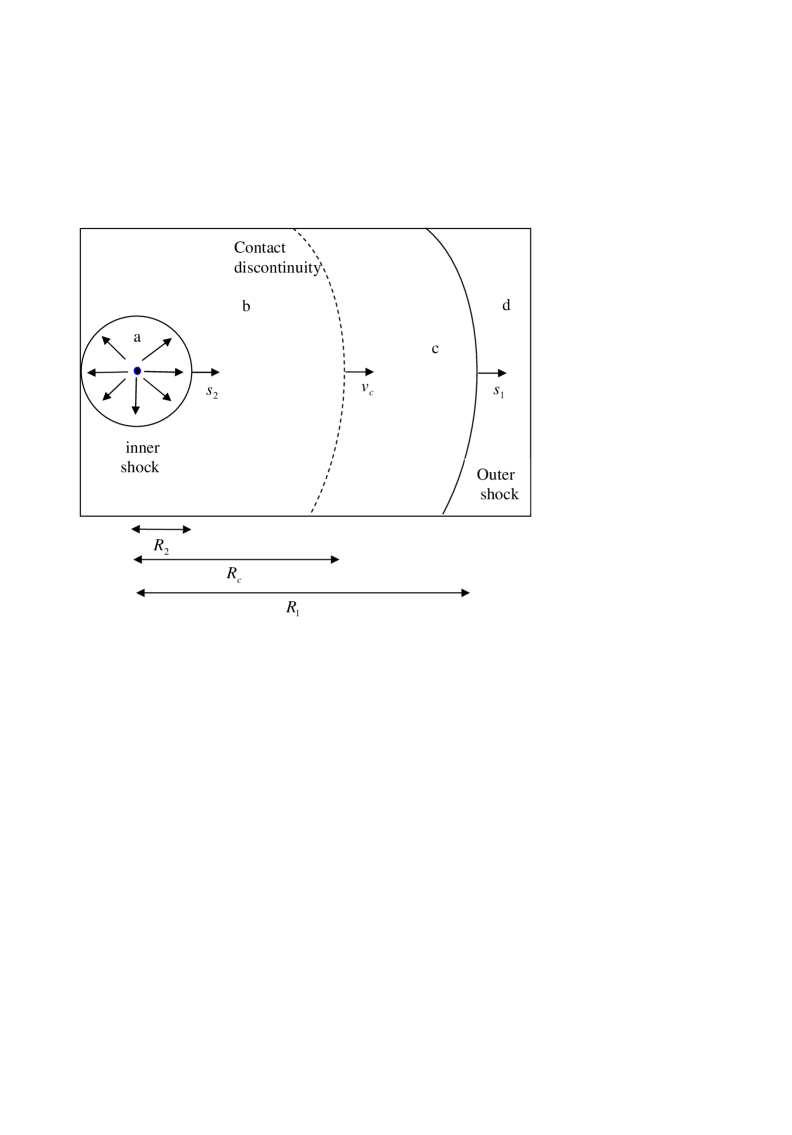
Figure 1: A schematic drawing of the interacting stellar wind flow structure. The regions indicated are: (a) the undisturbed central star fast wind; (b) the hot bubble formed by the shocked central star fast wind; (c) the shocked slow wind; and (d) the nebular gas (the pre-shock AGB wind). $s_{1}$ and $s_{2}$ represent the forward and reverse shocks velocities.

CI83 present a self-similar solution to the following flow structure. A spherically symmetric slow wind with a constant mass loss rate $\dot{M}_{1}$ and a constant velocity $v_{1}$ fills the space around the center $r=0$ where the star resides(see Fig. 1). At time $t=0$ the slow wind ceases and a spherically symmetric fast wind of mass loss rate $\dot{M}_{2}$ and a constant velocity $v_{2}$ expands and collides with the slow wind. The slow and fast wind do not mix, but rather are separated by an evolving spherical surface termed the contact discontinuity corresponding to a radius $R_{c}(t)$ (see Fig. 2 by Volk & Kwok 1985 and fig. 1 here). A spherical shock wave runs outwards into the slow wind at radius $R_{1}(t)>R_{c}(t)$. At the same time, a spherical inward (reverse) shock wave propagates through the fast wind down to radius $R_{2}$, thus heating the region $R_{2}<r<R_{c}$. This region is termed the hot bubble. In the self similar solution, there are no imposed characteristic length scales or time scales, hence the evolution with time and distance depends only on the ratio $r/t$.

We are interested in the contribution of the shocked spherically symmetric fast wind blown by the central star during the late post-AGB and early PN phases to the X-ray emission. Therefore, we examine only the region inward to the contact discontinuity $R_{2}<r<R_{c}$. The solution in that region is given by specifying two dimensionless parameters (CI83): (1) the ratio $b_{2}=v_{2}/s_{2}$, where $s_{2}=\dot{R}_{2}(t)$ is the reverse shock speed; and (2) the Mach number, which is the ratio $M_{2}=(v_{2}-s_{2})/c_{2}$, where $c_{2}$ is the sound speed in the pre-shock fast wind gas. For the appropriate parameters in the present case of $v_{2}\geq 300~{}\rm{km}~{}\rm{s}^{-1}$ and central star effective temperature of $\sim 30,000~{}\rm{K}$, $v_{2}>>c_{2}$ and the Mach number of the fast wind is very large, practically infinite in the self-similar regime. For large Mach numbers the value of $b_{2}$ is determined by the two ratios $v_{1}/v_{2}$ and $\dot{M}_{1}/\dot{M}_{2}$ (Fig. 6. of CI83).

For large Mach numbers pressure equilibration is efficient and thus the pressure is fairly constant throughout the hot bubble (Fig. 4 of CI83 and Figs. 2 and 3 below). By assuming constant pressure inside the hot bubble, Volk & Kwok (1985) were able to solved for a time delay $\tau_{0}>0$ between the end of the slow wind and the beginning of the fast wind. Because the wind is continuous and there is no real delay between the slow and fast winds, we prefer to use the self similar solution to determine the exact pressure profile inside the hot bubble. For the present study, it is adequate to use the contact discontinuity speed as given by Volk & Kwok (1985; their Eq. 4):

$$\left(\frac{v_{c}}{v_{1}}\right)^{3}-2\left(\frac{v_{c}}{v_{1}}\right)^{2}+\left(\frac{v_{c}}{v_{1}}\right)=\frac{1}{3}\frac{\dot{M}_{2}v_{2}^{2}}{\dot{M}_{1}v_{1}^{2}}.$$ (1)

For the radius of the contact discontinuity we use the approximation $R_{c}=v_{c}t$, where $t$ is the age of the fast wind assumed to be also the age of the nebula. This time enters as an additional parameter into our model. It is easy to find the location of the reverse shock by equating the pressure in the hot bubble given by Volk & Kwok (1985) to the pre-shock ram pressure of the fast wind. This gives for $R_{2}$:

$$\eta\equiv\frac{R_{2}}{R_{c}}=\left(\frac{\dot{M}_{2}v_{2}}{\dot{M}_{1}v_{1}}\right)^{1/2}\frac{v_{1}}{v_{c}-v_{1}}$$ (2)

In summary, our calculations require the parameters $\dot{M}_{1}$, $\dot{M}_{2}$, $v_{1}$, $v_{2}$, and $t$ as input. The self similar solution then provides the density and temperature (and pressure) profiles from $R_{2}$ to $R_{c}$. In the present study, we mainly vary $v_{2}$ and $\dot{M}_{2}$, on which the X-ray properties are strongly dependent with $v_{1}=10~{}\rm{km}~{}\rm{s}^{-1}$ kept constant for all cases.

2.2 Radiative Cooling

The shocked fast wind loses energy and cools down as it emits X-ray and UV radiation. This cooling must be considered in a full numerical study as it cannot be dealt with in the self similar formalism. In the present study, we do include cooling, but in a rather crude way. We remove from the calculation of the X-ray luminosity gas shells whose radiative cooling times are shorter than the age of the nebula $t$.

The cooling (energy loss) rate per unit volume per unit time is $\Lambda n_{e}n_{p}$, where $n_{e}$ and $n_{p}$ are the electron and proton number densities, respectively. In the temperature range $2\times 10^{5}$ K $\lesssim$ T $\lesssim 2\times 10^{7}$ K, the cooling function $\Lambda$ is approximately 10${}^{-22}(T/10^{6}\mathrm{K})^{-1/2}~{}\rm{erg}~{}\rm{cm}^{3}~{}\rm{s}^{-1}$, which is an approximation to Fig. 6 of Gaetz et al. (1988). As the gas cools its cooling time decreases quickly. Soker & Kastner (2003) take this into account, and write for the cooling time

$$\tau_{\rm cool}\simeq k_{\rm cool}\frac{nkT}{\Lambda n_{e}n_{p}}=k_{\rm cool}\frac{P}{\Lambda n_{e}n_{p}},$$ (3)

where $n$ is the total number density including protons, electrons and all other atoms and ions. At constant pressure and slow variation with temperature of $T/\Lambda$, $k_{\rm cool}\simeq 5/2$. However, here $T/\Lambda\propto T^{3/2}$, and the cooling time is somewhat shorter. Soker & Kastner (2003) included also adiabatic cooling in $k_{\rm cool}$, and for their crude estimate took $k_{\rm cool}=1$. As adiabatic cooling is already included in the self-similar solution, we take $k_{\rm cool}=5/2$. Substituting for the typical values, Soker & Kastner (2003) find

$$\tau_{\rm cool}\simeq 400\left(\frac{T}{10^{6}~{}\rm{K}}\right)^{5/2}\left(\frac{v_{\rm c}}{20~{}\rm{km}~{}\rm{s}^{-1}}\right)^{2}\left(\frac{t}{500~{}\rm{yr}}\right)^{2}\left(\frac{\dot{M}_{2}v_{2}}{3\times 10^{-5}M_{\odot}~{}\rm{yr}^{-1}~{}\rm{km}~{}\rm{s}^{-1}}\right)^{-1}\left(\frac{\eta}{0.3}\right)^{2}~{}\rm{yr}.$$ (4)

For a parcel of gas to stay in the X-ray emitting temperature for a time $t$ the cooling time must be $\tau_{\rm cool}\gtrsim t$, which for the scaling used in equation (4) is equivalent to

$$T_{\rm min}\gtrsim 10^{6}\left(\frac{v_{\rm c}}{20~{}\rm{km}~{}\rm{s}^{-1}}\right)^{-0.8}\left(\frac{t}{500~{}\rm{yr}}\right)^{-0.4}\left(\frac{\dot{M}_{2}v_{2}}{3\times 10^{-5}M_{\odot}~{}\rm{yr}^{-1}~{}\rm{km}~{}\rm{s}^{-1}}\right)^{0.4}\left(\frac{\eta}{0.3}\right)^{-0.8}.$$ (5)

Soker & Kastner (2003) estimate the total X-ray luminosity of the shocked fast wind as

$$L_{x}\simeq 10^{33}\left(\frac{T}{10^{6}~{}\rm{K}}\right)^{-2}\left(\frac{v_{\rm c}}{20~{}\rm{km}~{}\rm{s}^{-1}}\right)^{-2}\left(\frac{t}{500~{}\rm{yr}}\right)^{-2}\left(\frac{\Delta t}{100~{}\rm{yr}}\right)$$ (6)

$$\left(\frac{\dot{M}_{2}v_{2}}{3\times 10^{-5}M_{\odot}~{}\rm{yr}^{-1}~{}\rm{km}~{}\rm{s}^{-1}}\right)^{2}\left(\frac{\eta}{0.3}\right)^{-2}~{}\rm{erg}~{}\rm{s}^{-1},$$

where $\Delta t$ is the time during which the central star blows the fast wind segment at a speed of $v_{2}$ which is responsible for most of the X-ray emission.

In the present work, we use the cooling function $\Lambda$ for solar abundances from Sutherland & Dopita (1993; their table 6), linearly interpolating their data to obtain a continuous function $\Lambda(T)$. Rapidly cooling regions having $\tau_{\rm cool}<t$ are not included in the computation of the X-ray emission. It is important to note that this is not a fully self-consistent treatment, because ($i$) we do not follow the evolution of gas parcels with radiative cooling, but rather examine the radiative cooling time at a specific time, ($ii$) we do not take into account the process by which ambient gas from hotter regions of the bubble fills in for the gas that has cooled to $T\ll 10^{6}~{}\rm{K}$, compressed, and now occupies only a small volume of the flow. However, in the relevant self similar solutions studied here, we find that only small regions of the flow are associated with short cooling times $\tau_{\rm cool}<t$. Therefore, the present treatment is in fact appropriate for the present purpose of studying the behavior of the self-similar regime.

2.3 X-Ray Emission

The X-ray luminosity is calculated by integrating the emissivity over the hot bubble .

$$L_{x}(R_{c})=\int_{R_{2}}^{R_{c}}n_{e}n_{p}\Lambda_{0210}(T)4\pi r^{2}dr,$$ (7)

(but ignoring regions with $\tau_{\rm cool}<t$) where $\Lambda_{0210}(T)n_{e}n_{p}$ is the power emitted per unit volume in the energy range $0.2-10~{}\rm{keV}$. This range is chosen to reflect approximately the sensitivity regime of the Chandra and XMM-Newton telescopes and science instruments. The function $\Lambda_{0210}(T)$, which serves here essentially as an X-ray energy emission rate coefficient, is obtained from the APEC data base (Smith et al. 2001) using XSPEC version 11.3.1 (Arnaud 1996).

In most X-ray observations of PNs the spatial resolution is not high, and/or there are not enough photons to obtain a spatially resolved temperature profile. In those cases, the total X-ray spectrum of the PN is fitted with an isothermal model, thus assigning a single, best-fit temperature to the entire hot bubble. For comparison with observations we therefore define an X-ray weighted average temperature for the hot bubble by:

$$T_{x}=\frac{1}{L_{x}}\int_{R_{2}}^{R_{c}}Tn_{e}n_{p}\Lambda_{0210}(T)4\pi r^{2}dr.$$ (8)

or in terms of the more easily observed quantity, the emission measure distribution $EMD(T)$

$$T_{x}=\frac{1}{L_{x}}\int_{R_{2}}^{R_{c}}T\Lambda_{0210}(T)EMD(T)dT.$$ (9)

where $L_{x}$ is taken from Eq. (7) and $EMD(T)$ is defined as:

$$EMD(T)\equiv n_{e}n_{p}\frac{dV}{dT}=n_{e}n_{p}4\pi r^{2}\frac{dr}{dT}$$ (10)

The right hand side of Eq. (10) is valid for the spherically symmetric case. $EMD(T)$ can be calculated from the self similar temperature profile $T(r)$ and the results will be presented in the next section. Note that as for $L_{x}$, in calculating $T_{x}$ cooling is taken into account by the exclusion of fast cooling regions ($\tau_{\rm cool}<t$). In practice, the observed temperature is obtained by fitting spectral models to the X-ray photon (not energy) spectrum using $\chi^{2}$ minimization techniques (Arnaud  1996). To that end, it would have been more rigorous to use the X-ray photon emission rate coefficient instead of $\Lambda_{0210}(T)$. In a sense it would have also been better to take the square of $EMD(T)$ as the distribution function in Eq. (9) instead of simply $EMD(T)$. However, we have checked and found that these corrections have a negligible effect of only a few percent on the calculated result for $T_{x}$ (due to the dominance of the high-density low-temperature regions in the flow). Therefore, for simplicity we have used Eqs. (8) and (9) in the forms given above.

2.4 Outline of Calculations

The set up of the calculations is as follows:

1. The parameters specified are: The time of the observation $t$; The velocities, $v_{1}$ and $v_{2}$ and the mass loss rates $\dot{M}_{1}$ and $\dot{M}_{2}$, of the slow and fast winds, respectively.

2. The contact discontinuity velocity $v_{c}$ is calculated from equation (1).

3. The position (radius) of the contact discontinuity is calculated by $R_{c}=v_{c}t$.

4. The position of the inner (reverse) shock $R_{2}$ (or of $\eta$) is given by equation (2).

5. The density $n(r)$ and temperature $T(r)$ profiles in the hot bubble are found from the self-similar solution of CI83; the self-similar equations are integrated from $R_{2}$ to $R_{c}$, where at $R_{c}$ the gas follows the contact discontinuity, i.e., $v=v_{c}$ ($U=1$ in the terminology of CI83).

6. The radiative cooling time $\tau_{\rm cool}(r)$ is calculated at each radius by equation (3), with $\Lambda(T)$ from Sutherland & Dopita (1993) and using $k_{cool}$ = 5/2 as explained above.

7. If $\tau_{\rm cool}<t$, the gas at that radius is not included in the computation of the X-ray emission.

8. The X-ray luminosity and average temperature are calculated from Eqs. (7) and (8), respectively.

9. The calculations are repeated for different sets of parameters.

3 RESULTS

In order to explore the self similar solutions to our problem we carried out several runs, which are summarized in Table 1. We examine three cases for the slow wind parameters: $\dot{M}_{1}=3\times 10^{-6}M_{\odot}~{}\rm{yr}^{-1}$, $\dot{M}_{1}=7\times 10^{-6}M_{\odot}~{}\rm{yr}^{-1}$, and $\dot{M}_{1}=3\times 10^{-5}M_{\odot}~{}\rm{yr}^{-1}$. For each $\dot{M}_{1}$ value, we take three $v_{2}$ values of 300 $~{}\rm{km}~{}{\rm s}^{-1}$, 500 $~{}\rm{km}~{}{\rm s}^{-1}$, and 700 $~{}\rm{km}~{}{\rm s}^{-1}$. The slow wind velocity $v_{1}$ is assumed to be 10 $~{}\rm{km}~{}{\rm s}^{-1}$ throughout our calculations. For all runs $\dot{M}_{2}$ is chosen so that $\dot{M}_{1}v_{1}=\dot{M}_{2}v_{2}$. For each time $t$, we can calculate the temperature and density profiles.

One property of the solution should be emphasized. The X-ray emitting gas resides close to the contact discontinuity. Faster gas with $v_{2}\gtrsim 700~{}\rm{km}~{}\rm{s}^{-1}$, which was expelled more recently in the evolution, does not contribute to the X-ray luminosity. Therefore, it does not matter whether at later times the mass loss rate and fast wind velocity were constant as assumed here (this is the limitation of the self similar solution), or whether the velocity increases and mass loss decreases as is known to occur in PNs. In either case, the X-ray emission will come from gas residing near the contact discontinuity that was expelled when the PN was young, and even as early as the post-AGB phase when the fast wind speed was $v_{2}\simeq 400-600~{}\rm{km}~{}\rm{s}^{-1}$. It is expected that at later times the observed fast wind will be much faster, as observed in many PNs. In other words, it is not the presently or recently blown wind that is responsible for the X-ray emission. This is why the self-similar solution is adequate for our goal.

Table 1: Cases Calculated

Run	$\dot{M}_{1}$	$\dot{M}_{2}$	$v_{2}$	$v_{c}$	$\eta$	line
	$M_{\odot}~{}\rm{yr}^{-1}$	$M_{\odot}~{}\rm{yr}^{-1}$	$~{}\rm{km}~{}\rm{s}^{-1}$	$~{}\rm{km}~{}\rm{s}^{-1}$
A3	$3\times 10^{-6}$	$1\times 10^{-7}$	$300$	$28.6$	0.52	solid
A5	$3\times 10^{-6}$	$6\times 10^{-8}$	$500$	$32.6$	0.42	dashed
A7	$3\times 10^{-6}$	$4.33\times 10^{-8}$	$700$	$35.6$	0.37	dotted
B3	$7\times 10^{-6}$	$2.33\times 10^{-7}$	$300$	$28.6$	0.52	solid
B4	$7\times 10^{-6}$	$1.75\times 10^{-7}$	$400$	$30.8$	0.44
B5	$7\times 10^{-6}$	$1.40\times 10^{-7}$	$500$	$32.6$	0.42	dashed
B6	$7\times 10^{-6}$	$1.17\times 10^{-7}$	$600$	$34.2$	0.38
B7	$7\times 10^{-6}$	$1\times 10^{-7}$	$700$	$35.6$	0.37	dotted
C3	$3\times 10^{-5}$	$1\times 10^{-6}$	$300$	$28.6$	0.52	solid
C5	$3\times 10^{-5}$	$6\times 10^{-7}$	$500$	$32.6$	0.42	dashed
C7	$3\times 10^{-5}$	$4.28\times 10^{-7}$	$700$	$35.6$	0.37	dotted

Notes: (1) For all runs $v_{1}=10~{}\rm{km}~{}\rm{s}^{-1}$ (2) $\eta\equiv R_{2}/R_{c}$. (3) Runs B4 and B6 are just shown in Fig. 6

3.1 General Characteristics

The self similar solutions all have qualitatively similar profiles, a good example of which are those shown in Fig. 2 and 3. In Fig. 2 we have chosen $R_{c}=3\times 10^{16}~{}\rm{cm}$ which corresponds to $t=291~{}\rm{yr}$ for Run B5. It can be seen that from the inner radius $R_{2}$, the density rises outwards, first gradually, but then sharply peaking (tending to infinity) as the fast wind accumulates towards the contact discontinuity $R_{c}$. On the other hand, the temperature is high around the inner radius (where the density is low) and decreases to very low temperatures, much below X-ray temperatures, towards $R_{c}$, which is expected at these high densities at the infinite Mach number limit. Indeed, as seen from Fig. 2, the pressure profile does not change significantly within the hot bubble. The earlier a gas segment is shocked, the closer it is to the present-day contact discontinuity. Gas segments which were shocked early suffer large volume expansion as the bubble grows, hence strong adiabatic cooling. The mass profile (integral of mass density over volume) is also plotted in Fig. 2. We have used this mass profile to verify mass conservation in our calculations in the sense of:

$$\int_{R_{2}}^{R_{c}}\mu m_{p}n4\pi r^{2}dr=\dot{M}_{2}t$$ (11)

where $\mu m_{p}$ is the average particle mass.

3.2 Cooling Effect and X-Ray Emission

The high-density outer region of the hot bubble can cool relatively quickly. In particular, the cooling time can be shorter than the age of the flow. Obviously, this effect becomes increasingly important as the density increases with $\dot{M}_{2}$. Fig. 3 presents the results for Run C5, again for $R_{c}=3\times 10^{16}~{}\rm{cm}$, which corresponds here to an age of $t$ = 291  yr. In this run, $\dot{M}_{2}=6\times 10^{-7}M_{\odot}~{}\rm{yr}^{-1}$, which is about four times larger than $\dot{M}_{2}$ in Run B5. This is reflected in the four-times higher density values seen in Fig. 3 compared with those of Fig. 2. The high density results in shorter cooling times for Run C5. Consequently, larger regions of the hot bubble near the contact discontinuity need to be disregarded when calculating the X-ray emission.

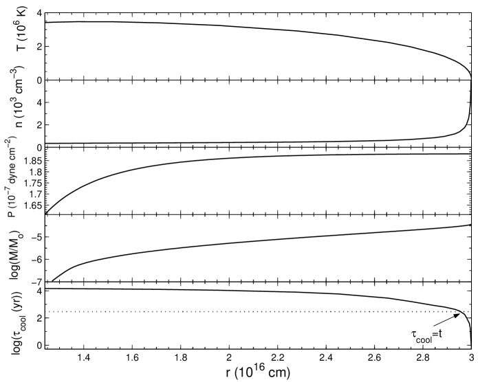
Figure 2: The gas temperature, total number density, pressure, the total gas mass $M(r)$ (logarithmic scale in units of $M_{\odot}$), and cooling time (logarithmic scale in years), between $R_{2}$ and $R_{c}$ as a function of the radius $r$, for Run B5 at an age of 291 yr. The dotted line in the third panel mark the age of the flow (the time since the beginning of the fast wind).

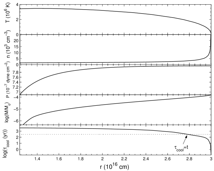
Figure 3: The same as Fig. 2 but for Run C5. The radius where cooling time equals the age, is smaller than in the lower density runs in Fig. 2. Note the different scales compared with Fig. 2.

In order to elucidate on the effect of the removal of the cool gas on the total X-ray luminosity $L_{x}$ in the $0.2-10~{}\rm{keV}$ band, we have plotted in Fig. 4 the total X-ray luminosity as a function of time $t$, once taking radiative cooling into account (by disregarding regions that have cooled- thick lines in Fig. 4), and also when cooling is neglected (thin lines). The three cases considered in Fig. 4, namely Runs B3, B5, and B7, are all for $\dot{M}_{1}=7\times 10^{-6}M_{\odot}~{}\rm{yr}^{-1}$, but for different fast-wind velocities. As can be expected, in the slower wind case (Run B3), the temperature is lowest and $\dot{M}_{2}$ is highest, therefore the density is highest and the cooling time is shortest. It can be seen that the effect of cooling is, indeed, most significant for this case, whereas for higher velocities, the cooling effect is essentially unimportant.

Fig. 4 also demonstrates that the X-ray luminosity $L_{x}$ is highest for a fast wind velocity $v_{2}$ = 500 $~{}\rm{km}~{}{\rm s}^{-1}$, i.e., Run B5. Both lower and higher velocities result in less X-ray emission than in this case (B5). The lower luminosity for $v_{2}$ = 300 $~{}\rm{km}~{}{\rm s}^{-1}$ (B3) is due to the fact that the shocked gas is colder than typical X-ray temperatures and a large fraction of the radiation is emitted below $0.2~{}~{}\rm{keV}$, which is our chosen lower limit for $L_{x}$. The reason for the lower luminosity in the case of $v_{2}$ = 700 $~{}\rm{km}~{}{\rm s}^{-1}$ (B7) is different. In this case, the temperature is high and $\dot{M}_{2}$ is low, therefore the density is low.

In Fig. 4, we also plot $L_{x}$ as given by equation (6). That equation is derived under different assumptions than the ones used in the self similar analysis. In order to make the comparison meaningful, we take $\Delta t=t/5$ as in Soker & Kastner (2003), and the bubble temperature is taken to be the post-shock temperature for Run B5, $T=3.5\times 10^{6}$ K. The $t^{-1}$ dependence is roughly the same and the difference in X-ray luminosity is relatively small between that found in run B5 and that given by equation (6), considering the different assumptions entering the two methods (Soker & Kastner 2003).

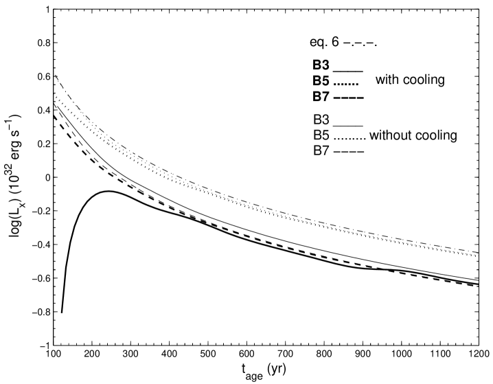
Figure 4: The luminosity as a function of the wind age $t={R_{c}}/{v_{c}}$, for Runs B3 (solid lines) B5 ( dotted lines) and B7 (dashed lines). Thick lines give the luminosity when gas parcels with cooling time shorter than the bubble’s age are not considered; this will be the cases presented for the rest of the paper. For comparison thin lines present the same run but when cooling is not taken into account, and the X-ray contribution of cold parcels of gas is included. The dashed-dotted line is $L_{x}$ as given in equation (6) for the parameters of Run B5 from Table 1, $\Delta t=t/5$, and $T=3.5\times 10^{6}~{}\rm{K}$ (see text).

4 COMPARISON WITH OBSERVATIONS

4.1 Luminosity

The X-ray luminosity of the different Runs as a function of the bubble age is given in Fig. 5. The plots are grouped according to their $\dot{M}_{1}$ value (A, B, and C). The triangles represent the location on the plot of the first five observed PNs summarized in Table 2. The PNs He 3-1475 (Sahai et al. 2003) and Mz 3 (Kastner et al. 2003) are not shown, nor are they listed in Table 2, as their X-ray emission most likely comes from jets. From Fig. 5, it appears that Run B5 can match the observations of the old PNs ($t\geq$ 1000 yr) NGC 6543, NGC 7009, and NGC 2392, while Run C3 matches the observations of the younger PNs ($t<$ 1000 yr) NGC 7027 and BD +30 3639. The A runs clearly are not sufficiently massive to produce the high luminosites observed. This indicates that the observed PNs correspond to the higher $\dot{M}_{1}$ and $\dot{M}_{2}$ values in our models ($\dot{M}_{2}$ up to $10^{-6}M_{\odot}~{}\rm{yr}^{-1}$). However, note that the results in Fig. 5 do not take the measured X-ray temperature into account. As shown below, the velocity of 300 $~{}\rm{km}~{}{\rm s}^{-1}$ is too low to explain the high observed temperatures. Consequently, we believe that Runs B at velocities of 400 to 600 $~{}\rm{km}~{}{\rm s}^{-1}$ best describe the physical conditions of the X-ray bright PNs in the sample. Obviously, the observations are biased towards the brighter X-ray PNs and do not detect the fainter X-rays from less massive fast winds as efficiently.

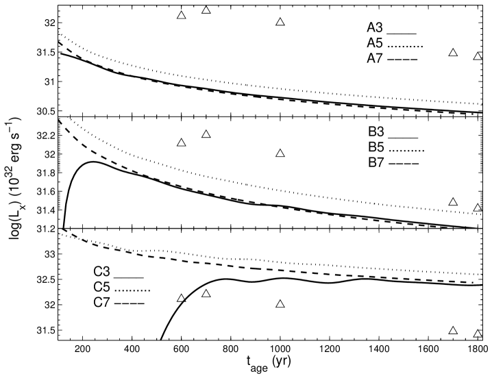
Figure 5: The luminosity as a function of the wind age $t={R_{c}}/{v_{c}}$, for all cases. The triangles mark the position on these plots of the five PNs listed in Table 2 (not including NGC 40). Note the different scales in the three panels.

Table 2: X-ray properties of Planetary Nebulae

#	PN	$L_{x}$	$T_{x}$	Dynamical Age
		$10^{32}$ erg s-1	$10^{6}$ K	yr
1	NGC 7027(PN G084.9-03.4)	1.3	3	600
2	BD +30 3639(PN G064.7+05.0)	1.6	3	700
3	NGC 6543(PN G096.4+29.9)	1.0	1.7	1000
4	NGC 7009(PN G037.7-34.5)	0.3	1.8	1700
5	NGC 2392 (PN G197.8+17.3)	0.26	2	1800
6	NGC 40 (PN G120.0+09.8)	0.024	1.5	5000

The parameters of the first four PNs are summarized by Soker & Kastner (2003). The data for NGC 2392 are from Guerrero at al. (2005), and for NGC 40 from Kastner et al. (2005).

4.2 Temperature

In order to further compare our results with observed PNs, we follow the evolution with time of the different runs in the temperature-luminosity plane. This enables us to analyze the three central, observed parameters: $L_{x}$, $T_{x}$, and $t$ simultaneously. The average temperature of the bubble $T_{x}$ at each time is calculated by equation (8) and the evolution of $L_{x}$ and $T_{x}$ are plotted in Fig. 6 for the various Runs. In a self-similar flow when cooling is neglected, the temperature of the bubble does not depend on time. However, in the present model, which includes the cooling effect, the average temperature does vary. At early times, when density is high and radiative cooling times are still short in the low-T regions of the flow (eq. 5), we do not include these regions for the computation of the average temperature. Consequently, the calculated average temperature at the early stages is higher than it is in the late-time self similar solutions. As the bubble expands and the density drops, cooling becomes less important and the temperature tends to the self similar solution as seen in Fig. 6.

It can be seen from Fig. 6 that the evolution tracks of the B Runs are most consistent with the observed PNs. This indicates that these Runs can reproduce the observed luminosities and temperatures. Out of the six PNs in the sample, three seem to lie between the B4 and B5 Run indicating a fast wind velocity of $v_{2}$ = 450–500 $~{}\rm{km}~{}{\rm s}^{-1}$, while the two youngest PNs are more consistent with a fast wind velocity of $v_{2}$ = 600 $~{}\rm{km}~{}{\rm s}^{-1}$. The oldest PN, NGC 40, is fitted better with even a slower fast wind, having a velocity of $\sim 450~{}\rm{km}~{}\rm{s}^{-1}$. This tendency of older PNs to be better fitted with slower fast winds indicates that the evolution with time of the properties of the fast wind blown by the central star should be considered. Such an evolution, namely, the increase in the fast wind speed and decrease of mass loss rate with time (e.g., Steffen et al. 1998; Perinotto et al. 2004), cannot be considered with a self similar solution.

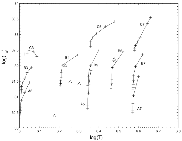
Figure 6: The evolution of the different cases with time in the temperature-luminosity plane. The $+$ signs mark radii along the track, from upper right to lower left, and in units of $10^{16}~{}\rm{cm}$: 1, 4, 7, 10, 13, 16, and 19. The triangles mark the position of the six PNs given in Table 2 on these plots.

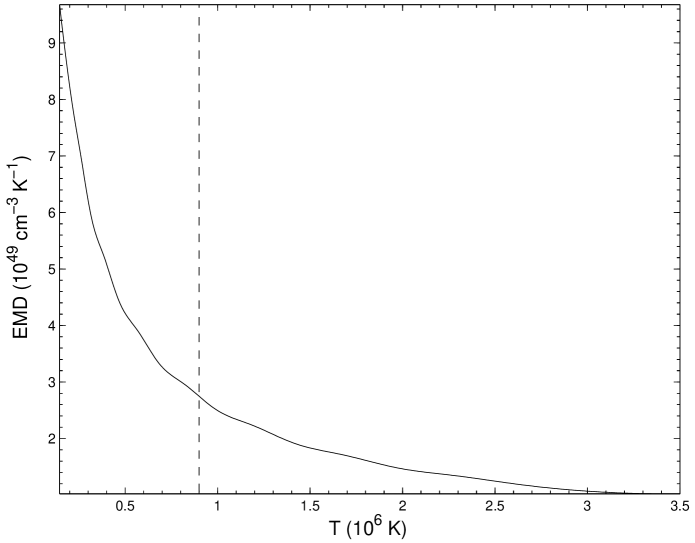
Figure 7: The emission measure distribution as a function of temperature for run B5 at the age 291 yr. The dashed vertical line is the cutoff for the cooling effect.

With the prospect of high spectral resolution X-ray observations of PNs, there is interest not only in the average temperature $T_{x}$, but also in the temperature distribution of the X-ray source, i.e., in the explicit form of $EMD(T)$ (see Eq. 10). This is the quantity that determines the emission-line details of the X-ray spectrum (along with the elemental abundances). From the self similar solution we have the explicit profile of $T(r)$, which can be easily transformed into $EMD(T)$. In Fig. 7, we plot $EMD(T)$ for the B5 Run at the age of 291  yr. It can be seen that $EMD(T)$ decreases sharply with temperature. This is why the observed (and calculated) $T_{x}$ values are all relatively low, only a few times 10⁶ K. Most of the gas in terms of emission measure is at low temperatures. The cutoff at low temperatures observed in Fig. 7 is somewhat arbitrary and is due to cooling. The lowest temperature gas cools rapidly below X-ray temperatures. Of course, in a more realistic, full hydrodynamic model this cutoff will be much more gradual. However, the effect of $EMD(T)$ peaking at low temperature $\sim$ 10⁶ K is expected to stay. The explicit forms of $EMD(T)$ calculated from the self similar solution can be used to predict the high-resolution spectra expected from future observations of PNs. No such spectrum is available yet.

4.3 Surface Brightness

When spatial resolution is sufficiently high and the number of photons is large enough, X-ray images of PNs can be obtained. In that case the image provides the surface brightness profiles. The normalized surface brightness is calculated from our models by integrating over the X-ray luminosity along the line of sight, chosen here as the $z$ direction, taken here at projected radius $d$ from the center of the bubble (see eq. 12)

$$S(d)=2\int_{0}^{\sqrt{R_{c}^{2}-d^{2}}}n_{e}n_{p}\Lambda_{0210}[T(z^{2}+d^{2})]dz.$$ (12)

The surface brightness profile as a function of projected radius $d$ is drawn in Fig. 8 for the B3, B5, and B7 Runs at ages of 300 yr and 1000 yr. The surface brightness rises sharply towards the contact discontinuity, but then drops rapidly just before reaching it. This is due to the efficient cooling in the high-density region right behind the contact discontinuity. The result is a bright X-ray region, which forms a ring close, but not touching, the contact discontinuity. In a full hydrodynamic calculation, the strongly emitting X-ray ring will be wider and the rise and drop of surface brightness will be more gradual than in Fig. 8. As was noted in the past, a bright X-ray ring is expected from a shocked central fast wind, but not from two fast jets (or a CFW). In NGC 40 an X-ray ring is observed, and a spherical wind seems to be present, as suggested by Kastner et al. (2005).

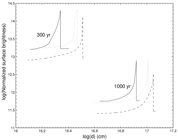
Figure 8: The surface brightness of the hot bubble after 300 year (left) and after 1000 year (right) for Runs B3 (solid), B5 (dotted), and B7 (dashed). Plotted from $R_{2}$ to $R_{c}$ with cutoff for $\tau_{\rm cool}<t$ .

4.4 Limitations of the Self Similar Approach

The self similar approach has several well known limitations. Here, we consider the two most important ones as far as the X-ray emission is concerned.

4.4.1 Time evolution

The inability to incorporate time evolution of the fast wind is indeed a limitation. However, our results show that this should not have a serious impact on the calculated X-ray flux and spectrum. The X-rays emanate predominantly from up-stream wind segments in the hot bubble, i.e., regions close behind the contact discontinuity (Fig. 8), that were expelled early and over a relatively short time period of $\sim 100-300~{}\rm{yr}$. The role of the wind blown later is merely that of a piston exerting pressure on the hot bubble from behind, and thus maintaining the high densities of the early-shocked gas. The contribution of these late-time wind segments to the X-ray emission is negligible as can be seen from Fig. 8.

In other words, according to our model, the details of the late-time evolution of the fast wind are not important to the X-ray emission as long as it continues to exert pressure on the high-density gas expelled earlier. Even if the gas in the inner regions of the hot bubble originates from a faster (say even, $v_{2}\sim\mathrm{few}~{}1000~{}\rm{km}~{}\rm{s}^{-1}$) and more tenuous wind, as expected for a more evolved post-AGB star, the over all PN X-ray emission would remain more or less as predicted by the self similar solutions, since the X-ray contribution of the tenuous, high-velocity wind segments is considerably less than that of the early up–stream segments.

4.4.2 Removing fast radiatively-cooling gas parcels

Another limitation of the present self similar approach is the approximate treatment of radiative cooling. As discussed in section 2.2, in the calculation of the X-ray emission, we did not include fast-cooling gas segments. We considered only the X-ray emission from gas segments with cooling times larger than the age of the nebula, namely, $\tau_{\rm cool}>t$. This, of course, is not a fully consistent treatment.

In order to test the sensitivity of our results to this assumption, we recalculated the X-ray evolutionary tracks of Fig. 6 for two cases, but now varying the criteria for eliminating the fast cooling gas. We chose the two runs, B4 and B6, most closely matching the observed PNs in Fig. 6, and we varied the threshold for including gas segments in the X-ray calculations from $0.25$ to $4$ times the age of the nebula. This reflects more than an order of magnitude uncertainty in the relevant cooling time (clearly more than enough). The results are plotted in Fig. 9. As can be seen from Fig. 9, including gas with extremely short cooling times (the lines marked $\tau_{\rm cool}>t/4$, i.e. overestimating the amount of X-ray gas) increases the calculated X-ray luminosity, while slightly reducing the average X-ray temperature (by a factor of $<10^{0.08}=1.2$). These effects are noticeable only when the nebula is very young. At higher PN ages the lines converge to the original $\tau_{\rm cool}=t$ result. Recall that the evolution in these tracks goes from high- to low- temperatures, the first point in each track corresponding to a contact discontinuity radius of $10^{16}~{}\rm{cm}$ and an age of only $\sim 100$ years. Since most PNe are observed at much older ages, this result implies that including fast-cooling gas does not have an appreciable effect on our results for the X-ray luminosity nor the average temperature.

Taking our criterion to the other extreme and including in the calculation of the X-ray emission only gas with very long cooling times ($\tau_{\rm cool}>2t,3t,\mathrm{and}~{}4t$, i.e., thus decreasing the amount of X-ray gas considered) produces evolutionary tracks generally to the right (higher-T) of the $\tau_{\rm cool}=t$ thick lines in Fig. 9. The result is to gradually reduce the X-ray luminosity and to increase the average X-ray temperature, as expected by eliminating more and more high-density, low-T segments. Ignoring the first point in each evolutionary track in Fig. 9 when the nebula is very young, the luminosity drops by a factor of $<10^{0.3}=2$, and the temperature rises by a factor of $<10^{0.08}=1.2$. This shows that even when we disregard all of the gas with cooling times much larger, by up to a factor of $4$, than the age of the nebula the results do not change by more than a factor of 2 in the most important measurable X-ray parameters. Only when we remove gas with cooling times as long as 5 times the nebular age (essentially ignoring the entire hot bubble) do we manage to reduce the X-ray luminosity much below the typical observed values. Removing gas with such long cooling times is clearly unjustified. Even removing gas with $\tau_{\rm cool}\sim 3t$ is not obviously justified.

To summarize this subsection, our main conclusion, that the observed X-ray emission of a large fraction of PNs can be accounted for by shocked wind segments that were expelled during the early PN phase when the fast wind speed is moderate, $v_{2}\sim$ 400-600 $~{}\rm{km}~{}{\rm s}^{-1}$, and the mass loss rate is a few times $10^{-7}M_{\odot}~{}\rm{yr}^{-1}$ holds. Our approximate treatment of the evolution of the fast wind and the exact radiative cooling scenario can not change these parameters by more than a factor of $\sim 2$. In the future, we hope to be able to carry out numerical simulations in order to study more closely the detailed processes responsible for the X-ray emission from PNe.

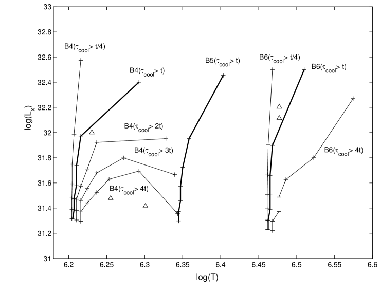
Figure 9: Evolution tracks as in Fig. 6, but only for models B4, B5, and B6, and here we examine different criteria for removing cooled regions from the computation of the X-ray emission. Thick lines show the results as in Fig. 6, namely, only regions with cooling times $\tau_{\rm cool}>t$ are included in the computation of the X-ray emission; $\tau_{\rm cool}$ is the radiative cooling time (eq. 3), and $t(=R_{c}/v_{c})$ is the age of the wind. The thin lines show the evolution of runs B4 and B6 obtained using different criteria for removing cooled regions. These are, as marked, $\tau_{\rm cool}>t/4$, $\tau_{\rm cool}>2t$, $\tau_{\rm cool}>3t$, and $\tau_{\rm cool}>4t$.

5 CONCLUSIONS

We use the self similar solution for the collision of two spherically symmetric concentric winds (CI83) to present a quantitative treatment of the X-ray emission expected from the shocked fast wind blown by the central stars of PNs and proto-PNs. We compare our results with five X-ray bright PNs for which high quality X-ray observations are available. The comparison constrains the parameter space of the physical quantities relevant to these PNs. With the assumptions made in our model, we find that the fast wind velocities of these PNs are between 400 and 600 $~{}\rm{km}~{}{\rm s}^{-1}$. Much higher or lower velocities can not produce the high X-ray luminosities observed. Furthermore, we find that for the observed PNs, the mass outflow rates in the fast wind under our assumptions, is of the order of a few $10^{-7}M_{\odot}~{}\rm{yr}^{-1}$, perhaps even reaching $10^{-6}M_{\odot}~{}\rm{yr}^{-1}$. Our results strengthen the claim of Soker & Kastner (2003; see Fig. 4 here), that the strongest contribution to the X-ray emission of the shocked fast wind blown by the central star comes from shocked wind segments that were expelled during the early PN phase when the wind speed was moderate $\sim 500~{}\rm{km}~{}\rm{s}^{-1}$. This is most clearly seen in Figures 5 and 6. As Soker & Kastner (2003), we also find that the fast wind can account for the luminosity and temperature of the X-ray emitting gas in PNs. However, the increase of the fast wind speed and decrease of the mass loss rate must be considered to get a better match to observations. This cannot be achieved with a self-similar solution.

It has been suggested that the relative low X-ray temperature in PNs results from heat conduction from the hot bubble to the cold shell (Soker 1994), or from mixing of the hot bubble and the cold shell material (Chu et al. 1997). The heat conduction process was studied recently in great detail by Steffen et al. (2005), who find that it can indeed account for X-ray properties of PNs. We do not claim that heat conduction does not occur, or that it cannot account for the X-ray properties of PNs. We rather argue that the X-ray properties of PNs can be explained with the evolution of the central star wind even if heat conduction is inhibited by magnetic fields. Future observations and their comparison with models based on heat conduction or wind evolution will determine the dominant cause of the low temperature of X-ray emitting gas in PNs.

We have also calculated the expected X-ray surface brightness (in relative units). In reality, where the fast wind evolves with time, the X-ray bright ring will not be so thin, and the X-ray emission will be spread on a wider ring. Still, the ring-shaped X-ray emission is a clear signature that the X-ray emitting gas comes from a spherically symmetric wind, and not from jets. This has been suggested to be the case in NGC 40 (Kastner et al. 2005). In some other PNs, such as He 3-1475 (Sahai et al. 2003) and Mz 3 (Kastner et al. 2003), the morphology of the X-ray emission clearly points at the presence of jets. This shows that in different PNs there might be different origins for the X-ray emitting gas, as noted by previous authors studying X-ray emission from PNs, e.g., Guerrero et al. (2005). Therefore, the X-ray emission can be used to shed light on the shaping process of PNs.

The self similar calculations includes the adiabatic cooling of the gas, which must be considered for comparison with observations (Soker & Kastner 2003). However, it does not include the radiative cooling. We have treated radiative cooling by not considering shocked-gas shells with radiative cooling times shorter than the age of the flow. The effect of removing fast cooling gas segments has been shown to be important only for the high-mass, low-velocity winds. The changing properties of the blown fast wind with time, radiative cooling of the shocked fast wind will be treated in a future paper where we will use a numerical code.