Amplification of Primordial Magnetic Fields by Anisotropic Gravitational Collapse
Abstract
If a magnetic field is frozen into a plasma that undergoes spherical compression then the magnetic field varies with the plasma density according to . In the gravitational collapse of cosmological density perturbations, however, quasi-spherical evolution is very unlikely. In anisotropic collapses the magnetic field can be a much steeper function of gas density than in the isotropic case. We investigate the distribution of amplifications in realistic gravitational collapses from Gaussian initial fluctuations using the Zel’dovich approximation. Representing our results using a relation of the form , we show that the median value of can be much larger than the resulting from spherical collapse, even if there is no initial correlation between magnetic field and principal collapse directions. These analytic arguments go some way towards understanding the results of numerical simulations.
keywords:
magnetic fields – cosmology: theory – large-scale structure of Universe – galaxies: formation – galaxies: clusters: general1 Introduction
One of the most significant gaps in our understanding of cosmological structure formation is how large-scale magnetic fields arise and how they relate to the processes involved in galaxy and cluster formation. The observed galactic fields, with typical strengths of a few G, could be the result of the amplification of a tiny seed field, perhaps small as G. On the other hand the adiabatic compression of a somewhat larger primordial field of G could also achieve similar strengths in bound objects without violating cosmological constraints. For general reviews of various aspects of cosmological magnetic fields, see Kronberg (1994), Widrow (2002) and Vallee (2004).
One specific situation where magnetic fields might prove important is in galaxy clusters. The most convincing line of evidence demonstrating the existence of magnetic fields in clusters emerges from studies of Faraday rotation measures (RM). Typical RM values of galaxy clusters are of the order of a few 100 rad/m2, roughly consistent with field strengths of a few G. These are comparable with galactic magnetic fields, but well below equipartition with the thermal cluster gas. Much larger RM values of a few 1000 rad/m2 have been detected in cooling-flow clusters, indicating possibly substantial magnetic pressure support of the intra-cluster gas there (e.g. Carilli & Taylor 2002). Although the magnetic fields of galaxy clusters are less ordered than those of spiral galaxies, the presence of coherent structures is suggested by high resolution Faraday maps (e.g. Dreher et al. 1987; Taylor & Perley 1993; Taylor et al. 2001; Eilek & Owen 2002). These structures could result from shear-amplification of originally small-scale magnetic fields, as is suggested by MHD simulations of galaxy cluster formation (Dolag et al. 1999). It is clear, however, that the overall power-spectrum of magnetic field fluctuations in clusters is rather broad ; see Dolag et al. (2002). The observed magnetic fields could play a significant role in supporting the intracluster medium through magnetic pressure (Loeb & Mao 1994) and there is some evidence that fields may be dynamically important in some clusters (Dolag et al. 2001; Eilek & Owen 2002). It is not known, however, how important these are or how they got there (Dolag et al. 1999; Goncavles & Friaca 1999; Dolag & Schindler 2000; Vlahos et al. 2005).
In this paper we look at the behaviour of a primordial magnetic field during cosmological evolution. Our aim is to develop an understanding of how gravitational collapse can, even in the absence of turbulence or other dynamo action, lead to a significant amplification of magnetic fields during the the evolution of clusters or other large-scale cosmic structures. The essence of our argument is very simple. Assume there is a primordial magnetic field in a region undergoing compression and that the field is frozen into the plasma in that region. Since flux is conserved, the magnetic field strength scales with the cross-sectional area of the collapsing region while the gas density scales with its volume. The net result for a spherical compression is that assuming no back-reaction of the field on the collapse (which we assume throughout this paper). One is tempted to infer that the “average” amplification due to collapse of a random set of density perturbations should be equal to this value. However, it has been known since the pioneering work of Zel’dovich (1970) and Doroshkevich (1970) that the generic collapse of cosmological perturbations is very anisotropic; see also Shandarin & Zelovich (1989). It is also true that the amplification of the –field is a non-linear function of the overall collapse factor. Put these two facts together with the realisation that averaging does not commute with non-linear operations and it is clear that the angle-averaged amplification of need not be close to the isotropic value. This argument was first presented by Bruni, Maartens & Tsagas (2003) who showed that there are possible collapse geometries that lead to a much larger boost in the –field than one would naively expect. There is some evidence that this may be observed in galaxy clusters through a large value of the slope of the relation: taking a model of the form it seems values of can be inferred (Dolag et al. 2001). The particular issue we are interested in tackling is what one can say about probabilities of these collapses and whether they lead to a significant effect after averaging over all possible collapse directions.
Of course there are a number of complicated astrophysical processes that could boost the magnetic field in a cluster: turbulent dynamo action and the expulsion of galactic -fields are just two examples. These are beyond the scope of existing numerical methods, as well as analytic modelling, but it is nevertheless important to understand how much of the observed behaviour of cluster magnetic fields can be explained using simple arguments like those we present here.
In the next Section we run through some basic definitions and simple examples of anisotropic collapse. In Section 3 we use an argument based on the Zel’dovich approximation to calculate the distribution of for freely collapsing fluid elements arising from Gaussian initial fluctuations.
2 Basics
Consider the effect of a general deformation of a fluid element. Define a deformation tensor, , representing the deformation of an infinitesimal fluid element of initial side lengths , such that
| (1) |
The deformation described by is illustrated for the 2-D case in Figure 1.
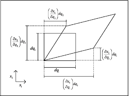
The initial co-moving volume of the fluid element, in three dimensions, is just , and its final comoving volume is , giving a ratio of final to initial volume of
| (2) |
The strength of a magnetic field is proportional to the density of its field lines. Hence, under the assumption that field lines are frozen into the fluid (as is usually assumed to be the case in astrophysical situations, due to the large scales involved), movement of the fluid perpendicular to the field lines affects the field strength, while movement parallel to the field lines leaves it unchanged.
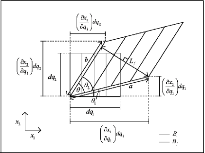
In order to see how the deformation tensor relates to the change in field strength it is easiest first to consider the two dimensional case, as illustrated in Figure 2. We first take the case where the initial field only. The strength of the magnetic field is proportional to the area (or in this 2-D case, length) perpendicular to the field lines. Hence in Figure 2,
| (3) |
We can find , the final length perpendicular to the field lines, by noting that
| (4) |
so from Equation 3 the magnitude of the final field, , is given by
| (5) |
since
| (6) |
and
| (7) |
and in two dimensions
| (8) |
Since the final field is no longer in the direction only we also need to know its and components, which are given by
| (9) |
and
| (10) |
Following the same route for a field which is initially in the direction only gives similar results, leading to total and components of the final field configuration given by
| (11) |
Extending this argument to three dimensions gives
| (12) |
The total magnitude of a magnetic field is given by
| (13) |
so in three dimensions the ratio of the magnetic field strengths before and after deformation is given by
| (14) |
In the case of isotropic collapse, , and all the off diagonal elements with are zero, giving
| (15) |
as expected, but the general case, which is not necessarily isotropic and can also include skew components, is more complicated than this.
This is all very well, but we need to set up a model that applies to collapses of fluid elements within a spatially varying random field of density perturbations. Let us assume, for a toy model, that each possible direction of collapse is independent and equally likely. It is then straightforward to work out the average amplification of the magnetic field which these deformations would produce. For reasons outlined in the introduction we focus on the parameter , where
| (16) |
We look first at the case of simple one–dimensional collapse, without skew components. If we assume that our initial magnetic field is in the direction only, then for collapse in the direction we have . The other diagonal elements , with all off–diagonal elements , which gives
| (17) |
so that in this case. For collapse in the or direction only we have, for each case,
| (18) |
In this case we see that .We will from now on work with averages obtained over all possible configurations of the deformation by associating a value of with each possible geometry and averaging these values. If these three eventualities discussed above are equally likely then the average value of , so that the average effect is , just as in the isotropic case.
We now look at the three possible skew directions, where the diagonal elements, , and one of the off–diagonal elements , with the other off–diagonal elements . When is the only non-zero off–diagonal element we have
| (19) |
so that . Similarly, when is the only non-zero off diagonal element we also find , but for the case where is non-zero, we find
| (20) |
Again we find that the average over these three possibilities is , as for the case of isotropic collapse.
However, in reality, each of these possible directions of collapse is not independent and equally likely. On the contrary, the elements of the deformation tensor are correlated, and as a consequence the amplification of the field is, on average, quite different from what would be expected from this naive model; see Bruni et al. (2003). In the next Section we investigate more realistic collapse geometries.
3 Realistic Collapse Models
3.1 The Zel’dovich Approximation
The Zel’dovich approximation (Zel’dovich 1970; Doroshkevich 1970; Shandarin & Zel’dovich 1989; Bartelmann & Schneider 1992; Sahni & Coles 1995) is an approach to structure formation which assumes that each particle has some small initial peculiar velocity which is determined by the initial density fluctuations. Particles then travel on ballistic trajectories determined by this initial veloicty, but unaffected by subsequent changes to the gravitational potential. Hence we write , the final (Eulerian) position of a particle at time , as
| (21) |
where is the scale factor of the universe, is the initial (Lagrangian) position of the particle, is the growing mode, which scales the peculiar velocity, , with time, and depends only the initial position . We can see that this equation looks like the background Hubble expansion, , plus some perturbation which vanishes as .
Changing to co-moving co-ordinates, , gives
| (22) |
If we assume that the initial velocity is irrotational (a reasonable assumption since it is generated by the gravitational effect of overdensities) we can write equation (22) in terms of a potential, , giving
| (23) |
where , and denotes differentiation with respect to the initial coordinates, . This equation looks very much like ballistic motion,
| (24) |
but with a peculiar time co-ordinate .
The Zel’dovich deformation tensor, , describes the deformation of a fluid element of initial side lengths , and is given by
| (25) |
where is the Kronecker delta and . The diagonal elements relate to the expansion and contraction of the fluid element along the principle axes, while the off-diagonal elements describe the skew distortion. The standard approach involves diagonalising the deformation tensor (which is symmetric). Let us denote the eigenvalues of by , so that the mass density becomes
| (26) |
where is the mean cosmological background density.
The Zel’dovich approximation describes the behaviour of evolving cosmological perturbations until the Jacobian in Equation (26) becomes zero, at which point the matter density becomes infinite and a caustic forms, where the mapping between Eulerian and Lagrangian coordinates is no longer unique. Although simple, the Zel’dovich approximation gives remarkably accurate results up to shell crossing (Coles et al. 1993). This, along with its natural formulation in terms of the deformation tensor describing the collapse of each fluid element, makes it an ideal approach for studying the effect of gravitational collapse on magnetic field strength.
3.2 Probabilities
The joint probability density function (JPDF) for the elements of the Zel’dovich deformation tensor is given by Doroshkevich (1970), where a very elegant discussion is also presented about the probability of various collapse geometries. The most likely collapse is initially along one direction, resulting in caustics that are generically two–dimensional (“pancakes”). To proceed we assume the initial density perturbations are Gaussian, as is expected from inflationary models (Bardeen et al. 1986). The initial velocity potential is then also Gaussian, and so are its derivatives. Therefore the JPDF of the second derivatives of the velocity potential, on which the elements of the deformation tensor depends, is a multivariate Gaussian distribution. If we write all the possible second derivatives as a vector, , , with the diagonal elements, which have , as , , and the off–diagonal elements with as , , , then their joint probability is given by
| (27) |
and we need only find the value of the covariance matrix, , to know the probability distribution in full. Note that all the variates involved have zero mean. The components of are given by
| (28) |
where
| (29) |
if is the power spectrum. So we now know the multivariate Gaussian distribution which gives the JPDF of the elements of the deformation tensor, provided we know , the power spectrum of the initial density perturbations. For simplicity we take the case where the magnetic field is entirely independent of the deformation tensor (i.e. we are not appealing to the field to create the initial deformation in any way, so there is no correlation between the field and the deformation), and ignore any back reaction of the field on the fluid. This gives us the freedom to choose to have the initial magnetic field along one axis, eg only. This simplifies the equation for the field strength amplification (Equation 14) considerably, giving
| (30) |
Since the marginal distribution , the probability distribution of the magnetic field amplification, given the deformation tensor, is given by
| (31) |
where
| (32) |
and is the Dirac delta-function. Similarly, the the density compression factor is
| (33) |
and its probability distribution is
| (34) |
The two distributions (31) and (34) are both skewed showing that there are amplifications and compressions much larger than average. This skewness also increases with time, as the perturbations become more non-linear. This suggests that there is a significant probability of large amplifications of relative to , as suggested by Bruni et al. (2003). However these two distributions are not sufficient to calculate the distribution of our chosen parameter , which we define by
| (35) |
which requires the full joint distribution . Unfortunately the integrals involved in the construction of this joint distribution are resistant to analytical methods. In order to investigate the statistical properties of (where ), we therefore resorted to numerical techniques.
3.3 Calculations
Although the multivariate distributions described above are difficult to handle analytically, it is fortunately quite easy to obtain the distribution of using a Monte Carlo technique. First we need to generate deformation tensors from the distribution (27). One can generate correlated Gaussian variates with a given covariance matrix by simply reversing the process by which one can diagonalise the covariance matrix to produce independent variates from correlated ones. In other words, we start with a set of six independent and identically distributed Gaussian variables, and then construct a linear combination such that they produce the correct covariance matrix. This is easily done using a Cholesky decomposition. We use this technique to generate a large library of deformation tensors that constitute a fair sample from the required distribution (27). We then used the machinery described above to calculate the compression factors and from this sample. This in turn generates a value of for each fluid element from which the overall distribution can be formed. For simplicity we have assumed, as before, that there is no correlation between the magnetic field and the deformation, and have ignored any back reaction of the magnetic field on the fluid.
There are a number of subtleties that must be confronted before dealing with this distribution. The first is that not all deformation tensors compatible with our parent distribution lead to collapsing fluid elements. Since we wish to look at collapsed regions only, we consequently restrict our library of deformations describing a net compression in comoving coordinates. Secondly, since our variates are Gaussian the eigenvalues are also Gaussian, Equation (26) always assigns a non-zero value to regions where shell–crossing has occurred. This generates a tail in the distribution that is unphysical. For this reason we illustrate our results by focussing on the field strength amplification which would be generated by a freely collapsing fluid element whose overdensity, , has reached a value
| (36) |
Each fluid element in our library was allowed to collapse to this state, at which point the magnetic field compression factor, , which depends strongly upon the exact configuration of the collapse, was determined using methods given in Section 2. This was then compared to the change in density to find a value of for each element. These values were binned to give final distributions of and which can be seen in Figures 3 and 4, respectively. Notice that the distributions of both B and have a very long tail of values. This effect is understandable in terms of a simple model: if a fluid element collapses in directions orthogonal to the magnetic field, the field obviously undergoes a large boost. However, it is possible for the fluid element to be expanding along the third direction (along the field). This means that can increase significantly while hardly changes at all. This can lead to unbounded values of . These are unlikely, but not impossible so they have a finite probability. The mean value of is consequently formally undefined.
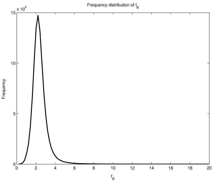
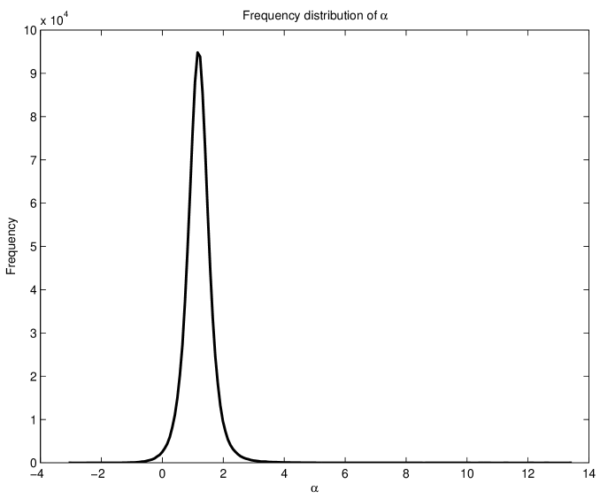
Intriguingly, the median value of once all the fluid elements had collapsed until , is found at a value of , considerably higher than the expected isotropic value of . One has to be careful interpreting this result as it does not correspond to a calculation of at the same epoch. Some fluid elements will reach at different times to others. Since the background and the background the initial ratio effectively depends on the time taken to collapse through or, equivalently as . To compare these results at the same epoch one should therefore subtract from the result above giving .
While most deformations cause a field amplification at or near the median value (approximately 87% are within 50% of the median), there are some outliers caused by unusual alignments of the magnetic field compared to the direction of greatest collapse as discussed above. High values of are caused by configurations where the collapse of the deformation tensor is such that the magnetic field is amplified greatly for only a small change in the density. This occurs when the magnetic field is perpendicular to the axis of fastest collapse, and parallel to an axis along which the collapse is slow, or expansion is occurring. On the other hand, if this happens the magnetic field may reach such a large level that it begins to exert a back-reaction on the collapse. Our treatment can not handle this eventuality accurately.
Similarly, extremely low values of , some of which are negative, occur when the field is perpendicular to an axis which is collapsing slowly, or even expanding, and parallel to a quickly collapsing axis, causing a large increase in density for very small increase, or even a decrease, in magnetic field strength. Such alignments are unusual, but do occasionally occur, and cause the long tails in the distribution of seen in Figure 4.
4 Discussion
We have investigated the probable magnetic field amplification by anisotropic gravitational collapse under a number of restrictive assumptions. These are:
-
1.
the initial fluid perturbations are Gaussian;
-
2.
the initial magnetic field is uncorrelated with the perturbations;
-
3.
collapse is described by the (quasi–linear) Zel’dovich approximation;
-
4.
shell-crossing does not occur;
-
5.
there is no back-reaction of the magnetic field on the fluid motion.
We find the median value of to be significantly higher than the isotropic value of , but the precise value depends on exactly how one performs averages. We have taken two definitions (which differ by in ) but other ways of averaging are possible. Indeed, for comparison with a single cosmological object one would probably have to average over correlated fluid elements, and average by mass rather than by direction. Obviously if one averages over coherent structures and/or if there are correlations between magnetic field and the fluid perturbations, such as would be the case if the field were generated by fluid activity, then the results would be very different.
In the numerical simulations presented by Dolag et al. (2001) it seems values of can be reached. We cannot argue that our simplified treatment can be compared directly with these more accurate computations, but it is reassuring that taking proper account of collapse geometries leads to plausible values of that are not far from those reached in fully MHD approaches. This suggests at any rate that it may be possible to get some insight into the behaviour of cluster magnetic fields using simple arguments like those we have presented here, without needing to appeal to more complex mechanisms such as sheer flows and dynamos.
References
- [1] Bardeen J.M., Bond J.R., Kaiser N., Szalay A.S., 1986, ApJ, 304, 15
- [2] Bartlemann M., Schneider P., 1992, A&A 259, 413
- [3] Birk G.T., Wiechen H., Otto A., 1999, ApJ, 518, 177
- [4] Bruni M., Maartens R., Tsagas C.G., 2003, MNRAS, 338, 785
- [5] Carilli C.L., Taylor G.B., 2002, ARA& A, 40, 319
- [6] Coles P., Melott A.L., Shandarin S.F., 1993, MNRAS, 260, 765
- [7] Dolag K., Bartelmann M., Lesch H., 1999, A& A, 348, 351
- [8] Dolag K., Bartelmann M., Lesch H., 2002, A& A, 387, 383
- [9] Dolag K., Schindler S., 2000, A& A, 364, 491
- [10] Dolag K., Schindler S., Govoni F., Feretti L., 2001, A& A, 378, 777
- [11] Doroshkevich A.G., 1970, Astrofizika, 6, 320
- [12] Dreher J.W., Carilli C.L., Perley R.A., 1987, ApJ, 316, 611
- [13] Eilek J.A., Owen F.N., 2002, ApJ, 567, 202
- [14] Goncalves D.R., Friaca A.C.S., 1999, MNRAS, 309, 651
- [15] Kronberg P.P., 1994, Rep. Prog. Phys., 57, 325
- [16] Loeb A., Mao S., 1994, ApJ, 435, L109
- [17] Röttiger K., Stone J.M., Burns J.O., 1999, ApJ, 518, 594
- [18] Sahni V., Coles P., 1995, Phys. Rep., 262, 1
- [19] Shandarin S.F., Zel’dovich Ya. B., 1989, Rev. Mod. Phys., 74, 775
- [20] Taylor G.B., Govoni F., Allen S.W., Fabian A.C., 2001, MNRAS, 326, 2
- [21] Taylor G.B., Perley R.A., 1993, ApJ, 416, 554
- [22] Vallee J.P., 2004, New Astr. Rev., 48, 763
- [23] Vlahos L., Tsagas C.G., Papadopoulos, D., 2005, ApJ, 629, L9
- [24] Widrow L.M., 2002, Rev. Mod. Phys., 74, 775
- [25] Zel’dovich Ya.B., 1970, A&A, 5, 84