VLBI phase–reference observations of the gravitational lens JVAS B0218+357

We present the results of phase–referenced VLBA+Effelsberg observations at five frequencies of the double–image gravitational lens JVAS B0218+357, made to establish the precise registration of the A and B lensed image positions. The motivation behind these observations is to investigate the anomalous variation of the image flux–density ratio (A/B) with frequency – this ratio changes by almost a factor of two over a frequency range from 1.65 GHz to 15.35 GHz. We investigate whether frequency dependent image positions, combined with a magnification gradient across the image field, could give rise to the anomaly. Our observations confirm the variation of image flux–density ratio with frequency. The results from our phase–reference astrometry, taken together with the lens mass model of Wucknitz et al. (2004), show that shifts of the image peaks and centroids are too small to account for the observed frequency–dependent ratio.

1 Introduction

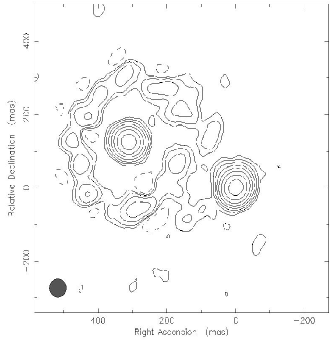
Figure 1: A combined EVN/MERLIN 1.7 GHz map of B0218+357, observed on  $29^{\textrm{th}}$ May 1997 (Patnaik et al., unpublished). The resolution of the map is 50 mas and it shows an Einstein ring and the two compact images, A (right) and B (left). The contour levels are 6.5 mJy $\textrm{beam}^{-1}\leavevmode\nobreak\ \times(-0.5,0.5,12,4,8,16,32,64)$ and the peak flux–density is 650 mJy $\textrm{beam}^{-1}$.

Table 1: The image flux–density ratios as a function of frequency. S${}_{\textrm{A}}$ and S${}_{\textrm{B}}$ denote flux–densities of image A and B, respectively. Entries marked with an * indicate MERLIN and VLA measurements free from contamination by the Einstein ring. The error bars are included where available.

$\nu$ (GHz)	Interferometer	Resolution (mas2)	S${}_{\textrm{A}}$ (mJy)	S${}_{\textrm{B}}$ (mJy)	$\quad\textrm{S}_{\textrm{A}}/\textrm{S}_{\textrm{B}}$
1.7	VLBIa	5$\times$5	445$\pm$23	170$\pm$9	2.62$\pm$0.19
$5^{*}$	MERLINb	50$\times$50	728$\pm$15	245$\pm$5	2.97$\pm$0.09
$4.84^{*}$	VLAc	400$\times$400	880$\pm$80	370$\pm$20	2.38$\pm$0.25
5	EVNb	5$\times$5	660	210	3.14
5	VLBIa	1$\times$1	515$\pm$26	196$\pm$10	2.62$\pm$0.19
$5^{*}$	MERLINb	50$\times$50	694$\pm$14	215$\pm$5	3.23$\pm$0.10
$8.4^{*}$	VLAb	200$\times$200	767	236	3.25
$8.4^{*}$	VLAd	200$\times$200	847	235	$3.57\pm 0.01$
$8.4^{*}$	VLAc	220$\times$220	807$\pm$40	271$\pm$15	2.98$\pm$0.22
$15^{*}$	VLAd	120$\times$120	935	570	$3.73\pm 0.01$
$15^{*}$	VLAb	120$\times$120	698	189	3.69
$22.4^{*}$	VLAc	96$\times$76	833$\pm$160	253$\pm$50	3.29$\pm$0.90

The radio source JVAS B0218+357 was identified as a gravitationally lensed system by Patnaik et al. (1993). The source (Figure 1) consists of two compact images, A and B, separated by $\sim$330 mas, the smallest angular separation amongst the known galaxy lenses, and a faint Einstein ring of a similar diameter. Optical observations of the lens (Browne et al. 1993; Stickel & Kuhr 1993; O’Dea et al. 1992) have revealed molecular absorption lines associated with the lens galaxy at the redshift of 0.684. The morphology of the lens galaxy is spiral as suggested by the large differential Faraday rotation ($\sim 900$ rad $\textrm{m}^{-2}$) which is measured between the images (Patnaik et al. 1993) and detections of radio molecular absorption lines (Wiklind & Combes 1995; Carilli et al. 1993) indicating that the lens–galaxy is rich in ionized gas, common to late–type spirals. The small image separation, which is indicative of a low–mass galaxy acting as a lens, lends support to this morphological categorization. The background source has properties of a powerful radio source and a red optical continuum (Stickel & Kuhr 1993), based on which it is conjectured to be a blazar, and its redshift has been confirmed using optical spectroscopy (z $=$ 0.944, Cohen et al. 2003; Browne et al. 1993). Further, it is variable in its radio emission and an accurate value for the time delay between variations in the images has been measured by Biggs et al. (1999), (10.5 $\pm$ 0.4) days (see also Cohen et al. 2000).

Previous VLBI observations at high frequencies (Biggs et al. 2003; Kemball et al. 2001; Patnaik et al. 1995) show that both images consist of a compact core component and a secondary compact component, offset by ca. 1.5 mas in the direction of a lower brightness jet of some 15 mas extent. At lower frequencies (e.g. Porcas & Patnaik 1996) the resolution is insufficient to separately resolve the two compact components but the total extent of both images increases considerably with increasing wavelength. In particular, image A, the stronger and larger, is extended in PA $-40^{\circ}$, the expected direction of “tangential stretching”.

The wealth of data coming from numerous radio and optical observations of this system at various frequencies and epochs provides constraints for lens models and, together with the time delay, give the possibility to determine the Hubble constant, $H_{0}$. This has been accomplished by various groups. Biggs et al. (1999) obtained a value of $H_{0}=69^{+13}_{-19}$ km s^-1 Mpc^-1 using a singular isothermal elliptical (SIE) mass distribution and Wucknitz et al. (2004) obtained a value of $H_{0}=78^{+6}_{-6}$ km s^-1 Mpc^-1 using a SIE potential (SIEP). The only problem in $H_{0}$ determination is related to the fact that the lens galaxy has weak optical emission, and is almost completely masked by the emission from image B (which is brighter than its counterpart in the optical wavebands). Thus, the position of the lens galaxy is poorly known relative to the lensed images and has been taken as a free parameter by the earlier authors in their (respective) lens models. A direct attempt to extract the optical centre of the lens–galaxy has been made by York et al. (2005) who after subtracting the emission from the images, A and B, describe the lens centre as a point about which the residuals are most symmetric. From their observations alone and using a SIEP lens model, they derive $H_{0}=66^{+9}_{-9}$ km s^-1 Mpc^-1 or $H_{0}=79^{+7}_{-7}$ km s^-1 Mpc^-1 depending upon whether the spiral arms of the galaxy are masked or not.

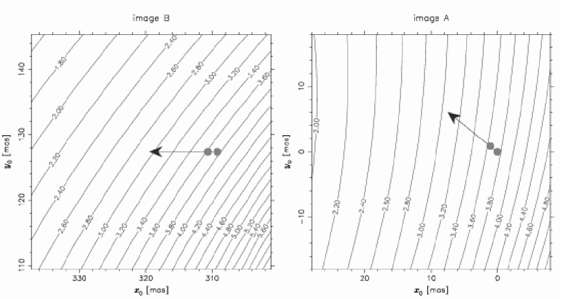
Figure 2: The curves indicate constant relative magnifications (A/B) for the best fitting lens model with the lens position at $x_{o}=260$ mas and $y_{o}=117.5$ mas (Wucknitz 2002). The filled circles represent the sub–components, 1 (west) and 2 (east), and the arrows represent the expected direction of the shift in the centroid of the brightness distribution of the images at lower frequencies, i.e. towards sub–component 2 which forms the base of the radio–jet.

Even though the basic lensing characteristics of this system are well–understood and well–reproduced by the current lens models, there are a few complications. One of them is the steady and systematic decline in the ratio of radio image flux–density of the A and B images with decreasing frequency. This is in direct contradiction to the expected achromatic behaviour of gravitational lensing for point sources. Table 1 lists the observed ratios from previous observations of B0218+357 at various frequencies and times, and using different interferometric instruments. The ratio (A/B) varies from 3.7 to 2.6 over the frequency range 15.35 GHz to 1.65 GHz. At frequencies where the source is variable, the ratio measured at a single epoch will be in error if the timescale for significant variations is comparable with the time delay. The three–month VLA monitoring of B0218+357 at 15 GHz and 8.4 GHz by Biggs et al. (1999) has revealed variations in the image flux–densities on a timescale of (70–100) days. This, along with the measured time–delay between the images, can induce variations in the ratio at the level of (10–11) %. This is in good agreement with the 15 GHz ratios of the image flux–densities measured at the same epoch which fall in the range from 3.45 to 3.96, with the mean value of 3.74 and an rms of 0.02. At 8.4 GHz, the level of the observed variation in the ratio reduces to (7–8) % and the rms reduces to 0.01. It is indeed expected that the variability amplitude of the background radio source reduces with frequency as the contribution from non–variable radio components becomes larger. Hence, although the time–variability in the background source emission along with the time–delay between the lensed images results in a spread of the estimated image flux–density ratios at a given frequency, it is clearly not the cause of the observed chromaticity in the flux–density ratio.

We note that interferometric measurements may underestimate the individual image flux densities if the beam size is much smaller than the extent of the image. If this occurs preferentially in one of the images it will affect the flux–density ratio; since image A is larger than image B, this effect might decrease the A/B flux–density ratio. Conversely, insufficient resolution may lead to contamination of the B image by emission from the Einstein ring. We have included entries in Table 1 from short baseline instruments (VLA, MERLIN; marked with an ‘*’) only at frequencies where the resolution is sufficient to separate the ring emission from image B, to minimize this effect.

Although gravitational lens imaging of a point object is intrinsically achromatic, frequency dependent variations in the image flux–density ratio of an extended source are possible, provided its structure changes as a function of frequency and extends over regions of different relative magnifications. It seems quite possible that this occurs in B0218+357 since both conditions exist. Firstly, the small image separation leads to relative large changes in magnification across the extent of the images. For simple isothermal ellipsoid models of the lens potential, a shift of 15 mas in the position of a point–source image can produce a change in relative magnification from 4 to 2.5 (see Figure 2).

Secondly, the frequency–dependence of the B0218+357 image structures is strong, with previous VLBI observations showing a marked increase of image sizes with decreasing frequency. Furthermore, it is common for the radio spectra of one–sided AGN jets such as that seen in B0218+357 to steepen with distance from the nucleus, providing a natural mechanism for producing a frequency–dependent position. The position of the radio peak at the base of the jet is also expected to move away from the nucleus at lower frequencies – the “core–shift”.

However, instrumental limitations prevent these effects from being seen easily. One is the change with frequency of the resolution available from VLBI observations. Another is the loss of absolute position information when phase self–calibration is used to make VLBI maps, which prevents robust registration of maps at different frequencies. Frequency–dependent position shifts should, in general, show up as a change with frequency of the separation between different images (e.g. Porcas & Patnaik 1995). However, such differential shifts are hard to measure in some cases, especially when the shift is in the same direction in both images. Furthermore, any “feature” (e.g. the core) used to define the positions of the different images may, in fact, include different fractions of the emission in the background source, since the images have different magnifications

In this paper we present the results of phase–referenced VLBI observations of the lensed source B0218+357, made to establish an unambiguous registration of the structures of the radio images at different frequencies. Although the expected core shifts are relatively small (mas), the positions of the centroids of the image flux–density distributions may change with frequency by larger amounts, and these are more representative of the position of the emission. It is therefore important to quantify their changes with frequency when investigating the origin of the frequency–dependent image flux–density ratios.

2 Inverse phase–referencing

VLBI observations suffer from the corrupting influence of the troposphere, ionosphere and instrumental uncertainties on the interferometer visibility phase. It is well–known that the use of phase self–calibration to eliminate these errors results in loss of the geometrical phases which contain information regarding the source position relative to the antennas, resulting in the loss of any information on the source position in the sky.

Alternatively, the technique of phase–referencing (Alef 1989) can be used, wherein observations of the target and a reference source are alternated frequently, allowing mapping of the target and determination of its position with respect to the reference. If the reference source is sufficiently compact that its position is achromatic, it can be considered as an astrometric calibrator. Then, the phase–reference observations can be used to make a correct registration of maps of the target source at different frequencies, to study any frequency–dependent structure.

Although this technique is most often used for mapping faint radio sources, the target in our study, B0218+357, is sufficiently strong ($\sim$ 1 Jy) that we can use “inverse phase–referencing”. Here, the target is used as the phase–reference for determining the corrupting phases, and phase–reference maps of a point–like, achromatic astrometric reference source are made. One advantage is that relatively faint sources can be used as astrometric references, permitting the choice of sources closer to the target, which minimizes telescope drive times and reduces any difference between the tropospheric and ionospheric phase corruptions of the target and reference. Another advantage is that multiple astrometric reference sources can be used to guard against the possibility that any single one may have chromatic structure.

3 Observations

VLBI observations were made at five frequencies, 15.35 GHz, 8.40 GHz, 4.96 GHz, 2.25 GHz and 1.65 GHz, using the NRAO Very Long Baseline Array (VLBA) and the Effelsberg radio telescope (Eb). Two 14 h source tracks were used ($13^{\textrm{th}}$ to $14^{\textrm{th}}$ and $14^{\textrm{th}}$ to $15^{\textrm{th}}$ January, 2002) and for each track (19 h to 03 h UT for Eb, 19 h to 09 h UT for the VLBA) we switched between two receivers every 22 min. For the first track, observations were alternated between 4.96 GHz and 2.25 GHz/8.40 GHz (S and X dual band) using 1 bit sampling, and for the second track between 1.65 GHz and 15.35 GHz (without Eb) using 2 bit sampling. The data were recorded on four 8 MHz basebands at all the frequencies with the exception of eight basebands at 4.96 GHz. All observations were made in a single (LHC) circular polarization mode, except the dual S/X observations which were made in RHC.

Apart from observing B0218+357, three compact reference sources were observed (see Table 2) along with a fringe finder, B0234+285. Scans on B0218+357 of 1 min 20 s duration were interleaved by scans of 2 min duration on each of the calibrators in succession. The position reference sources were selected from the NRAO VLA Sky Survey (NVSS) catalogue. From an initial sample of candidate sources, these three were found to exhibit flat spectra and the most point–like structure on the basis of EVN and MERLIN 5 GHz observations (Porcas 2001). They all lie within two degrees of B0218+357 and are stronger than 25 mJy at both 1.4 GHz and 5 GHz, with spectral indices flatter than $-0.47$ (where the flux density, S $\propto\nu^{\alpha}$; $\nu$ being the frequency and $\alpha$ the spectral index) .

The data were correlated at the VLBA correlator, with an output averaging time of 2.1 s and a frequency resolution of 0.5 MHz, and further processed in AIPS, the Astronomical Image Processing Software package provided by NRAO.

Table 2: The position references, their separations from B0218+357, the correlated flux density on the short EVN baselines (S–EVN) and on the long EVN baselines (L–EVN) at 5 GHz. The ratio L/S is a measure of source–compactness.

Source name	Separation	S–EVN	L–EVN	L/S
	(degrees)	(mJy)	(mJy)
NVSS B0210+366	2.03	127	85	0.66
NVSS B0215+364	1.03	140	86	0.61
NVSS B0222+369	1.30	151	91	0.61

Figure 3: The top and bottom panels show 1.65 GHz, 2.25 GHz, 4.96 GHz, 8.40 GHz and 15.35 GHz maps of images A and B respectively, with frequencies increasing from left to right, top to bottom. The origin (0,0) is defined by the position of the peak intensity found in the initial run of fringe–fitting. This is the centre of A at all frequencies except for at 1.65 GHz at which the peak is in image B, entailing a reversal in the labeling of the axes. The residual noise in the maps is $\leq$ 500 $\mu$Jy $\textrm{beam}^{-1}$. The restoring beams used are (7, 5, 2, 1, 0.5) mas in the order of increasing frequency. The images clearly manifest all the earlier observed lensing–characteristics. Image A is tangentially stretched at a PA $\sim$ $-40\,^{\circ}$ and image B seems to be tangentially compressed. At 8.4 GHz and 15.35 GHz the images reveal further substructure, sub–components 1 and 2 with $\sim$ 1.4 mas separation, representing the core–jet morphology of the background source.

4 Data analysis and maps

(a)

(b)

(c)

Figure 4: Maps of 0215+364 at 2.3 GHz. a) Inverse phase–referenced map with ionospheric phase calibrations applied to the data. b) Without ionospheric phase calibrations. Both the maps are plotted with a 5 mas restoring beam and with identical contour levels at multiples of 3 mJy. c) Hybrid map obtained by means of self–calibration.

Table 3: The image flux–density ratios from this data set. $b$ denotes the resolution and $\sigma$ is the root–mean–square noise in the maps.

$\nu$ (GHz)	b (mas)	$\sigma$ (mJy/beam)	Flux Density:$\quad\textrm{S}^{A}$ (mJy)	Flux Density:$\quad\textrm{S}^{B}$ (mJy)	$\quad\textrm{S}^{A}/\textrm{S}^{B}$
1.65	50	0.35	$504\pm{9}$	$249\pm{5}$	$2.02\pm{0.05}$
2.25	50	0.48	$646\pm{16}$	$243\pm{7}$	$2.67\pm{0.10}$
4.96	30	0.25	$650\pm{9}$	$217\pm{3}$	$3.00\pm{0.06}$
8.40	10	0.50	$681\pm{8}$	$206\pm{8}$	$3.31\pm{0.13}$
15.35	5	1.00	$661\pm{5}$	$171\pm{6}$	$3.87\pm{0.14}$

Figure 5: a) Image flux–densities obtained from these observations. b) Image flux–density ratio from these observations (with cross symbols and dashed error bars) and previous observations (with plus symbols and solid error bars, see Table 1).

An essential step in the reduction of phase–reference data concerns the assumption of similar tropospheric and ionospheric phase errors for the reference and the target source. For VLBI observations the extra paths through the troposphere and ionosphere are very different for different antennas, especially because the source is seen at different elevations. The mean phase errors due to the troposphere, which scale as $\lambda^{-1}$, can be estimated approximately for each antenna, and are taken into account in the model used for correlation. The mean phase errors due to the ionosphere, which scale as $\lambda$, are highly unpredictable, however, and thereby prohibit the use of any model at the time of correlation. Since the errors become pronounced at long wavelengths, it is necessary to apply phase corrections from an ionospheric model after correlation. In applying the ionospheric and tropospheric models, it is only the mean phase offset that is removed for every antenna. The terms corresponding to small–scale temporal and spatial fluctuations still remain and it is hoped they are the same for the target and the reference source. For these observations, we used the AIPS task TECOR to apply an ionospheric model, produced by the Jet Propulsion Laboratory (JPL), and which gives an estimate of the total electron content as a function of longitude, latitude and time (for more details see Walker & Chatterjee 1999).

In the further analysis standard reduction procedures were used, applying amplitude calibration derived from telescope radiometry measurements and using fringe–fitting, self–calibration, CLEAN deconvolution procedures and mapping. As mentioned earlier, B0218+357 is sufficiently strong that self–calibration procedures could be applied at all frequencies. Hybrid maps were made by cleaning two sub–fields simultaneously, one for image A and the other for B. After initial maps had been obtained the fringe–fitting was repeated using these as an input model, and the mapping was repeated. Full resolution hybrid maps of both A and B images at all five frequencies are shown in Figure 3.

All three reference sources also proved to be strong enough to use phase self–calibration, and hybrid maps were therefore also made for these. On inspection, two of these sources were deemed to be unsuitable as position references. For B0210+366 the flux density drops to about 30 mJy at 1.6 GHz and consequently the position of the emission peak is not well defined. The maps of B0222+369 reveal a jet like feature at 2.3 GHz and 1.6 GHz, casting doubt as to whether the position of the peak is achromatic. Therefore for further analysis only B0215+364 was used as a position reference; it appeared point–like in the maps at all frequencies. An amplitude self–calibration procedure was used on this source to determine corrections to the a priori amplitude calibration, and these were then applied to the B0218+357 data to improve the maps.

Phase–reference maps of B0215+364 were made at all frequencies by applying the self–calibration solutions obtained from B0218+357 to the B0215+364 data. The dynamic range of these maps is poor and deteriorates with increasing frequency from 30:1 to 2:1 with rms noise $\sim(1-1.5)$ mJy. To investigate the efficacy of the ionospheric model we compared phase–referenced images made with and without ionospheric phase corrections. One such comparison can be seen in Figure 4 which shows maps of B0215+364 at 2.25 GHz. The peak flux per unit beam is almost 1.5 times higher if an ionospheric model is used [Figure 4(a)]. Moreover the peak positions differ by almost half a milliarcsecond. We conclude that even though the rms deviation in the total electron content measured by different groups is on the order of 25 %, the effect of applying any of the models is in the direction that improves the results.

5 Results

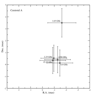
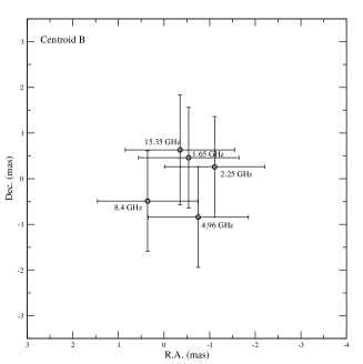
Figure 6: The change in the centroid position relative to the position–reference B0215+364, at five frequencies in image A (top) and image B (bottom). The error bars at 1.65 GHz, 2.25 GHz and 4.96 GHz are dominated by the position uncertainty in the B0218+357 maps due to the use of relatively large beams, and at 8.4 GHz and 15.35 GHz due to the position uncertainty of B0215+364 caused by the poor dynamic range of the phase–referenced maps at these frequencies.

The image flux–densities and flux–density ratios from these observations are presented in Table 3. To guard against loss of flux density due to over–resolution, we made low–resolution maps by discarding data from the longest baselines (using u,v resolution cut–offs). The flux densities from these maps were estimated by putting a box around the images and integrating the flux density within the box. The errors on the integrated flux–densities given in the table are derived from examining the spread in estimates obtained by varying a number of parameters in the imaging process, and are larger than the formal errors obtainable from a Gaussian fit. Shown in Figure 5(a) are the image spectra and it can be seen that image A flux–density remains almost constant (to within $\pm$ 25 mJy) at the upper four frequencies but drops suddenly by about 130 mJy (20 percent) at 1.65 GHz. In contrast, image B shows a gradual, monotonic increase with wavelength with no sharp drop. We note that the variation of the image flux–density ratio, as shown in Figure 5(b), is similar in trend to that found for previous observations , although the range is even larger ($\sim$ 4 to $\sim$ 2), with the value at 1.65 GHz differing most from previous estimates.

The result of the phase–referenced observations is shown in Figure 6, which shows the variation with frequency in the centroid position of the radio emission in the images with respect to B0215+364. To determine an image centroid position, the CLEAN components were convolved with a low–resolution restoring beam, and the peak in the resulting map was located using AIPS task MAXFIT, which fits a quadratic function to the brightest area of the map to determine the position offset with respect to the map centre. The same procedure was used to locate the offset from the map centre of the peak position of the calibrator, 0215+364, but using a full–resolution, phase–referenced map. The position of the B0218+357 image centroid with respect to 0215+364 (ignoring the constant position difference used for correlation) is then given by the difference of these offsets (B0218+357 – 0215+364). The same procedure was used for image B. The upper panel of the figure indicates a relative shift of $\sim 5$ mas in the centroid of image A between 15.35 GHz at 1.65 GHz, although the shift occurs only at 1.65 GHz. For image B, on the contrary, there is no shift detected in the centroid of the brightness distribution. From the Singular Isothermal Elliptical Potential (SIEP) model (Figure 2), we find that a shift of 5 mas may cause the flux–density ratio to change as much as $\sim 0.5$, and looking at Table 3, this corresponds to $\sim$ 12.5 % change in the observed flux–density ratio. However, this depends upon the direction in which the shift has occurred. From the phase–referenced results for image A, we infer that this direction roughly coincides with the constant relative magnification contours (more or less tangential with respect to the lens centre) and this shift corresponds to $\leq$ 6 % change in the observed ratio. Therefore we draw the conclusion that the measured shift with frequency of either image centroid positions is not sufficient to account for the flux–density ratio anomaly for B0218+357.

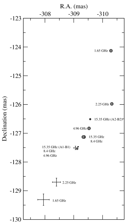
Figure 7: The A and B peak–to–peak separation (plus symbols) as a function of frequency. At 15.35 GHz, separations for both the components A1$-$B1 and A2$-$B2 are marked. The A and B centroid–to–centroid separation is also shown (in circles) but the error bars are omitted for the sake of clarity.

An advantage of imaging gravitational lenses is that any frequency–dependent position in the source can be seen as a frequency–dependence of the separation vector of the lensed images, without requiring the use of an external reference source. As mentioned in Section 1, this method is insensitive in cases where the position shift is along the same direction in both the images, but the accuracy of the measurement of the A$-$B separation is much higher than for that between B0218+357 and B0215+364. The peak–to–peak image separations at different frequencies, measured with MAXFIT in full resolution maps, are shown in Figure 7. Since the images at 15.35 GHz are resolved into sub–components 1 and 2, the separations of both A1$-$B1 and A2$-$B2 are indicated in the plot. We see that the separation at 15.35 GHz (A1$-$B1), 8.4 GHz and 4.96 GHz remains roughly the same, implying that the “peak” is centred around component 1 in both the images. At 2.25 GHz and 1.65 GHz, the separation increases in declination and decreases in right ascension, in a direction opposite to component 2. This is surprising as one might expect the separation at lower frequencies to gradually coincide with the A2$-$B2 separation, reflecting relatively more prominent emission from component 2 at the base of the jet. Shown in the same figure as circles are the centroid–to–centroid image separations which are inconsitent with the peak–to–peak separations, although the behaviour of the latter is in concert with the image–structures seen at low frequencies (see below).

At 1.65 GHz we identify another component in image A, separated by $\sim$ 10 mas from component 1 and $\sim-33\,^{\circ}$ P.A., shown in Figure 8. The origin of this newly–identified feature (hereon component 3) is of great interest and we have investigated how this can be part of the background source. On applying the lens model by Wucknitz et al. (2004), we deduce that in image B it should be $\sim$ 3 mas from component 1 as indicated in Figure 8. Unfortunately the resolution at this frequency is not enough ($\sim$ 7 mas) to resolve this separation. This can be seen by placing a component at the expected position of component 3 in image B, of strength equal to the peak intensity of component 3 in image A [Figure 8] divided by the relative magnification ratio at this position. On convolving this with the restoring beam, its effect can be assessed by comparing a slice made through it and the components 1 & 2 with the slice made through the same points in the observed image. As shown in Figure 8, including another component in image B analogous to component 3 in image A has no observable effect other than changing the centroid of the brightness distribution by distance less than the positional uncertainity. Therefore, we cannot distinguish whether component 3 is a distinct feature in the background source imaged in A by the smooth macro potential of the lens, or whether it is caused by some other mechanism. The shift in the centroid position of image A at 1.6 GHz can be attributed to the existence of component 3.

Figure 8: a) Second maximum (component 3) detected at 1.65 GHz in image A at a separation of $\sim 10$ mas from component 1 & 2 (The components 1 and 2 are not resolvable at these frequencies, hence what is marked is their superposition). b) The predicted position of component 3 in image B at 1.65 GHz, marked as a black dot about $\sim$ 3 mas from component 1 & 2. The resolution at this frequency is about 7 mas. c) A slice through the components 1 & 2 and 3 in image A. d) The predicted and observed slices through the components 1 & 2 and the expected position of component 3 in image B.

6 Discussion

We have successfully used the technique of inverse phase–referencing to investigate the frequency–dependence of the emission from the images of B0218+357; we believe this is the first time in which a gravitational lens has been used as a phase–reference. We have established the change in the centroid position of the image brightness distributions over five frequencies, and also investigated the change in the positions of the emission peaks using inter–image astrometry. The shift in the centroid in image A, which is significant ($\sim$ 5 mas) only at 1.65 GHz, is in a direction along which the relative magnification is predicted to be constant. In image B no significant frequency dependent shift is detected in the position of the centroid. A reasonable assumption is that the relative image magnification at the centroid positions derived from the model gives a good measure of the expected image flux–density ratio. Thus we conclude that the changing magnification gradient across the images is not the main cause of the anomalous change of image flux–density ratio with frequency.

As can be clearly seen in Figure 3, at 1.65 GHz there is a large amount of low brightness emission that extends out to $\sim\pm$ 30 mas. In comparison, at 15.35 GHz the emission is dominated by the compact sub–components with a separation of $\sim$ 1.4 mas. At lower frequencies the (larger) images extend over regions where lens models do, indeed, predict significant changes in the relative magnification, and it may be insufficient to simply consider magnifications at the centroid positions. This is because low frequency emission from different regions of the background source is magnified by very different amounts. The resultant average magnification is thus the integral of the (background source) intensity–weighted magnification over the image area.

We plan to extend our study by applying the model from LensClean and evaluating the ratio of the (background source) intensity–weighted magnifications of image A to B, explicitly taking the observed extension of the background source into account. We also want to extend our choice of lens model to one with a non–isothermal mass–radius profile. The motivation for this is the observation by Biggs et al. (2003) related to the jet stretching factor, which seems to be larger in image B than A, as seen when projected back to the source plane. But the deviation from non–isothermality is expected to be small (Wucknitz et al. 2004) since low–resolution VLA observations of the Einstein ring are fitted quite well with isothermal models.

The identification of a distinct secondary maximum in image A at low frequencies (component 3), the sharp downturn in the spectrum of image A at 1.6 GHz (not visible in image B) and the small shift in the 1.6 GHz peak position in A are further results from these observations with no obvious explanation in terms of the expected magnification gradients across the images. It may, therefore, be necessary to consider more elaborate mechanisms, such as mass sub–structure (milli–lensing), free–free absorption or refractive scattering in the lens galaxy, to account for all the observed features in the B0218+357 images. Milli–lensing can produce significant frequency–dependent changes in the flux–density of one (or both) of the images provided the source size is comparable to the Einstein radius of the perturber and changes appreciably with frequency relative to it. The source size changes by a factor 30 over the observed frequency range and its interaction with the caustics of the perturber can bring about frequency–dependent changes in the total magnification (Dobler & Keeton 2005). Non–gravitational effects such as free–free absorption or scattering will cause flux–density perturbations that follow an inverse frequency power–law. The effects produced by the above mechanisms on the image flux–density ratio in B0218+357 are a subject in their own right and are beyond the scope of the present article (Mittal 2006, in preparation).