Chemistry and Star Formation in the Host Galaxies
of Type Ia Supernovae

Abstract

We study the effect of environment on the properties of type Ia supernovae by analyzing the integrated spectra of 57 local type Ia supernova host galaxies. We deduce from the spectra the metallicity, current star formation rate, and star formation history of the host and compare these to the supernova decline rates. Additionally, we compare the host properties to the difference between the derived supernova distance and the distance determined from the best-fit Hubble law. From this we investigate possible uncorrected systematic effects inherent in the calibration of type Ia supernova luminosities using light curve fitting techniques. Our results indicate a statistically insignificant correlation in the direction higher metallicity spiral galaxies host fainter type Ia supernovae. However, we present qualitative evidence suggesting progenitor age is more likely to be the source of variability in supernova peak luminosities than is metallicity. We do not find a correlation between the supernova decline rate and host galaxy absolute B magnitude, nor do we find evidence of a significant relationship between decline rate and current host galaxy star formation rate. A tenuous correlation is observed between the supernova Hubble residuals and host galaxy metallicities. Further host galaxy observations will be needed to refine the significance of this result. Finally, we characterize the environmental property distributions for type Ia supernova host galaxies through a comparison with two larger, more general galaxy distributions using Kolmogorov-Smirnov tests. The results show the host galaxy metallicity distribution to be similar to the metallicity distributions of the galaxies of the NFGS and SDSS. Significant differences are observed between the SN Ia distributions of absolute B magnitude and star formation histories and the corresponding distributions of galaxies in the NFGS and SDSS. Among these is an abrupt upper limit observed in the distribution of star formation histories of the host galaxy sample suggesting a type Ia supernovae characteristic delay time lower limit of approximately 2.0 Gyrs. Other distribution discrepancies are investigated and the effect on the supernova properties are discussed.

1 Introduction

Among the powerful tools that have come into prominence in the last decade in the field of cosmology, few have been as important in advancing the subject as type Ia supernovae (SNe Ia). SNe Ia show variations in their peak luminosities and colors that correlate well with their light curve decay times (Phillips, 1993; Hamuy et al., 1996c; Reiss, Press, & Kirshner, 1996; Perlmutter et al., 1999) making SNe Ia the best distance indicators. Application of this empirical relationship to the low-z sample of galaxies enabled cosmologists to refine the measurement of the Hubble Constant with great precision (Jha et al., 1999; Freedman et al., 2001).

Realizing the potential for SNe Ia to act as accurate cosmological probes, researchers applied the technique to the high-z sample of galaxies (Perlmutter et al., 1997; Garnavich et al., 1998; Schmidt et al., 1998). This research has yielded evidence suggesting that our universe is in a state of accelerating expansion implying a form of dark energy whose nature we do not yet understand (Riess et al., 1998; Perlmutter et al., 1999). The goal of the ESSENCE project is to improve our understanding of this negative pressure by placing tight constraints on the cosmic equation of state through a study of $\sim$200 SNe Ia at intermediate redshifts. The result will be a detailed map of the history of cosmic expansion with less than 2% distance error in six redshift bins and the ability to constrain the equation of state to 10%. Moreover, future studies will attempt to differentiate between a vacuum energy and other more exotic sources for the acceleration (Wang & Garnavich, 2001; Miknaitis et al., 2005) that will push the limits of the SNe Ia reliability. Clearly, it is of paramount importance to understand any systematic uncertainties in the calibration of SNe Ia that could bias these cosmological measurements.

Type Ia supernovae are identified by the presence of singly ionized silicon, magnesium, sulfur, calcium, and the conspicuous absence of hydrogen in their spectra. Early statistical studies of type I supernovae and their host galaxies showed that the events, like core-collapse SNe, are associated with young stellar populations (Oemler & Tinsley, 1979; Caldwell & Oemler, 1981). However, unlike their core-collapse counterparts, type Ia supernovae are readily observed far from the spiral arms in spiral galaxies and in early-type galaxies with low star-formation rates. These observations require a delay between formation and explosion that is long enough to allow for proper diffusion away from the spiral arms (McMillan & Ciardullo, 1996) and imply a lower mass for the SNe Ia progenitors. Specifically, SNe Ia are thought to be triggered by thermonuclear ignition in the core of a CO white dwarf near the Chandrasekhar mass limit (1.4 M_☉). Two models predict how the WD attains the mass necessary to initiate explosive burning. The first model is the single degenerate model (Whelan & Iben, 1973; Nomoto, 1982) that describes a binary system in which a WD accretes matter from a main sequence or red giant binary companion. The second model, the double degenerate model (Webbink, 1984; Iben & Tutukov, 1984), describes the coalescing of two binary WDs whose combined mass exceeds the Chandrasekhar mass limit. Once the mass limit is reached, carbon ignites resulting in the outward propagation of a burning front from the WD core.

Detonation occurs if the burning front travels outward faster than the local sound speed, but such an explosion would convert most of the star to nickel and would leave too few intermediate mass elements compared to the observed spectra. A deflagration results when the flame front traverses the star subsonically, but this tends to produce too little kinetic energy to account for the observed velocities. A combination of these two scenarios, known as the delayed detonation model (DD model) (Khokhlov, 1991; Yamaoka et al., 1992; Woosely & Weaver, 1994a) appears to best fit the observations. The DD model assumes flame front propagation velocity that begins as deflagration and subsequently transitions into detonation at a specific transition density. Although the DD model has been able to match many of the features observed in SNe Ia, there remains many open questions. For example, what triggers the transition to a detonation and how does the WD build mass to reach the Chandrasekhar limit?

These uncertainties reinforce the need to investigate systematic effects that can influence the luminosity-decline rate relation. One important effect is the possible evolutionary changes undergone by the stellar populations producing the supernova progenitors. For example, systematic differences between the high-z host stellar populations and the local host stellar populations could contribute to an inherent difference between the peak luminosities of low-z events and those of the high-z events. Fortunately, the local sample of galaxies provides such a wide range of host stellar environments that a study of these local environments can provide insight into environmental parameters that may correlate with redshift.

Theoretical models have shown that parameters such as progenitor mass and metallicity can have an effect on the luminosity and light curve shape of the resultant supernova by influencing the relative CNO abundances in the white dwarf. For the DD model, massive progenitors produce faint type Ia supernovae because of a low carbon fraction in the core (Höflich et al., 1998; Umeda et al., 1999). The carbon fraction is also lowered as the progenitor metallicity is increased resulting in less energetic explosions. For the range of masses expected for CO white dwarfs, lowering the carbon fraction is expected to affect the peak brightness of type Ia events by about 20%. The range in peak brightness due to progenitor metallicity variations is expected to be small unless the metal abundance is significantly higher than solar (Timmes, Brown, & Truran, 2003).

In order for predictions such as these to be tested observationally, it would be necessary to analyze a large sample of Type Ia supernova host stellar populations covering a wide range of ages and metallicities against the parameters of the supernovae they produce. Unfortunately, it is difficult to isolate and observe the specific stellar populations harboring the progenitor systems. Moreover, a long delay between formation and explosion would blur the correlation between a SN characteristics and its present local environment. Consequently, the majority of observational research in this topic has centered on the study of the integrated light from the SN Ia host galaxies. An analysis of the integrated light has the added advantage of allowing for future comparisons with high-z host galaxies whose small angular size restrict the observations to integrated spectra.

We characterize the SN environments through the spectroscopic study of 57 type Ia supernova host galaxies. We have two goals for this study. The first is to take a direct look at the possible systematic effects that the host galaxy environment has on the SN Ia properties through an analysis of the interdependencies between host galaxy and SN Ia parameters. Secondly, we take an indirect look at these systematics by comparing our SN host sample with two larger, more general samples of galaxies - the galaxies of the Near Field Galaxy Survey and those of the Sloan Digital Sky Survey. In §2 we introduce the host galaxy sample, detail the observing strategy, and present the data reduction process. In §3, the spectroscopic results are presented, and the theoretical predictions are discussed in light of the results. Finally, we summarize our conclusions.

2 Observations and Data Reduction

2.1 Observations

The host galaxy spectra reported here were obtained with the FAST spectrograph (Fabricant et al., 1998) at the F.L. Whipple Observatory’s 1.5 m Tillinghast telescope atop Mt. Hopkins in Arizona. The data were taken during 13 nights between 1999 May through 2000 September. The seeing ranged from 1″ to 2″ throughout the survey. The FAST spectrograph, with a 300 line mm^-1 reflection grating, allowed for 4,000 Å coverage and a FWHM resolution of $\sim$6 Å. The slit was 3″ wide and had an unvignetted length of 3′.

The slit was aligned along each host galaxy’s major axis to maximize the galactic light sampled. The position angles for each major axis was determined using the Digital Sky Survey Plates (DSS). The slit was offset to a distance matching the visible limit of the galaxy’s minor axis on the DSS and the slit was scanned repeatedly across the galaxy during an exposure. Exposure times ranged from 300 to 1,200 s depending on the brightness of the target. Seven of the target galaxies (NGC 2841, NGC 3368, NGC 3627, NGC 4526, NGC 4527, NGC 4536, and NGC 5005) had major axes that subtended angles larger than 3′. In these cases, we oriented the slit along the galaxy’s minor axis and scanned along its major axis. It should be noted that light losses due to atmospheric refraction are expected to be minimal given our use of a relatively wide 3″ slit and the fact that this slit was scanned across the entire visual extent of our galaxies, an extent that typically measured many times the width of our slit.

At the beginning and the end of each night’s run, both 12 s flat exposures and bias exposures were taken. Sky flats were taken to normalize the sensitivity along the slit. Flux standard star exposures were obtained twice per night with the slit oriented along the star’s parallactic angle (Filippenko, 1982). The standards were taken from the list given in Massey et al. (1988). Preceding the observation of every object galaxy, we obtained a comparison spectrum of a He-Ne-Ar lamp for reference in the wavelength calibration. For every object galaxy, save a few that will be addressed later, three images were taken with identical exposure times. Table 1 details our galaxy sample and the relevant observational parameters pertaining to each. Columns (1) and (2) give the common name of the target galaxy and the name of the supernova that it hosted, respectively. Column (3) shows the position angle of the slit for each object while the scan width is recorded in column (4). Column (5) gives the angular width of the extracted aperture for each host galaxy chosen to enclose all of the galactic light.

2.2 Data Reduction

The data reduction performed during this study was conducted following the standard techniques within the IRAF environment. The data were both dark and bias subtracted. Each galaxy spectrum was flat-fielded to correct for pixel-to-pixel variability in the CCD detector. Several pixels in each image were bad due to flaws on the CCD chip and had to be removed by interpolation. This was accomplished using the FIXPIX routine in IRAF. The acquisition of three identical spectra for each target galaxy allowed us to remove the majority of our cosmic rays by combining our images using the median parameter in the IRAF routine IMCOMBINE. Any further anomalous pixels were removed individually using IMEDIT.

There were two conditions under which we were unable to remove cosmic rays in this fashion. Firstly, in a few cases time constraints or poor atmospheric conditions prevented the acquisition of 3 spectra for the given target galaxy. In these situations, the cosmic rays were removed individually from those spectra we did obtain, and the images were averaged using IMCOMBINE. Secondly, in order to determine whether those objects with three images could be combined successfully using the median parameter in IMCOMBINE, it was necessary to ensure both that the spatial axes of each spectrum were aligned, and that they each had comparable background levels. Both of these tasks were accomplished using the IMPLOT routine to plot the average of several cuts along each image’s respective spatial axis. If the spatial axes were misaligned, they were shifted using the IMSHIFT routine in IRAF. Occasionally, short term atmospheric variability resulted in evident variations observed in the continuum levels of the three image set. If it was discernible which image(s) was bad, then that image(s) was removed and cosmic ray removal proceeded as detailed above on the remaining spectra. On the other hand, if the anomalous image(s) was not evident, then the cosmic rays were removed individually from each image, aperture extraction was performed, and the extracted apertures were averaged using IMCOMBINE.

The next step was to extract a one-dimensional spectrum from each combined image using the APALL routine in IRAF. The apertures were fitted interactively within IRAF and chosen to span a region on the spatial axis that extended slightly into the sky portion of the image on either side of the galaxy spectrum. In this way we ensured the inclusion of nearly 100$\%$ of the galactic light. However, attempts were made to avoid the inclusion of foreground stars in the aperture. The sky levels and trace were defined interactively using APALL with a linear fit for the former and a third order cubic spline for the latter. Wavelength and flux calibration proceeded using the standard techniques within IRAF.

Following the flux calibration, a telluric absorption correction was performed on those galaxy spectra containing relevant emission lines (i.e. H$\alpha$ and SII) that have been redshifted into the B-band (6860-6890 Å ) and beyond. Next, the spectra were dereddened to account for local reddening due to Galactic extinction. This was done using the routine DEREDDEN in IRAF. In each case a value of 3.0 was taken for the total to selective visual absorption ratio, R. Furthermore, the value of the color excess, E(B-V), was chosen for each galaxy direction to correspond to that which is stated by the NASA/IPAC Extragalactic Database (NED). These color excess values were calculated from COBE, the IRAS maps, and the Leiden-Dwingeloo maps of HI emission. Finally, the galaxy spectra were Doppler corrected using the routine DOPCOR with redshifts obtained from NED.

2.3 Line Strengths

Following reduction the spectral properties were analyzed through the identification and subsequent line profiling of various relevant spectral lines. In each case the line strengths were recorded using the SPLOT routine within IRAF. Gaussian line profiles were fit for each emission line individually with the primary source of error originating in the continuum definition. If appropriate, a boxcar smoothing algorithm was applied interactively allowing for more accurate continuum definition. We obtained both equivalent width (EW) and line fluxes for [OII] $\lambda$3727 (our resolution was insufficient to resolve the [OII] doublet), H$\beta$ $\lambda$4861, [OIII] $\lambda$4959, [OIII] $\lambda$5007, [OI] $\lambda$6300, [NII] $\lambda$6548, H$\alpha$ $\lambda$6562, [NII] $\lambda$6584, [SII] $\lambda$6717, [SII] $\lambda$6731. The equivalent widths measured in Angstroms are shown in Table 2 while emission-line fluxes in units of 10^-14 ergs cm^-2 s^-1 are given in Table 3, respectively.

3 Results

3.1 Host Galaxy and Supernova Parameterization

Here we describe the parameters which characterize the galaxies in the SN Ia host sample. The galactic parameters are given in Table 4. Columns (3)-(6) are observed while columns (7) and (8) are derived parameters. Column (1) lists the galaxies in our sample while column (2) gives each galaxy’s hosted supernova. The absolute B magnitudes of each host along with their corresponding errors are recorded in columns (3) and (4), respectively. The vast majority of magnitudes were calculated from distances derived from their respective redshifts. In a few cases, the potential for uncertainty was heightened due to the low recessional velocity of the host galaxy. Therefore, other distance measurements from the literature were employed for these cases when possible. Cepheid based distance moduli were found for NGC 3368, NGC 3627, NGC 4639, and NGC 4536 from the HST Key Project published in Gibson et al. (2000). The distance to NGC 4526 was determined by Hamuy et al. (1996b) using the Surface brightness fluctuations/planetary nebula luminosity function and published in Hamuy et al. (2000) (hereafter H00). All magnitudes were corrected to correspond to a Hubble constant of 72 km s^-1 Mpc^-1. Column (5) lists the morphological types according to NED while column (6) shows the H$\alpha$ luminosity for each host galaxy.

The derived galactic parameters were metallicity and birthrate parameter b (Scalo, 1986). These are shown in columns (7) and (8), respectively. For those host galaxies with distinguishable emission lines, we determined the metallicities from our emission line flux measurements using the models detailed in Kewley & Dopita (2002). The paper provides a series of line strength diagnostic diagrams with various dependences on both metallicity and the local ionization parameter, q. One first estimates an initial metallicity through a diagnostic that varies little with q. The initial value is then used to pin down the value of the ionization parameter through a diagnostic with strong dependences on both metallicity and the ionization parameter. Successive iterations ultimately provide the best estimate of the galaxy’s metallicity. For full details see Kewley & Dopita (2002). Extinction correction was applied for those galaxies with measurable Balmer emission using the Whitford reddening curve as paramaterized by Miller & Mathews (1972). We were unsuccessful in obtaining metallicity estimates for galaxies with weak emission. Furthermore, our signal to noise was insufficient to provide accurate absorption line strengths needed for an absorption line metallicity estimate. However, three galaxies from our sample had metallicities measured in H00 that we used in our analysis.

The final host galaxy parameter was the Scalo b parameter (Scalo, 1986). The Scalo b parameter is the ratio of the current star formation rate to the average star formation rate of the past. The parameter was determined by interpolation of the plot given in Fig.3 from Kennicutt, Tamblyn, & Congdon (1994)(hereafter KTC94). The plot shows the dependence of b on EW(H$\alpha$ + [NII]) as dictated by the exponential plus burst model detailed in KTC94.

Our SNe were characterized according to the parameters shown in Table 5. Once again, Column (1) and (2) give the galaxy ID and SN name, respectively. Column (3) and column (4) give the decline rate parameter, $\Delta$m₁₅(B), and its corresponding error, respectively. $\Delta$m₁₅(B) is defined as the change in apparent magnitude from maximum to 15 days after maximum light in the supernova rest frame. It acts as a convenient, reddening free, indicator of luminosity. Finally, column (5) shows the Hubble residuals for the SN set. Assuming that type Ia supernovae are perfect standard candles, the extinction and light curve corrected absolute magnitudes for the SNe should be identical. The Hubble residual for an individual SN is then defined as the deviation of its light curve and color corrected absolute magnitude from the average light curve corrected magnitude in the SN set. Our magnitudes originate from the set of 80 Hubble flow SNe published in Jha (2002).

3.2 SNe Ia and Host Galaxy Correlations

It is the goal of this study to investigate the correlations between type Ia properties and their global host galaxy parameters. Some of these correlations have been explored observationally in the past. Hamuy et al. (1996b) reported that the most luminous SNe Ia tend to be hosted by late type, spiral galaxies. The same behavior is seen in Figure 1 where we have replicated the morphological classification versus decline rate plot of Hamuy et al. (1996b) for a large sample of host galaxies. The data was compiled from the SNe described in Phillips et al. (1999), Jha (2002), Riess et al. (1999), and Krisciunas et al. (2004). The vertical lines in Figure 1 represent the average decline rates for the SNe in late type and early type galaxies, respectively. They confirm the results of Hamuy et al. that the slower declining, more luminous supernovae are hosted by late type galaxies. However, it is important to note when grouping host galaxies by their morphological type that such a grouping does not necessarily imply the members of a common class possess similar physical characteristics such as metallicity and star formation histories. For example, Figure 1 highlights NGC 2841 and NGC 0632 which are categorized as Sa and S0 galaxies, respectively. However, NGC 2841 is a galaxy with none of the usual emission features typically observed in spiral galaxies. Moreover, NGC 0632, although tentatively labeled an S0 galaxy by NED, shows strong emission indicative of a starburst galaxy. This shows that the gross morphology provides a helpful, though incomplete picture of the host properties and that a more detailed host galaxy characterization is necessary.

3.2.1 Metallicity

Theoretical studies conducted by Höflich et al. (1998); Umeda et al. (1999); Höflich et al. (2000)(hereafter HNUW00) along with analytical analysis by Timmes, Brown, & Truran (2003)(hereafter TBT03) have suggested that the initial metallicity of the Ia progenitor can have a small, but possibly significant effect (particularly at high metallicity) on the luminosity of the resultant supernova. HNUW00 pointed out that the metallicity of the progenitor on the main sequence can affect the mass of the interior C/O core left behind as a WD, and ultimately affect the amount of ⁵⁶Ni produced in the explosion and the peak luminosity of the SN Ia. TBT03

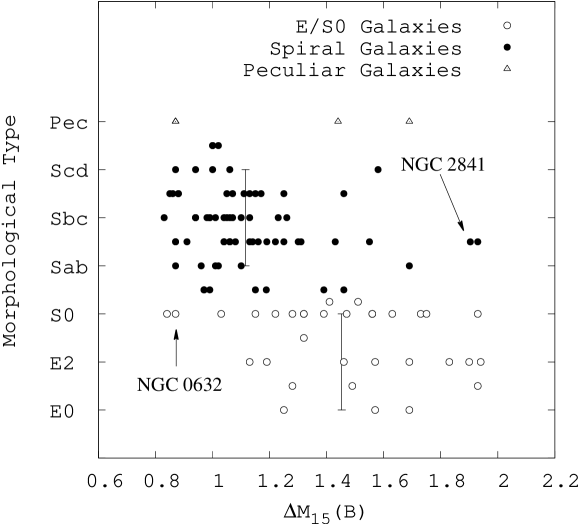
Figure 1: Morphological Type vs. Decline Rate of SN. Highlighted are NGC 2841, a categorized Sa galaxy with spectral features of an elliptical, and NGC 0632, a categorized S0 with the strong emission typically seen in late type galaxies. Vertical markers highlight the average decline rates for both early and late type host galaxies.

analytically demonstrated that a factor of three variation in progenitor metallicity results in an $\sim$25$\%$ variation is the mass of ⁵⁶Ni ejected during the Ia event. If one allows for the sedimentation of ²²Ne, then the variation can be as high as 50$\%$. Furthermore, Umeda et al. (1999) suggested that the carbon mass fraction in a CO white dwarf is dependent on the metallicity of the environment in which it was formed. They further proposed that the observed diversity in SNe Ia brightness is a consequence of this phenomenon with the smaller progenitor carbon fractions leading to dimmer supernova. Under the assumption that higher galactic metallicity is proportional to the average progenitor metallicity, we set out to investigate these theoretical results through observation.

Figure 2 shows the relationship between host galaxy metallicity and SNe Ia decline rate for our sample with a distinction drawn between elliptical and spiral galaxies. Two

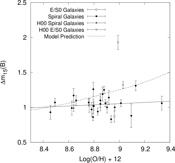
Figure 2: Decline Rate dependence on Metallicity. SN Ia sample of late types show a tendency for high metallicity galaxies to host fainter SNe Ia at the 70$\%$ confidence level. Addition of H00 galaxies further suggests a decrease in SN brightness with increased metallicity from early to late type galaxies. The solid line is a linear best fit to the data while the broken line represents the predicted trend governed by the studies of TBT03, Höflich et al. (2002), and Garnavich et al. (2004).

ellipticals and one spiral galaxy have been included with metallicities given in H00. A regression line is fitted to our host sample of spiral galaxies, and we find a small correlation suggesting that higher metallicity spiral host galaxies produce faster declining, less luminous SNe. However, a Monte Carlo simulation places this correlation at only the 70$\%$ confidence level. The simulation involved generating 25 evenly distributed metallicities between 8.3 and 9.4, assigning each one a $\Delta$m₁₅(B) from our data, and determining after a number of trials the probability of obtaining a best fit slope greater than or equal to the absolute value of the slope seen in Figure 2. This does not suggest that metallicity has a great affect on the luminosity of type Ia supernovae.

A comparison between the late type galaxies of H00 and our spiral galaxies at the same metallicity shows a wide dispersion in decline rate at a fixed metallicity likewise suggesting a weak dependence of Ia decline rate on the environment metallicity. However, the presence of two metal rich ellipticals from H00 that hosted SNe Ia with a higher decline rate on average than our spirals could hint at an overall increase in $\Delta$m₁₅(B) with metallicity across the full Hubble sequence. Such a trend would support the predictions made by the analytical models of TBT03. We use the DD numerical models of Höflich et al. (2002) and the empirical relations of Garnavich et al. (2004) to convert the predictions of TBT03 to the observed parameter. The predicted relation is shown in Figure 2 (broken line). Oxygen abundances were converted into iron abundances using the [O/Fe] to [Fe/H] relation predicted by the three-component mixing models of Qian & Wasserburg (2001). ⁵⁶Ni masses were calculated for the iron abundances according to the analytical model of TBT03. The decline rate lower limit in the plotted range is set by the M_Ni vs. metallicity relation presented in TBT03. We assumes a fiducial SN Ia M_Ni production of approximately 0.64M_☉. Varying this fiducial mass acts to vary the low metallicity decline rate limit. Interpolation of the M_V vs. M_Ni plot in Höflich et al. (2002) yielded corresponding M_V for each ⁵⁶Ni mass. Finally, we found corresponding decline rates through the empirical M_V vs. $\Delta$m₁₅(B) relation presented in Garnavich et al. (2004). This predicted curve is not meant to provide for a detailed comparison with the observations, but rather to convey the general metallicity-decline rate trend predicted by TBT03. The curve implies a minimal dependence of type Ia SN luminosity on metallicity for metallicities below solar. However, as progenitor metallicity increases well above solar, the predicted dependence becomes steeper resulting in significantly fainter SNe Ia.

Figure 3 shows the projected galactocentric distances (PGD) of type Ia supernovae versus $\Delta$m₁₅(B). The SNe were compiled from the list presented in Phillips et al. (1999), Jha (2002), Riess et al. (1999), and Krisciunas et al. (2004). Projected offsets were obtained from the Harvard CfA List of Supernovae and the Central Bureau for Astronomical Telegrams (CBAT). Hubble flow luminosity distances were calculated from the SN redshift assuming cosmological parameters H₀ = 72 km s^-1 Mpc^-1, $\Omega$_M = 0.28 and $\Omega$_Λ = 0.72 while non-Hubble flow distances were estimated using the SNe luminosities. A more even distribution in decline rates is observed for supernovae hosted by elliptical galaxies than those hosted by their smaller

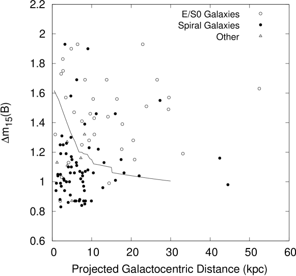
Figure 3: Type Ia supernovae decline rate versus projected galactocentric distance. Solid line represents the predicted decline in $\Delta$m₁₅(B) with PGD due to a decrease in metallicity with increasing PGD (Andrievsky et al., 2004).

spiral counterparts. The relevance of this plot to metallicity becomes clear when we compare it to the expected metallicity gradient across a typical spiral galaxy. Recent results by Andrievsky et al. (2004) have indicated that there is a drop of 0.6 dex in [Fe/H] across the disk of the Milky Way from approximately 4.0 kpc to 16 kpc. Assuming the Milky Way to be adequately representative of a typical spiral galaxy, we can find a theoretical relation between the SN PGD and its decline rate using the methods detailed above. The relation is potted in Figure 3, and it suggests that amongst SNe hosted by spiral galaxies, the fainter events are predicted to reside nearest the galactic center - a prediction that stands in contrast to the observations in Figure 3 showing the brighter events clustering at low PGDs.

We also compared the SN hosts with two larger sets of galaxies in the hopes of shedding light on possible systematic selection effects or, more interestingly, evolutionary effects present in the discovery of SNe Ia. The first set was the Near Field Galaxy Survey sample (NFGS). The NFGS is a collection of integrated and nuclear spectroscopy for approximately 200 galaxies in the near field. The sample was analyzed with the FAST spectrograph operating on the Tillinghast

Figure 4: Cumulative fraction plots for our SN host galaxy sample, NFGS galaxy sample, and the SDSS galaxy sample. KS-test finds the probability of the host galaxy distribution and the NFGS distribution being drawn from the same distribution to be 12.0$\%$. Moreover, we find that the likelihood of the host galaxy sample and the SDSS sample being drawn from identical galaxy distributions to be 94.5$\%$. Fig. 5. – The metallicity distributions for the SN host galaxy, NFGS, and SDSS samples.

telescope and includes galaxies of every morphological type covering 8 magnitudes in luminosity (Jansen et al., 2000)(Hereafter J00). We were able to calculate metallicities for 116 galaxies using the integrated emission line EW presented in J00. The second comparison distribution is a set of approximately 9,000 SDSS galaxies whose spectroscopic line strength data was obtained through the Carnegie Mellon University/University of Pittsburgh’s SDSS Value-Added Catalog (CMU-VAC). We were able to obtain 3,133 galaxy metallicities from the SDSS sample using the EW line strengths obtained from the CMU-VAC. For consistency, host galaxy metallicities used for comparison with the NFGS and the SDSS metallicity distributions were calculated from emission line EW ratios, and both the NFGS and SDSS samples were limited to emission line galaxies.

We performed a Kolmogorov-Smirnov test to determine the likelihood that our host galaxies were drawn from similar distributions as the NFGS sample and the SDSS sample. Figure 4 and Figure 5 show the cumulative fraction plots (CFP) and the histograms for the metallicity distributions in each sample, respectively. We find from a KS test that the observed SN host galaxies could be drawn from the NFGS sample (12.0$\%$ probability) or from the SDSS sample (94.5$\%$). The consistency between Ia host distribution, the NFGS distribution, and particularly the SDSS distributions implies a high probability that the SN hosts do not have a unique metallicity signature as compared to a general sample of field galaxies, suggesting that the probability of a SN Ia occuring is not strongly dependent on the metallicity of the host galaxy in the range 0.05Z_☉ $\lesssim$ Z $\lesssim$ 3.5Z_☉.

3.2.2 Age

In each of the Figures (2-5) the observed behaviors fall into one of two categories. They either show a negligible effect of metallicity on the luminosity of type Ia supernovae, or they show a trend that opposes current theoretical predictions. In either case, the results suggest that metallicity is unlikely to be the primary contributor to the variability observed in the peak luminosities of type Ia supernovae. Another property known to be correlated with host galaxy morphology is population age. The population age, which we use as an approximation of the progenitor age, may be able to explain the luminosity variations of SNe Ia and the correlation of these luminosities with host galaxy morphological type (Figure 1). The progenitor age is the amount of time between the birth of the progenitor and the time of the supernova event. We can investigate the effect of progenitor age on the SN Ia luminosity distribution using a simple model inspired by Umeda et al. (1999). This is shown in Figure 6. We first adopted the single degenerate Chandrasekhar mass model for our SN progenitor system. We then randomly selected pairs of stars, M₁ and M₂, from a distribution of stars consistent with the IMF in Kroupa et al. (1993). A constraint is placed on the secondary mass requiring:

$$(M_{2}-M_{WD_{2}})+M_{WD_{1}}\geq 1.4M_{\sun}$$ (1)

where M${}_{WD_{1}}$ and M${}_{WD_{2}}$ are the subsequent white dwarf masses corresponding to main sequence masses M₁ and M₂ (Dominguez et al., 1999). This ensured that the secondary possessed the necessary mass required for M${}_{WD_{1}}$ to attain the Chandrasekhar limit through mass accretion. To prevent the inclusion of stars that explode as core collapse SNe, we limited M₁ and M₂ to be $\leq$ 8M_☉. Finally, we assumed the SNe explosion occurs soon after the main sequence lifetime of the secondary, thus setting the progenitor age, i.e the delay time, by the lifetime of the secondary.

Figure 6a shows the distribution of progenitor age as a function of the M₁. For a given primary mass, there is an upper and lower limit placed on the mass of the secondary, and thus the lifetime of the secondary. The lower limit on the progenitor mass arises from the requirement that the secondary

Figure 6: The effect of progenitor age on the variations in type Ia supernova luminosity. Progenitor age as a function of primary mass is given in (a) assuming an IMF as published in Kroupa et al. (1993). The distribution of progenitor age with the predictions of Strolger et al. (2003) over-plotted (b). The SN Ia decline rate as a function of progenitor age (c), and the distribution of decline rates that results (d).

star have enough mass to put the M${}_{WD_{1}}$ over the Chandrasekhar limit. On the other hand, the upper limit arises from a need for the secondary to have a lower mass than the primary. Allowing the secondary to have a greater mass would simply exchange the respective labels of primary and secondary. Given the nature of stellar evolution, an upper limit on mass becomes a lower limit on age, and vice versa. The point where the two limits meet represents a system in which M₁ = M₂. Binning the age axis in Figure 6a yields the age distribution of SNe Ia in Figure 6b. We have over-plotted the derived distribution published in the results of Strolger et al. (2003) for the type Ia supernovae delay time, or the time between progenitor formation and the SN event. Our simple model is in good agreement with an average type Ia supernova delay time around 3 Gyrs.

Next, we set out to determine the expected effects that the progenitor age has on type Ia supernova decline rate by first approximating a linear fit to the plot of core mass versus main sequence mass from Dominguez et al. (1999) and converting our primary masses into white dwarf masses. Umeda et al. (1999) postulated that the M${}_{{}^{56}Ni}$, and consequently the brightness of the SN Ia, increases as the C/O ratio of the progenitor increases. Based on the postulate, they developed a model describing this dependency. Although the model should be treated with caution given that it is based on an unproven postulate, we use it in our toy model to merely provide a rough understanding on the effects of age on the decline rates of SNe Ia. Therefore, using these ⁵⁶Ni yields and the M${}_{{}^{56}Ni}$ to $\Delta$m₁₅(B) relations described in $\S$ 3.2.1, we converted the white dwarf masses to the expected SN decline rates. The resultant decline rate versus age scatter plot is shown in Figure 6c. By binning the $\Delta$m₁₅(B)

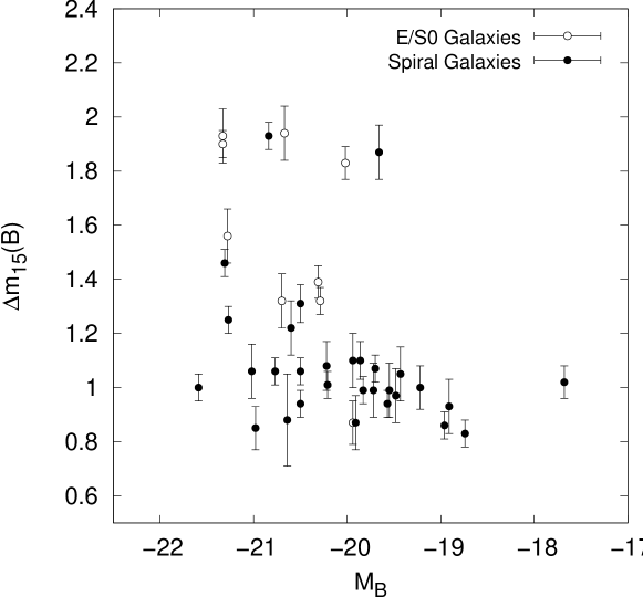
Figure 7: Decline rate versus Host Galaxy Absolute magnitude. Distribution shows an absence of dimmer SNe Ia in the low host galaxy luminosity regime.

axis we obtain the expected decline rate distribution for type Ia supernovae in Figure 6d. This figure shows that the age of the progenitor can result in a variation in decline rate similar to that which is observed for SNe Ia. This consistency is compelling evidence for age, not metallicity, acting as the primary source of SN Ia diversity. Future studies will obtain spectra of elliptical galaxies for use in absorption line metallicity and age estimations using the stellar population synthesis models of Worthey (1994). This will enable us to investigate the effects of age on the properties of type Ia supernovae directly.

3.2.3 Absolute B Magnitude

H00 showed, for a sample of nearby SN Ia host galaxies, a trend (with high dispersion) indicating that the SN Ia decline rate increases, and consequently its maximum luminosity decreases, with increased host galaxy luminosity. Henry & Worthey (1999) were able to show that the integrated luminosity of a galaxy is correlated with its global metallicity, as the brighter, more massive galaxies were able to better retain SN heavy metal ejecta. Therefore, H00 argued that any correlation observed between decline rate and absolute magnitude might manifest itself as a correlation between decline rate and metallicity. Figure 7 shows the absolute B magnitude of our host galaxy sample versus $\Delta$m₁₅(B). Although Figure 7 does not show the gradual trend observed by H00, the plot does show less scatter for the least luminous galaxies likely due to a combination of two effects. The first being a selection effect brought about by fewer SNe occurring in smaller galaxies. Such an effect would suggest that if we had more SNe from low luminosity galaxies, then the bias toward bright SNe Ia in the low galaxies luminosity regime would disappear. However, according to Figure 1, fainter SNe are predominantly hosted by elliptical galaxies which are on average brighter than spiral galaxies. Therefore, we see in Figure 7 a tendency for fainter SNe to be hosted by large, bright galaxies. The combination of these two effects contribute to the distribution observed in Figure 7.

Figure 8: Absolute magnitude distribution for the NFGS galaxy and Ia host galaxy samples. Histogram reveals the host galaxy distribution to be statistically brighter than the NFGS galaxy sample. Broken line is the theoretical SNe Ia distribution as predicted by our modified Schechter Function. Fig. 9. – Modified Schechter Function: Solid line shows the relative galactic luminosity, and consequently the galactic stellar population as a function of galaxy absolute B magnitude. The dot-dot-dash line shows the Schechter function as described by Schechter(1976). The modified Schechter function,dashed line, gives the relative probability of finding a type Ia SN as a function of galactic B filter magnitude.

Figure 8 shows the histograms of the NFGS and the SN Ia host galaxy distributions. The two distributions are clearly dissimilar owing to the nearly 2.5 magnitude discrepancy observed between the average magnitudes of the respective galaxy samples. The NFGS selected galaxies covering a wide range of luminosities (8 magnitudes), thus we would expect a broad distribution with little evidence of bias, as seen in Figure 8. On the other hand, the SN Ia host galaxy selection process was not subject to such regulations. However, several selection effects were ultimately present in the SN Ia search. Firstly, the selection of target galaxies in the supernova Ia search often involved point searches that focused on well known, and inevitably more luminous targets that would bias the SN host galaxies toward the higher luminosity regime. Furthermore, bias was introduced due to the non-uniformity of the Luminosity Function (LF) of galaxies. The form of the LF known as the Schechter function (Schechter, 1976),

$$\Phi(M)\sim 10^{-0.4(\alpha+1)M}e^{-10^{0.4(M^{*}-M)}}$$ (2)

with $\alpha$ = -1.17 and M^∗ = -20.73 given by the Century Survey (Geller et al., 1997), is plotted in Figure 9.

The LF illustrates that high luminosity galaxies are in the minority throughout the universe. Consequently, the probability of finding a SN Ia in a high luminosity galaxy is small, and the overall M_B distribution of SN Ia host galaxies will be shifted to the lower magnitudes. However, higher luminosity galaxies inherently have larger populations of stars than their lower luminosity counterparts. Figure 9 further reflects how the relative luminosity, and the stellar population of a galaxy changes with absolute B magnitude (function normalized to L${}_{(M_{B}=-18)}$ = 1). This curve assumes the luminosity in the B-band to be an adequate tracer of galactic mass. Although not the best tracer (Mannucci et al., 2005), in the absence of good near-infrared H or K band measurements, B-band should be sufficient for this analysis. We can see from the figure that although high luminosity galaxies are more rare than low luminosity galaxies, they possess more stars and thus have an increased probability of hosting a SN Ia. We can investigate the combined effects of these two phenomena through a Modified Schechter Function (MSF) represented by the product of these two functions governing the biases. This MSF, Figure 9, represents an approximate probability distribution governing the most likely absolute magnitudes for galaxies hosting SNe Ia. The MSF does a reasonable job in predicting the absolute magnitude distribution range for our set of SN Ia host galaxies (Figure 8).

3.2.4 Scalo Birthrate Parameter

H$\alpha$ equivalent width versus $\Delta$m₁₅(B) is given in Figure 10 while the H$\alpha$ luminosity is plotted against decline rate in Figure 11. The galaxies with no discernible H$\alpha$ emission are shown with their upper limits. They illustrate the propensity for the fastest declining type Ia SNe to occur in low emission galaxies. This result suggests that the current star formation is a galactic property at least partly responsible for the trend discovered by H00 and seen in Figure 1. Moreover, Figure 10 shows the H$\alpha$ distribution to be bimodal. The presence of a gap around an equivalent width of 18 Å suggests the possibility that there are two distinct populations of

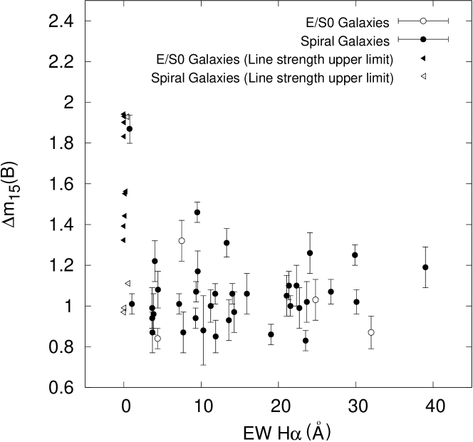
Figure 10: Supernova decline rate versus H$\alpha$ equivalent width. The gap present in the center of the distribution may suggest two distinct populations of type Ia supernovae.

type Ia supernovae. Scalo b is plotted against decline rate in Figure 12. Recalling the definition of Scalo b, we know that current star formation relative to that of the past increases with increasing b. Such a gap might suggest the existence of one type of SN with a short delay time residing in high star forming galaxies, and another type having a longer delay time residing in low star forming galaxies.

Figure 13 shows the cumulative fraction plots for the three distributions of Scalo b. Our goal was to compare the inherent differences between the galaxies of these three surveys; therefore, it was important to minimize the sample differences brought about by selection effects present in the design of each survey. One such selection effect apparent in the NFGS was that the quoted line strengths reported by J00 did not include specified upper limits. Such was not a reasonable expectation for the automated line fitting procedures used by SDSS. Consequently, weak line strengths that may not have been recorded in the NFGS would have been recorded by the SDSS. This would increase the relative populations of low star forming galaxies in the SDSS compared to the NFGS, and it would ultimately introduce uncertainty into our sample comparison. Therefore, we imposed a low end cutoff in the Ia host galaxy sample and the SDSS sample corresponding to the lowest Scalo b present in the NFGS. Although this prevented our ability to test the distributions among low star formation galaxies, it did ensure that the three distributions could be accurately compared at high Scalo b without the introduction of uncertainties due to inconsistent survey design at low Scalo b. The result of the KS-test reveal that the probability of the host galaxy distribution being drawn from the same distributions as the SDSS and the NFGS sample to be 3.2$\%$ and 0.9$\%$, respectively.

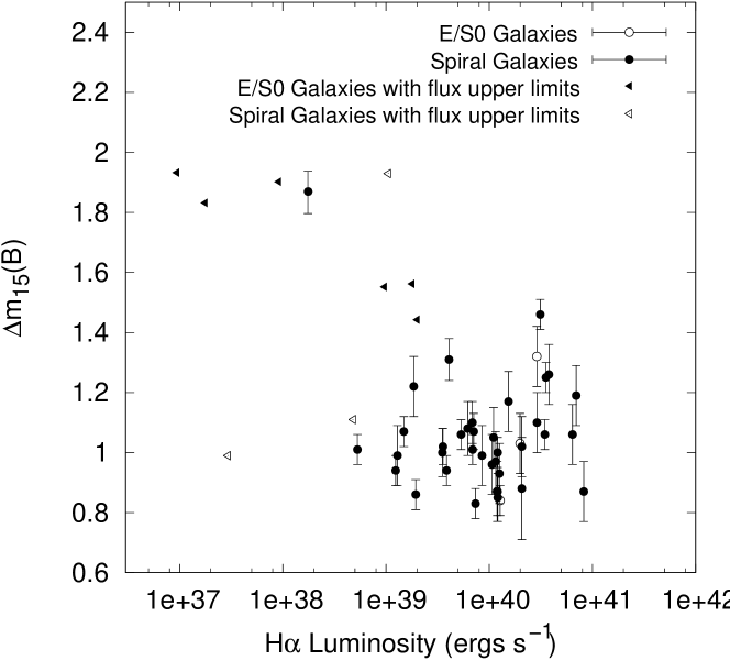
Figure 11: H$\alpha$ Luminosity versus $\Delta$m₁₅(B)

Qualitatively comparing the NFGS and SNe Ia host galaxy sample lead to the following differences. The aforementioned gap in H$\alpha$, and consequently Scalo b, along with a relative lack of low SFR galaxies in the NFGS result in the the SN Ia cumulative fraction plot increasing at a more rapid rate than the NFGS CFP. The second, and more intriguing difference is the lack of high SFR galaxies in the SN Ia host galaxy sample. Although similar at moderate Scalo b, the same disparity is seen between the Ia host sample and the SDSS sample at high Scalo b. Both the NFGS and the SDSS distribution turn over around b = 2.0, indicating the presence of high SFR galaxies in these respective samples. It is for this reason that the KS-test yields such low probability for the null hypothesis that the Ia distributions was drawn from the SDSS sample. This is also apparent in Figure 14 showing the Scalo b histograms for the three distributions.

The similarities observed between the SDSS sample and the Ia host sample at moderate Scalo b, combined with the intentionally non-partial nature of the NFGS suggest that the difference between the NFGS and the Ia host galaxy sample at low relative SFR does not suggest a meaningful discrepancy between Ia hosts and the general galaxy population. In reality, the difference is most likely a consequence of the NFGS selection process. KTC94 showed that Scalo b is correlated with galaxy morphological type. Consequently, we would expect a distribution of galaxies chosen to be uniform in morphological type and luminosity, such as the NFGS, to be likewise uniform in Scalo b.

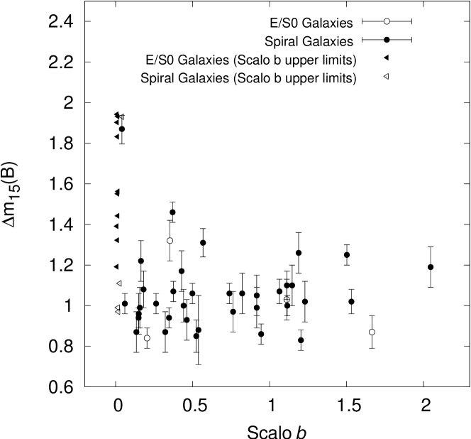
Figure 12: Scalo b parameter (Scalo, 1986) versus SN Ia light curve decline rate. Scalo b represents the current star formation relative to average past star formation.

However, the nature of the Ia host distribution at high Scalo b is inconsistent with that observed in both the NFGS and the SDSS galaxies samples. Galaxies with current star formation higher than approximately 2 times the average past SF seem to be selected out of the Ia host galaxy sample. A Monte Carlo test gives the probability of selecting 39 Scalo b values at random from the SDSS sample and fortuitously obtaining all values below 2.05 to be $\sim$0.05$\%$. Such a result implies a high significance for this cutoff.

A property of type Ia supernovae that has the potential to explain this rejection is the SN delay time, or alternately the time between progenitor formation and the supernova event. We investigated the implications of this cutoff given the following assumptions: 1.) The high star forming galaxies in the SN Ia sample have SFHs that are described by an exponential decline in SFR followed by a recent burst. We assume that the progenitor for each SN Ia hosted by a high star formation galaxy was thus formed during the current burst. 2.) There is a direct correlation between the number of SDSS galaxies observed in a particular Scalo b range (Figure 14) and the duration over which the average galaxy spends producing stars at that star formation rate (t_burst), and 3.) The ratio of the duration of a burst, with its peak at Scalo b = b^′, to the total lifetime of the galaxy ($\sim$ 14 Gyr) can be found through evaluation of the following:

$$Ratio = \frac{\int_{b^{\prime}}^{\infty}t_{burst}(b)db}{\int_{0}^{\infty}t_{burst}(b)db}$$ (3)

Given these three assumptions it is possible to place an approximate lower limit on the SN Ia delay time, $\tau$_min.

Figure 13: Cumulative fraction plots for our type Ia supernovae host galaxy sample, the NFGS sample of galaxies, and the SDSS galaxy sample. Fig. 14. — Scalo b distribution in the SN Ia host sample, the NFGS sample, and the SDSS sample. Note the cutoff in the SNe Ia host galaxy sample at b $\sim$ 2.

Our observed cutoff might suggests that galaxies with current star formation rates higher than b $\sim$ 2.0 are in the midst of a star formation burst that is too short to have created a SN Ia progenitor while allowing ample time for it to evolve and explode. By approximating an average galactic lifetime of 14 Gyrs, an evaluation of equ.(3) for b^′ = 2.0 results in a $\tau$_min $\sim$ 2.0 Gyrs. Recent work conducted by Gal-Yam & Maoz (2004) attempted to constrain $\tau$_min by comparing the theory and observation of the SN Ia redshift distribution. Beginning with theoretical functions governing the SFH and SN Ia delay time they calculated the expected redshift distribution of SNe Ia and compared this to the observed distribution of supernovae discovered by the Supernova Cosmology Project. The SFH function and SN Ia delay function are degenerate and thus could not be simultaneously constrained. A SFH function had to be assumed in order to constrain the SN Ia delay function, and vice versa. Assuming the SFH function predicted by Madau et al. (1998b), the results predict $\tau$_min = 1.7h^-1 Gyrs, $\sim$ 1.2 Gyrs, at the 95$\%$ confidence level. However, they go on to show that a longer characteristic delay time lower limit, $\tau$_min $\geq$ 3h^-1 Gyrs (2.1 Gyrs), is allowed if the SFH model of Lanzetta et al. (2002) is assumed.

3.3 Hubble Residual

Assuming a positive correlation between between galactic and progenitor metallicity, our results indicate that it is unlikely that variations in progenitor metallicity can entirely account for the large brightness variations observed in SNe Ia at peak luminosity. Although not a primary contributor, metallicity may contribute to more subtle variations at the level of the SN Ia intrinsic scatter. This can be tested by plotting the SN Hubble residuals, which are expected to have variations on the order of 0.18 mag (Jha, 2002), versus galactic metallicity (Figure 15a). The plot appears to show a slight trend for higher metallicity galaxies to produce SNe Ia with negative Hubble diagram residual.

Figure 15: Systematic errors present in the SN Hubble residuals. Figure shows the relationship between Hubble residual and host galaxy metallicity (a), host galaxy absolute magnitude (b), Scalo b (c), and the log of H$\alpha$ luminosity (d). A representative error bar is given in the lower left. Monte Carlo tests reveal the correlations to be statistically insignificant to varying degrees.

A Monte Carlo simulation reveals this correlation amplitude to be 90$\%$. The test was conducted as follows. We generated 16 Gaussian distributed random numbers using a standard deviation of 0.18 and assigned to each one a metallicity measurement from our data. We then plotted the metallicity versus this theoretical residual and calculated the slope of the best fit line. Repeated trials allowed us to determined the likelihood of obtaining a best fit slope to the data greater than or equal to the absolute value of the slope observed in the best fit to Figure 15a. This is a less than 2$\sigma$ detection and should be treated with caution. Although, it could suggest metallicity to be a secondary parameter affecting the brightness of SNe Ia at the 10$\%$ level. Nevertheless, continued study is need to bring about a more conclusive understanding. Figures 15(a-c) show similar plots for absolute magnitude, Scalo b, and the log of H$\alpha$ luminosity. We found insignificant correlations for these three parameters with Monte Carlo simulations placing the linear fits near the 75$\%$, 75$\%$, and 50$\%$ confidence levels, respectively.

3.4 Summary

We have analyzed the globally integrated spectra for a sample of type Ia supernova host galaxies in order to investigate the possible systematic effects that the host galaxy environment has on the properties of type Ia supernovae. We looked for direct correlations between the decline rates of type Ia supernovae and host galaxy metallicity, absolute B filter magnitude, and star formation rate. We further looked for correlations between these galactic parameters and the resident supernova’s Hubble best fit residual. Finally, we investigate the systematic differences between SN Ia host galaxies and the general galactic population through a series of Kolmogorov-Smirnov tests. The main results are as follows:

1. We find no correlation between spiral galaxy metallicity and SN Ia decline rate. We find significant decline rate variability at fixed host galaxy metallicity implying a small impact of metallicity on the peak luminosity of type Ia supernovae. We find that SNe at smaller PGDs have a higher average luminosity than those residing further from their galaxy’s nucleus. As metallicity is predicted to decrease as a function of PGD in spiral galaxies, this result stands on contrast to the predictions made by combining the results of TBT03, Höflich et al. (2002), and Garnavich et al. (2004). Furthermore, a KS-test shows the SN Ia host galaxy metallicity distribution to be statistically similar to the the NFGS, and particularly the SDSS metallicity distributions. Our results also indicate that the progenitor age can have a significant impact on the variations in type Ia decline rates. Assuming that the global galactic metallicity is approximately correlated with the progenitor metallicity, this implies that it is the age, and not the metallicity, of the progenitor that is the greater contributor to the inhomogeneities in type Ia supernovae explosions.

2. The gradual trend found by H00 between host galaxy absolute magnitude and supernova decline rate is not seen in our galaxy sample. Nevertheless, similar to the results of H00, we do find a lack of faint SNe in the low luminosity galaxy regime. This is most likely a combination of the expected lack of SNe in small galaxies and the behavior observed in Figure 1 that shows the tendency for low luminosity SNe Ia to be hosted almost exclusively by early type galaxies. Since ellipticals are on average brighter than other galaxies on the Hubble sequence, we would expect low luminosity SNe Ia to confine themselves to brighter host galaxies. The average absolute B magnitude of our host galaxies are found to be systematically brighter than the galaxies of the NFGS. The phenomenon can be attributed to the combined selection effect due to the increased population of stars in high luminosity galaxies and the non-uniformity of the luminosity function of galaxies.

3. We do not see evidence for a dependency of supernova decline rate on Scalo b in host galaxies with active star formation. However, we do see a discontinuity is the relationship between star formation rate and star formation history. To the extent that all of the fast declining SNe Ia studied have been hosted by galaxies with low, to non-existent, star formation. Moreover, the distribution of Scalo b for the host galaxy sample shows bimodal behavior suggesting the possibility of two distinct populations of type Ia supernovae possessing different delay times. The host galaxy Scalo b distribution also shows an unexpected cutoff at b $\sim$ 2 that might be indicative of a finite lower limit on the delay time of type Ia supernovae. We approximate this lower limit to be 2.0 Gyrs, slightly higher than the best value of 1.2 Gyrs obtained by Gal-Yam & Maoz (2004). Future refinements to the SFH models should help to finally pin down the true characteristic delay time.

4. Our tests to determine the effects of host galaxy environment on the SN Hubble residual all proved to be inconclusive to varying degrees. However, a 90% significance to a trend tying metallicity to Hubble residual, though requiring more study to prove or disprove, could suggest that metallicity, though not likely responsible for the diversity if SNe Ia brightnesses on the order of 1 magnitude, could be responsible for more subtle brightness variation seen at the 0.1 magnitude level. A continuation of this work currently underway is attempting to increase the host galaxy population used in this study which will enable us to improve the likelihood of detecting statistically significant results.

Table 1: The Host Galaxy Sample

Galaxy	SN	P.A.	Scan Width	Aperture Width
NGC 4536	1981B	30	120″	51″
NGC 3627	1989B	90	3′	71″
NGC 4639	1990N	-10	1′	51″
CGCG 111 016	1990O	-67	15″	23″
NGC 4527	1991T	-25	120″	46″
IC 4232	1991U	5	20″	31″
NGC 4374	1991bg	-50	3′	38″
Anon	1992J	85	15″	26″
IC 3690	1992P	-5	15″	18″
Anon	1992ag	100	15″	29″
Anon	1992bp	40	15″	17″
CGCG 307 023	1993ac	150	15″	18″
NGC 4526	1994D	20	90″	46″
NGC 4493	1994M	-20	20″	34″
CGCG 224 104	1994Q	70	10″	14″
NGC 4495	1994S	-45	20″	46″
NGC 3370	1994ae	-35	1′	23″
NGC 2962	1995D	-5	1′	46″
NGC 2441	1995E	-20	1′	51″
IC 1844	1995ak	100	15″	36″
NGC 3021	1995al	100	30″	46″
UGC 03151	1995bd	100	15″	51″
Anon	1996C	0	15″	23″
NGC 2935	1996Z	-30	2′	49″
Anon	1996ab	-30	0″	15″
NGC 5005	1996ai	-25	2′	51″
Anon	1996bl	80	15″	17″
NGC 0673	1996bo	0	45″	54″
UGC 03432	1996bv	130	15″	46″
NGC 2258	1997E	150	15″	29″
NGC 4680	1997bp	30	20″	40″
NGC 3147	1997bq	0	90″	68″
Anon	1997br	-20	20″	63″
NGC 5490	1997cn	10	20″	34″
NGC 0105	1997cw	0	30″	46″
UGC 03845	1997do	-10	30″	46″
NGC 5440	1998D	50	30″	23″
NGC 6627	1998V	80	15″	34″
NGC 4704	1998ab	45	30″	29″
NGC 3982	1998aq	90	1′	57″
NGC 6495	1998bp	20	20″	34″
NGC 3368	1998bu	45	2′	57″
NGC 0252	1998de	90	30″	40″
CGCG 302 013	1998di	$-$30	0″	17″
UGC 00139	1998dk	80	15″	51″
Anon	1998dm	20	15″	68″
Anon	1998dx	-30	10″	29″
UGC 03576	1998ec	130	30″	38″
UGC 00646	1998ef	100	15″	19″
NGC 0632	1998es	$-$20	$\cdots$	31″
CGCG 180 022	1999X	-20	15″	17″
NGC 2595	1999aa	-20	1′	57″
NGC 6063	1999ac	-30	30″	34″
NGC 2841	1999by	65	2′	51″
NGC 6038	1999cc	90	30″	50″
NGC 6411	1999da	70	20″	31″
NGC 6951	2000e	0	$\cdots$	32″

Table 2: Emission Line Equivalent Widths (Å)

Galaxy	SN	[OII]$\lambda$3727	H$\beta$$\lambda$4861	[OIII]$\lambda$4959	[OIII]$\lambda$5007	[OI]$\lambda$6300	[NII]$\lambda$6548	H$\alpha$$\lambda$6562	[NII]$\lambda$6584	[SII]$\lambda$6717	[SII]$\lambda$6731
NGC 4536	1981B	10.95	2.77	0.65	2.29	1.03	2.91	21.36	9.18	5.29	3.93
NGC 3627	1989B	1.27	1.74	0.10	0.40	0.34	1.73	13.30	6.27	2.46	2.06
NGC 4639	1990N	20.76	1.39	0.29	1.65	0.88	1.14	9.34	5.23	3.00	1.76
CGCG 111 016	1990O	4.84	0.00	0.00	0.13	0.49	0.41	3.85	3.56	0.87	1.45
NGC 4527	1991T	3.20	0.60	0.18	1.78	0.00	0.85	9.29	4.70	1.62	1.66
IC 4232	1991U	10.84	2.83	0.77	0.66	0.55	4.27	15.92	7.65	2.38	7.41
NGC 4374	1991bg	$\cdots$	$\cdots$	$\cdots$	$\cdots$	$\cdots$	0.00	0.04	0.44	$\cdots$	$\cdots$
Anon	1992J	$\cdots$	$\cdots$	$\cdots$	$\cdots$	$\cdots$	0.00	0.25	0.39	$\cdots$	$\cdots$
IC 3690	1992P	13.08	0.42	0.36	1.13	1.06	1.17	7.69	5.20	2.45	2.37
Anon	1992ag	42.14	9.17	3.87	13.52	0.99	7.30	39.01	12.95	12.98	6.03
Anon	1992bp	8.73	0.00	0.00	3.04	0.00	1.89	7.49	5.64	5.18	6.12
CGCG 307 023	1993ac	$\cdots$	$\cdots$	$\cdots$	$\cdots$	$\cdots$	$\cdots$	$\cdots$	$\cdots$	$\cdots$	$\cdots$
NGC 4526	1994D	$\cdots$	$\cdots$	$\cdots$	$\cdots$	$\cdots$	0.05	0.00	0.16	$\cdots$	$\cdots$
NGC 4493	1994M	$\cdots$	$\cdots$	$\cdots$	$\cdots$	$\cdots$	0.18	0.12	0.19	$\cdots$	$\cdots$
CGCG 224 104	1994Q	25.97	5.60	0.37	2.15	0.82	2.00	24.80	6.61	6.10	3.85
NGC 4495	1994S	20.37	4.37	1.22	3.93	0.73	2.09	22.33	10.01	4.42	5.88
NGC 3370	1994ae	16.04	3.59	0.66	0.72	0.00	2.20	19.04	7.28	4.66	3.06
NGC 2962	1995D	$\cdots$	$\cdots$	$\cdots$	$\cdots$	$\cdots$	0.13	0.08	0.40	$\cdots$	$\cdots$
NGC 2441	1995E	12.06	2.55	0.40	1.42	0.13	1.58	11.82	5.99	3.51	2.62
IC 1844	1995ak	17.56	3.98	0.43	1.81	0.60	2.39	24.07	9.18	6.57	4.42
NGC 3021	1995al	13.29	4.35	0.49	1.49	0.76	2.87	23.51	9.69	4.01	3.51
UGC 03151	1995bd	$\cdots$	$\cdots$	$\cdots$	$\cdots$	$\cdots$	0.78	4.36	4.78	$\cdots$	$\cdots$
Anon	1996C	17.18	2.37	0.00	1.46	0.80	4.38	14.27	7.75	5.54	3.57
NGC 2935	1996Z	$\cdots$	$\cdots$	$\cdots$	$\cdots$	$\cdots$	0.98	4.01	3.42	$\cdots$	$\cdots$
Anon	1996ab	$\cdots$	$\cdots$	$\cdots$	$\cdots$	$\cdots$	0.61	3.71	2.87	$\cdots$	$\cdots$
NGC 5005	1996ai	$\cdots$	$\cdots$	$\cdots$	$\cdots$	$\cdots$	0.89	3.66	3.57	$\cdots$	$\cdots$
Anon	1996bl	3.66	0.48	0.30	0.85	0.84	2.25	9.56	5.53	3.24	2.27
NGC 0673	1996bo	20.42	6.34	1.98	3.52	0.59	3.40	29.89	11.20	6.30	5.31
UGC 03432	1996bv	16.45	2.40	0.83	4.47	0.83	1.39	13.58	3.37	4.88	4.30
NGC 2258	1997E	$\cdots$	$\cdots$	$\cdots$	$\cdots$	$\cdots$	$\cdots$	$\cdots$	$\cdots$	$\cdots$	$\cdots$
NGC 4680	1997bp	7.13	3.81	0.10	1.48	0.21	2.52	21.55	9.43	4.37	3.32
NGC 3147	1997bq	$\cdots$	$\cdots$	$\cdots$	$\cdots$	$\cdots$	0.83	7.15	4.08	$\cdots$	$\cdots$
Anon	1997br	41.89	5.65	2.27	13.02	1.70	3.55	30.09	9.74	4.11	3.89
NGC 5490	1997cn	$\cdots$	$\cdots$	$\cdots$	$\cdots$	$\cdots$	0.03	0.03	0.03	$\cdots$	$\cdots$
NGC 0105	1997cw	17.21	3.79	2.11	5.67	0.75	3.74	23.67	9.71	5.15	4.08
UGC 03845	1997do	31.51	4.81	1.03	5.44	0.53	1.36	22.70	6.04	6.00	4.71
NGC 5440	1998D	$\cdots$	$\cdots$	$\cdots$	$\cdots$	$\cdots$	0.32	0.11	1.93	$\cdots$	$\cdots$
NGC 6627	1998V	7.25	2.58	0.20	3.86	0.42	2.73	14.03	9.03	2.85	2.20
NGC 4704	1998ab	11.00	2.93	0.23	0.70	0.27	2.67	10.29	7.54	4.98	1.38
NGC 3982	1998aq	17.40	5.47	0.91	3.32	0.65	3.30	27.44	11.15	5.81	3.98
NGC 6495	1998bp	$\cdots$	$\cdots$	$\cdots$	$\cdots$	$\cdots$	0.09	0.02	0.15	$\cdots$	$\cdots$
NGC 3368	1998bu	$\cdots$	$\cdots$	$\cdots$	$\cdots$	$\cdots$	0.64	1.04	1.92	$\cdots$	$\cdots$
NGC 0252	1998de	$\cdots$	$\cdots$	$\cdots$	$\cdots$	$\cdots$	0.28	0.45	1.79	$\cdots$	$\cdots$
CGCG 302 013	1998di	$\cdots$	$\cdots$	$\cdots$	$\cdots$	$\cdots$	0.31	0.31	0.31	$\cdots$	$\cdots$
UGC 00139	1998dk	13.07	4.59	0.62	2.48	0.67	1.86	21.06	7.18	5.45	3.91
UGCA 017	1998dm	30.67	5.43	2.42	9.19	0.83	1.38	26.79	5.32	6.92	4.60
UGC 11149	1998dx	$\cdots$	$\cdots$	$\cdots$	$\cdots$	$\cdots$	0.14	0.14	0.14	$\cdots$	$\cdots$
UGC 03576	1998ec	10.80	0.00	0.08	0.14	0.50	1.00	4.41	3.66	1.64	4.20
UGC 00646	1998ef	$\cdots$	$\cdots$	$\cdots$	$\cdots$	$\cdots$	0.08	0.00	0.87	$\cdots$	$\cdots$
NGC 0632	1998es	21.55	6.82	0.74	3.03	1.60	3.89	31.99	13.11	6.87	5.38
CGCG 180 022	1999X	$\cdots$	$\cdots$	$\cdots$	$\cdots$	$\cdots$	0.25	0.60	0.70	$\cdots$	$\cdots$
NGC 2595	1999aa	15.35	0.54	0.26	0.42	0.00	1.55	11.88	6.66	3.17	2.91
NGC 6063	1999ac	9.16	2.56	0.00	0.78	0.46	1.27	11.24	5.22	2.71	4.22
NGC 2841	1999by	$\cdots$	$\cdots$	$\cdots$	$\cdots$	$\cdots$	0.11	0.74	1.65	$\cdots$	$\cdots$
NGC 6038	1999cc	$\cdots$	$\cdots$	$\cdots$	$\cdots$	$\cdots$	1.53	9.50	4.54	$\cdots$	$\cdots$
NGC 6411	1999da	$\cdots$	$\cdots$	$\cdots$	$\cdots$	$\cdots$	0.02	0.00	0.06	$\cdots$	$\cdots$
NGC 6951	2000E	$\cdots$	$\cdots$	$\cdots$	$\cdots$	$\cdots$	1.26	3.68	2.84	$\cdots$	$\cdots$

Table 3: Emission Line Fluxes (10¹⁴ ergs cm^-2 s^-1)

Galaxy	SN	[OII]$\lambda$3727	H$\beta$$\lambda$4861	[OIII]$\lambda$4959	[OIII]$\lambda$5007	[OI]$\lambda$6300	[NII]$\lambda$6548	H$\alpha$$\lambda$6562	[NII]$\lambda$6584	[SII]$\lambda$6717	[SII]$\lambda$6731
NGC 4536	1981B	3.11	0.76	0.20	0.68	0.30	0.86	6.32	2.72	1.58	1.18
NGC 3627	1989B	1.22	2.14	0.14	0.52	0.38	1.97	15.10	7.14	2.81	2.35
NGC 4639	1990N	4.94	0.60	0.13	0.71	0.34	0.45	3.68	2.05	1.19	0.70
CGCG 111 016	1990O	0.37	0.00	0.00	0.02	0.06	0.06	0.52	0.47	0.11	0.18
NGC 4527	1991T	0.84	0.38	0.09	0.59	0.00	0.35	3.76	1.90	0.64	0.65
IC 4232	1991U	0.10	0.60	0.13	0.13	0.08	0.72	2.68	1.29	0.40	1.24
NGC 4374	1991bg	$\cdots$	$\cdots$	$\cdots$	$\cdots$	$\cdots$	$\cdots$	0.03	0.32	$\cdots$	$\cdots$
Anon	1992J	$\cdots$	$\cdots$	$\cdots$	$\cdots$	$\cdots$	$\cdots$	0.04	0.07	$\cdots$	$\cdots$
IC 3690	1992P	0.59	0.04	0.04	0.12	0.10	0.12	0.79	0.53	0.24	0.24
Anon	1992ag	2.98	1.14	0.54	1.71	0.11	0.87	4.70	1.60	1.64	0.74
Anon	1992bp	0.18	0.00	0.00	0.09	0.00	0.05	0.20	0.15	0.13	0.15
CGCG 307 023	1993ac	$\cdots$	$\cdots$	$\cdots$	$\cdots$	$\cdots$	$\cdots$	$\cdots$	$\cdots$	$\cdots$	$\cdots$
NGC 4526	1994D	$\cdots$	$\cdots$	$\cdots$	$\cdots$	$\cdots$	0.06	$\cdots$	0.20	$\cdots$	$\cdots$
NGC 4493	1994M	$\cdots$	$\cdots$	$\cdots$	$\cdots$	$\cdots$	0.03	0.16	0.03	$\cdots$	$\cdots$
CGCG 224 104	1994Q	0.84	0.27	0.02	0.12	0.04	0.09	1.09	0.29	0.27	0.17
NGC 4495	1994S	2.90	0.97	0.31	0.92	0.18	0.49	5.25	2.35	1.03	1.37
NGC 3370	1994ae	2.22	0.65	0.21	0.14	0.00	0.16	3.19	1.21	0.75	0.49
NGC 2962	1995D	$\cdots$	$\cdots$	$\cdots$	$\cdots$	$\cdots$	0.04	0.02	0.13	$\cdots$	$\cdots$
NGC 2441	1995E	1.47	0.44	0.08	0.26	0.02	0.25	1.88	0.95	0.54	0.40
IC 1844	1995ak	1.91	0.64	0.08	0.31	0.09	0.37	3.69	1.41	0.98	0.66
NGC 3021	1995al	3.79	1.93	0.24	0.69	0.31	1.19	9.76	4.02	1.64	1.44
UGC 03151	1995bd	$\cdots$	$\cdots$	$\cdots$	$\cdots$	$\cdots$	0.47	2.59	2.80	$\cdots$	$\cdots$
Anon	1996C	0.57	0.13	0.00	0.08	0.04	0.22	0.70	0.37	0.27	0.17
NGC 2935	1996Z	$\cdots$	$\cdots$	$\cdots$	$\cdots$	$\cdots$	0.29	1.17	0.98	$\cdots$	$\cdots$
Anon	1996ab	$\cdots$	$\cdots$	$\cdots$	$\cdots$	$\cdots$	0.04	0.22	0.16	$\cdots$	$\cdots$
NGC 5005	1996ai	$\cdots$	$\cdots$	$\cdots$	$\cdots$	$\cdots$	0.89	3.67	3.58	1.71	0.90
Anon	1996bl	0.16	0.03	0.02	0.06	0.05	0.14	0.58	0.34	0.18	0.13
NGC 0673	1996bo	3.93	1.46	0.51	0.89	0.12	0.70	6.13	2.29	1.26	1.06
UGC 03432	1996bv	2.32	0.40	0.16	0.75	0.12	0.21	2.11	0.53	0.73	0.65
NGC 2258	1997E	$\cdots$	$\cdots$	$\cdots$	$\cdots$	$\cdots$	$\cdots$	$\cdots$	$\cdots$	$\cdots$	$\cdots$
NGC 4680	1997bp	1.92	1.15	0.03	0.47	0.06	0.75	6.42	2.81	1.30	0.99
NGC 3147	1997bq	$\cdots$	$\cdots$	$\cdots$	$\cdots$	$\cdots$	0.43	3.66	2.07	$\cdots$	$\cdots$
Anon	1997br	3.13	0.89	0.48	2.24	0.24	0.41	3.51	1.15	0.62	0.60
NGC 5490	1997cn	$\cdots$	$\cdots$	$\cdots$	$\cdots$	$\cdots$	0.01	0.01	0.01	$\cdots$	$\cdots$
NGC 0105	1997cw	2.52	0.72	0.43	1.09	0.12	0.60	3.82	1.56	0.81	0.63
UGC 03845	1997do	4.79	0.93	0.23	1.11	0.09	0.22	3.68	0.98	0.95	0.74
NGC 5440	1998D	$\cdots$	$\cdots$	$\cdots$	$\cdots$	$\cdots$	0.11	0.04	0.64	$\cdots$	$\cdots$
NGC 6627	1998V	1.65	0.92	0.08	1.46	0.16	1.07	5.51	3.55	1.12	0.87
NGC 4704	1998ab	0.62	0.34	0.03	0.09	0.03	0.32	1.23	0.88	0.62	0.17
NGC 3982	1998aq	5.93	2.53	0.46	1.64	0.26	1.33	11.10	4.46	2.29	1.57
NGC 6495	1998bp	$\cdots$	$\cdots$	$\cdots$	$\cdots$	$\cdots$	0.04	0.01	0.06	$\cdots$	$\cdots$
NGC 3368	1998bu	$\cdots$	$\cdots$	$\cdots$	$\cdots$	$\cdots$	0.84	1.37	2.52	$\cdots$	$\cdots$
NGC 0252	1998de	$\cdots$	$\cdots$	$\cdots$	$\cdots$	$\cdots$	0.13	0.20	0.80	$\cdots$	$\cdots$
CGCG 302 013	1998di	$\cdots$	$\cdots$	$\cdots$	$\cdots$	$\cdots$	0.01	0.01	0.01	$\cdots$	$\cdots$
UGC 00139	1998dk	2.34	0.85	0.21	0.50	0.17	0.32	3.59	1.22	0.92	0.66
UGCA 017	1998dm	9.28	1.89	0.97	3.46	0.25	0.41	7.84	1.55	1.98	1.31
UGC 11149	1998dx	$\cdots$	$\cdots$	$\cdots$	$\cdots$	$\cdots$	0.01	0.01	0.01	$\cdots$	$\cdots$
UGC 03576	1998ec	0.89	0.00	0.01	0.02	0.08	0.16	0.71	0.59	0.26	0.64
UGC 00646	1998ef	$\cdots$	$\cdots$	$\cdots$	$\cdots$	$\cdots$	0.02	0.00	0.22	$\cdots$	$\cdots$
NGC 0632	1998es	3.14	1.53	0.19	0.71	0.30	0.76	6.20	2.53	1.29	1.01
CGCG 180 022	1999X	$\cdots$	$\cdots$	$\cdots$	$\cdots$	$\cdots$	0.01	0.03	0.03	$\cdots$	$\cdots$
NGC 2595	1999aa	2.05	0.14	0.07	0.10	0.00	0.37	2.73	1.48	0.73	0.67
NGC 6063	1999ac	1.30	0.42	0.00	0.14	0.07	0.20	1.73	0.80	0.41	0.64
NGC 2841	1999by	$\cdots$	$\cdots$	$\cdots$	$\cdots$	$\cdots$	0.09	0.56	1.25	$\cdots$	$\cdots$
NGC 6038	1999cc	$\cdots$	$\cdots$	$\cdots$	$\cdots$	$\cdots$	0.23	1.44	0.70	$\cdots$	$\cdots$
NGC 6411	1999da	$\cdots$	$\cdots$	$\cdots$	$\cdots$	$\cdots$	0.01	0.00	0.03	$\cdots$	$\cdots$
NGC 6951	2000E	$\cdots$	$\cdots$	$\cdots$	$\cdots$	$\cdots$	0.91	2.63	2.00	$\cdots$	$\cdots$

Table 4: Galaxy Characterization

Galaxy	SN	MB	$\delta$MB	Morph. Type	H$\alpha$ Lum.	Log(O/H) + 12	Scalo b
		(mag)	(mag)		(ergs s-1)
NGC 4536	1981B	$-$19.86	0.11	Sbc	6.87E+39	8.66	1.11
NGC 3627	1989B	$-$20.5	0.24	Sb	4.08E+39	9.13	0.57
NGC 4639	1990N	$-$19.7	0.23	Sbc	1.49E+39	8.76	0.37
CGCG 111 016	1990O	$\cdots$	$\cdots$	Sba	1.07E+40	$\cdots$	0.15
NGC 4527	1991T	$-$20.5	0.27	Sbc	3.87E+39	8.83	0.35
IC 4232	1991U	$-$21.02	0.32	Sbc	6.42E+40	9.34	0.82
NGC 4374	1991bg	$-$21.33	0.07	E1	9.42E+36	$\cdots$	0.01
Anon	1992J	$-$21.28	0.14	S0$+$	1.79E+39	$\cdots$	0.01
IC 3690	1992P	$-$19.91	0.27	Sb	1.20E+40	$\cdots$	0.32
Anon	1992ag	$\cdots$	$\cdots$	S	6.97E+40	8.87	2.05
Anon	1992bp	$-$20.7	0.12	E2/S0	2.89E+40	$\cdots$	0.35
CGCG 307 023	1993ac	$\cdots$	$\cdots$	E	$\cdots$	$\cdots$	0.01
NGC 4526	1994D	$-$20.29	0.10	S0	$\cdots$	$\cdots$	0.01
NGC 4493	1994M	$\cdots$	$\cdots$	E+ pec	2.01E+39	$\cdots$	0.01
CGCG 224 104	1994Q	$\cdots$	$\cdots$	S0	1.99E+40	8.76	1.11
NGC 4495	1994S	$-$19.94	0.30	Sab	2.90E+40	8.85	1.15
NGC 3370	1994ae	$-$18.96	0.28	Sc	1.94E+39	8.79	0.95
NGC 2962	1995D	$-$19.83	0.28	Sa	2.94E+37	$\cdots$	0.01
NGC 2441	1995E	$-$20.77	0.28	Sb	5.34E+39	8.89	0.50
IC 1844	1995ak	$\cdots$	$\cdots$	Sbc	3.79E+40	8.79	1.19
NGC 3021	1995al	$-$18.74	0.30	Sbc	7.36E+39	8.94	1.20
UGC 03151	1995bd	$\cdots$	$\cdots$	S0	1.27E+40	$\cdots$	0.20
Anon	1996C	$\cdots$	$\cdots$	Sa	1.16E+40	8.78	0.76
NGC 2935	1996Z	$-$20.6	0.29	Sb	1.86E+39	$\cdots$	0.17
Anon	1996ab	$\cdots$	$\cdots$	$\cdots$	8.24E+40	$\cdots$	0.14
NGC 5005	1996ai	$-$19.72	0.29	Sbc	1.29E+39	$\cdots$	0.16
Anon	1996bl	$\cdots$	$\cdots$	SBc	1.54E+40	8.64	0.43
NGC 0673	1996bo	$-$21.27	0.31	Sc	3.55E+40	8.88	1.50
UGC 03432	1996bv	$-$18.91	0.31	Scd	1.26E+40	8.46	0.46
NGC 2258	1997E	$-$20.31	0.29	S0	$\cdots$	$\cdots$	0.01
NGC 4680	1997bp	$\cdots$	$\cdots$	Pec	1.21E+40	8.96	1.11
NGC 3147	1997bq	$-$21.59	0.28	Sbc	6.91E+39	$\cdots$	0.26
Anon	1997br	$-$17.68	0.32	Sbd	3.56E+39	8.80	1.53
NGC 5490	1997cn	$-$21.33	0.30	E	9.10E+37	$\cdots$	0.01
NGC 0105	1997cw	$\cdots$	$\cdots$	Sab	2.07E+40	8.79	1.23
UGC 03845	1997do	$-$19.55	0.30	SBbc	8.51E+39	8.62	0.92
NGC 5440	1998D	$-$20.35	0.31	Sa	1.36E+38	$\cdots$	0.04
NGC 6627	1998V	$-$20.5	0.39	Sb	3.46E+40	9.01	0.74
NGC 4704	1998ab	$-$20.64	0.31	Sbc pec	2.07E+40	9.09	0.54
NGC 3982	1998aq	$-$19.15	0.29	Sb	5.90E+39	8.92	1.41
NGC 6495	1998bp	$-$20.02	0.30	E	1.75E+37	$\cdots$	0.01
NGC 3368	1998bu	$-$20.21	0.22	Sab	5.28E+38	$\cdots$	0.06
NGC 0252	1998de	$-$20.84	0.28	Sab	1.05E+39	$\cdots$	0.04
CGCG 302-013	1998di	$\cdots$	$\cdots$	$\cdots$	2.92E+38	$\cdots$	0.02
UGC 00139	1998dk	$-$19.43	0.35	Sc	1.10E+40	8.85	0.92
UGCA 017	1998dm	$\cdots$	$\cdots$	SBc	7.08E+39	8.49	1.06
UGC 11149	1998dx	$\cdots$	$\cdots$	E2	9.66E+38	$\cdots$	0.01
UGC 03576	1998ec	$-$20.22	0.31	SBb	6.18E+39	$\cdots$	0.18
UGC 00646	1998ef	$-$19.48	0.30	Sb	0.00E+00	$\cdots$	0.02
NGC 0632	1998es	$-$19.94	0.28	S0	1.20E+40	8.96	1.66
CGCG 180-022	1999X	$\cdots$	$\cdots$	$\cdots$	4.79E+38	$\cdots$	0.03
NGC 2595	1999aa	$-$20.98	0.38	Sc	1.21E+40	$\cdots$	0.52
NGC 6063	1999ac	$-$19.22	0.30	Scd	3.51E+39	8.90	0.44
NGC 2841	1999by	$-$19.66	0.28	Sb	1.76E+38	$\cdots$	0.04
NGC 6038	1999cc	$-$21.31	0.30	Sc	3.12E+40	$\cdots$	0.37
NGC 6411	1999da	$-$20.67	0.28	E	0.00E+00	$\cdots$	0.01
NGC 6951	2000E	$-$19.57	0.29	Sbc	1.24E+39	$\cdots$	0.15

Table 5: Type Ia Supernova Characterization

Galaxy	SN	$\Delta$m15(B)	$\sigma$	Hubble Residual
		(mag)	(mag)	(mag)
NGC 4536	1981B	1.10	0.07	$\cdots$
NGC 3627	1989B	1.31	0.07	$\cdots$
NGC 4639	1990N	1.07	0.05	$\cdots$
CGCG 111 016	1990O	0.96	0.10	0.11
NGC 4527	1991T	0.94	0.05	$\cdots$
IC 4232	1991U	1.06	0.10	$-$0.31
NGC 4374	1991bg	1.93	0.10	$\cdots$
Anon	1992J	1.56	0.10	$-$0.23
IC 3690	1992P	0.87	0.10	0.20
Anon	1992ag	1.19	0.10	$-$0.13
Anon	1992bp	1.32	0.10	$-$0.12
CGCG 307 023	1993ac	1.19	0.10	0.06
NGC 4526	1994D	1.32	0.05	$\cdots$
NGC 4493	1994M	1.44	0.10	$-$0.19
CGCG 224-104	1994Q	1.03	0.10	$-$0.12
NGC 4495	1994S	1.10	0.10	0.03
NGC 3370	1994ae	0.86	0.05	$\cdots$
NGC 2962	1995D	0.99	0.05	$\cdots$
NGC 2441	1995E	1.06	0.05	$\cdots$
IC 1844	1995ak	1.26	0.10	$-$0.34
NGC 3021	1995al	0.83	0.05	$\cdots$
UGC 03151	1995bd	0.84	0.05	$-$0.13
Anon	1996C	0.97	0.10	0.32
NGC 2935	1996Z	1.22	0.10	$\cdots$
Anon	1996ab	0.87	$\cdots$	0.23
NGC 5005	1996ai	0.99	0.10	$\cdots$
Anon	1996bl	1.17	0.10	0.12
NGC 0673	1996bo	1.25	0.05	$\cdots$
UGC 03432	1996bv	0.93	0.10	$-$0.15
NGC 2258	1997E	1.39	0.06	0.14
NGC 4680	1997bp	1.00	0.05	$-$0.16
NGC 3147	1997bq	1.00	0.05	$-$0.08
Anon	1997br	1.02	0.06	$\cdots$
NGC 5490	1997cn	1.90	0.05	0.16
NGC 0105	1997cw	1.02	0.10	$-$0.07
UGC 03845	1997do	0.99	0.10	0.24
NGC 5440	1998D	$\cdots$	$\cdots$	0.02
NGC 6627	1998V	1.06	0.05	$-$0.03
NGC 4704	1998ab	0.88	0.17	$-$0.12
NGC 3982	1998aq	1.14	$\cdots$	$\cdots$
NGC 6495	1998bp	1.83	0.06	$-$0.05
NGC 3368	1998bu	1.01	0.05	$\cdots$
NGC 0252	1998de	1.93	0.05	0.02
CGCG 302 013	1998di	$\cdots$	$\cdots$	$\cdots$
UGC 00139	1998dk	1.05	0.10	0.06
UGCA 017	1998dm	1.07	0.06	$\cdots$
UGC 11149	1998dx	1.55	0.09	$-$0.08
UGC 03576	1998ec	1.08	0.09	0.09
UGC 00646	1998ef	0.97	0.10	$\cdots$
NGC 0632	1998es	0.87	0.08	$-$0.06
CGCG 180 022	1999X	1.11	0.08	0.04
NGC 2595	1999aa	0.85	0.08	$\cdots$
NGC 6063	1999ac	1.00	0.08	0.17
NGC 2841	1999by	1.87	$\cdots$	$\cdots$
NGC 6038	1999cc	1.46	0.05	0.05
NGC 6411	1999da	1.94	$\cdots$	0.10
NGC 6951	2000E	0.94	0.50	$\cdots$

References

- Andrievsky et al. (2004) Andrievsky, S. M., Luck, R. E., Martin, P., & Lépine, J. R. D. 2004, A&A, 413, 159
- Caldwell & Oemler (1981) Caldwell, C. N., Oemler, A. 1981, AJ, 86, 1424
- Dominguez et al. (1999) Dominguez, I., Chieffi, A., & Straniero, O. 1999 , ApJ, 524, 226
- Fabricant et al. (1998) Fabricant, D., Cheimets, P., Caldwell, N., & Geary, J. 1998, PASP, 110, 79
- Filippenko (1982) Filippenko, A. V. 1982, PASP, 94, 715
- Freedman et al. (2001) Freedman, W. L., et al. 2001, ApJ, 533, 47F
- Gal-Yam & Maoz (2004) Gal-Yam, A., Maoz, D. 2004, MNRAS, 347, 942
- Garnavich et al. (1998) Garnavich, P. M., et al. 1998, ApJ, 509, 74G
- Garnavich et al. (2004) Garnavich, P. M. et al. 2004, ApJ, 613, 1120
- Geller et al. (1997) Geller, M., et al. 1997, AJ, 114, 2205
- Gibson et al. (2000) Gibson, B. K., et al. 2000, ApJ, 529, 723
- Hamuy et al. (1996b) Hamuy, M., Phillips, M. M., Suntzeff, N. B., Schommer, R. A., Maza, J., Aviles, R. 1996b, AJ, 112, 2391
- Hamuy et al. (1996c) Hamuy, M., Phillips, M. M., Suntzeff, N. B., Schommer, R. A., Maza, J., Aviles, R. 1996c,AJ, 112, 2398set out
- Hamuy et al. (2000) Hamuy, M., et al. 2000, ApJ, 120, 1479
- Henry & Worthey (1999) Henry, R. B. C., & Worthey, G. 1999, PASP, 111, 919
- Höflich et al. (1998) Höflich, P., Wheeler, J. C., & Thielemann, F. K. 1998, ApJ, 495, 617
- Höflich et al. (2000) Höflich, P., Nomoto, K., Umeda, H., & Wheeler, J. C. 2000, ApJ, 528, 590
- Höflich et al. (2002) Höflich, P., Gerardy, C. L., Fesen, R. A., Sakai, S. 2002, ApJ, 568, 791
- Iben & Tutukov (1984) Iben, I. Jr. & Tutukov, A. V. 1984, ApJS, 54, 355
- Jansen et al. (2000) Jansen, R. A., Fabricant, D., Franx, M., & Caldwell, N. 2000, ApJS, 126, 331
- Jha et al. (1999) Jha, S., et al. 1999, ApJS, 125, 73
- Jha (2002) Jha, S. 2002, PhD Thesis
- Kennicutt, Tamblyn, & Congdon (1994) Kennicutt, R. C., Tamblyn, P., & Congdon, C. W. 1994, AJ, 435, 22
- Kewley & Dopita (2002) Kewley, L. J., Dopita, M. A. 2002, ApJS, 142, 35
- Khokhlov (1991) Khokhlov, A. M. 1991, A&A, 245, 114
- Krisciunas et al. (2004) Krisciunas, K., Phillips, M. M., Suntzeff, N. B. 2004, ApJ, 602, L81
- Kroupa et al. (1993) Kroupa, P., Tout, C. A., & Gilmore, G. 1993, MNRAS, 262, 545
- Lanzetta et al. (2002) Lanzetta, K. M., Yahata, N., Pascarelle, S., Chen, H., Fernndez-Soto, A., 2002, ApJ, 570, 492
- Madau et al. (1998b) Madau, P., et al. 1998b, MNRAS, 498, 106
- Mannucci et al. (2005) Mannucci, F., et al. 2005, A&A, 433, 807
- Massey et al. (1988) Massey, P., Strobel, K., Barnes, J. V., & Anderson, E. 1988, ApJ, 328, 315
- McMillan & Ciardullo (1996) McMillan, R. J., Ciadullo, R. 1996, ApJ, 473, 707M
- Miknaitis et al. (2005) Miknaitis, G. et al. 2004, in press
- Miller & Mathews (1972) Miller, M. S., Mathews, W. G. 1972, ApJ, 172, 593
- Nomoto (1982) Nomoto, K. 1982, ApJ, 253, 798
- Oemler & Tinsley (1979) Oemler, A., Tinsley, B. M. 1979, AJ, 84, 9850
- Perlmutter et al. (1997) Perlmutter, S., et al. 1997, ApJ, 483, 565P
- Perlmutter et al. (1999) Perlmutter, S., et al. 1999, ApJ, 517, 565
- Phillips (1993) Phillips, M. M. 1993,ApJ, 413, L105
- Phillips et al. (1999) Phillips, M. M., Lira, P., Suntzeff, N. B., Schommer, R. A., Hamuy, M., Maza, J. 1999,AJ, 118, 1766
- Qian & Wasserburg (2001) Qian, Y. Z., Wasserburg, G. J., 2001, ApJ, 549, 337
- Reiss, Press, & Kirshner (1996) Reiss, A. G., Press, W. H., Kirshner, R. P. 1996, ApJ, 473, 88
- Riess et al. (1998) Riess, A. G., et al. 1998, AJ, 116, 1009R
- Riess et al. (1999) Riess, A. G., et al. 1999, AJ, 117, 707
- Scalo (1986) Scalo, J. M. 1986, Fund. Cosmic Phys., 11, 1
- Schechter (1976) Schechter, P. 1976, ApJ, 203, 297
- Schmidt et al. (1998) Schmidt, B. P., et al. 1998, ApJ, 507, 46S
- Strolger et al. (2003) Strolger, L-G. et al. in press
- Timmes, Brown, & Truran (2003) Timmes, F. X., Brown, E. F., Truran, J. W. 2003, ApJ, 590, L83
- Umeda et al. (1999) Umeda, H., Nomoto, K., Kobayashi, C., Hachisu, I., & Kato, M. 1999, ApJ, 522, L43
- Wang & Garnavich (2001) Wang, Y., & Garnavich, P. M. 2001, ApJ, 552, 445
- Webbink (1984) Webbink, R. F. 1984, ApJ, 227, 355
- Whelan & Iben (1973) Whelan, J. & Iben, I. Jr. 1973, ApJ, 186, 1007
- Woosely & Weaver (1994a) Woosley, S. E., & Weaver, T. A. 1994, in Supernovae (Amsterdam: Elsevier), 423
- Worthey (1994) Worthey, G. 1994, ApJ, 95, 107
- Yamaoka et al. (1992) Yamaoka, H. Nomoto, K., Shigeyama, T., & Thielemann, F. 1992, ApJ, 393, L55
- (57) http://cfa-www.harvard.edu/iau/lists/Supernovae.html
- (58) http://cfa-www.harvard.edu/iau/cbat.html