Cosmological and astrophysical parameters from the SDSS flux power spectrum and hydrodynamical simulations of the Lyman- forest
Abstract
The flux power spectrum of the Lyman- forest in quasar (QSO) absorption spectra is sensitive to a wide range of cosmological and astrophysical parameters and instrumental effects. Modelling the flux power spectrum in this large parameter space to an accuracy comparable to the statistical uncertainty of large samples of QSO spectra is very challenging. We use here a coarse grid of hydrodynamical simulations run with GADGET-2 to obtain a “best guess” model around which we calculate a finer grid of flux power spectra using a Taylor expansion of the flux power spectrum to first order. In this way, we investigate how the interplay between astrophysical and cosmological parameters affects their measurements using the recently published flux power spectrum obtained from 3035 SDSS QSOs (McDonald et al. 2004). We find that the SDSS flux power spectrum alone is able to constrain a wide range of parameters including the amplitude of the matter power spectrum , the matter density , the spectral index of primordial density fluctuations , the effective optical depth and its evolution. The thermal history of the Intergalactic Medium (IGM) is, however, poorly constrained and the SDSS data favour either an unplausibly large temperature or an unplausibly steep temperature-density relation. By enforcing a thermal history of the IGM consistent with that inferred from high-resolution QSO spectra, we find the following values for the best fitting model (assuming a flat Universe with a cosmological constant and zero neutrino mass): , , ( error bars). The values for and are consistent with those obtained by McDonald et al. with different simulations for similar assumptions. We argue, however, that the major uncertainties in this measurement are still systematic rather than statistical.
keywords:
Cosmology: intergalactic medium, cosmological parameters – large-scale structure of universe – quasars: absorption lines1 Introduction
The last few years haven seen the establishment of the Lyman- forest as one of the major observational tools to probe the matter power spectrum. Measurements of the matter power from the Lyman- forest data extend to smaller scales and probe a complementary redshift range than those using the Cosmic Microwave Background (CMB), galaxy surveys or weak gravitational lensing. The Lyman- forest is thus ideally suited to constrain cosmological parameters which affect the power spectrum on small scales like the neutrino mass and the mass of Dark Matter (DM) particles (Seljak et al. 2004; Viel et al. 2005). In a combined analysis with CMB data the Lyman- forest results have also been pivotal in tightening constraints on the power law index of the power spectrum of primordial density fluctuations .
A consistent picture emerges suggesting that the fluctuation amplitude of the matter power spectrum is rather high, that the spectral index of primordial density fluctuations is consistent with the value and that there is no evidence for a running of the spectral index, significant neutrino mass or a deviation from a cold dark matter spectrum at small scales (Croft et al. 1998, McDonald et al. 2000, Hui et al. 2001, Croft et al. 2002 [C02], McDonald 2003, Viel et al. 2003, Viel, Haehnelt & Springel 2004 [VHS], Desjacques & Haehnelt 2004, Viel, Weller & Haehnelt 2004, McDonald et al. 2004 [M04a], McDonald et al. 2004b [M04b], Viel et al. 2005, Lidz et al. 2005). Major uncertainties are thereby the assumed effective optical depth and thermal history of the Intergalactic Medium (IGM) and the numerical limitations in obtaining accurate theoretical predictions for the flux power spectrum for a large parameter space (see VHS and M04a for a detailed discussion).
VHS and Viel, Weller & Haehnelt (2004) recovered the linear dark matter power spectrum amplitude and its slope from a new set of 27 high resolution high signal-to-noise QSOs (the LUQAS sample, Kim et al. 2004 [K04]) and reanalysed the earlier results of C02. Viel et al. found , () and no evidence for a (large) running spectral index when they combined the Lyman- forest data with the WMAP data. Similar results have have been obtained subsequently by the SDSS collaboration from a much larger sample of 3035 low-resolution low S/N spectra with significantly wider reshift coverage (M04b; Seljak et al. 2004). These findings corrected earlier claims of Spergel et al. (2003) who used the data of C02 combined with CMB and galaxy survey data to argue for a significant tilt away from the canonical Harrison-Zeldovich spectrum and possibly also for a running of the spectral index (see Seljak et al. (2003) for the first suggestion that this result may be due to the assumption of an unplausibly large effective optical depth).
Large samples of QSO absorption spectra offer the opportunity to obtain the flux power spectrum for a wide range of redshifts with an accuracy at the percent level. Despite the generally good agreement between different groups achieved in the last couple of years there are, however, still major open issues of what and how large the uncertainties in the cosmological and astrophysical parameters inferred from the flux power spectrum are (see VHS and M04b for discussions with different views). It will be important to resolve these issues if further progress is to be made.
The two data sets used by VHS and M04b and their theoretical modelling were very different. The SDSS QSO data set analysed by M04a consists of QSO spectra at low resolution () and low S/N ( per pixel) spanning a wide range of redshifts, while the LUQAS and the C02 samples contain mainly high resolution (), high signal-to-noise ( per pixel) QSO spectra with median redshifts of and , respectively. The analysis methods to infer cosmological and astrophysical parameters were also very different. M04b modelled the flux power spectrum using a large number of HPM simulations (Gnedin & Hui 1998; Viel, Haehnelt & Springel 2005) exploring a large multi-dimensional parameter space. Viel et al. (2004) improved instead the effective bias method developed by C02. They used a grid of full hydrodynamical simulations run with the Tree-SPH code GADGET-2 (Springel, Yoshida & White 2001; Springel 2005) to invert the non-linear relation between flux and matter power spectrum.
Both methods have their own set of problems. M04b had to use the approximate HPM method which they could only calibrate on a small number of hydro simulations of small box size (see Viel, Haehnelt & Springel (2005) for a discussion of the accuracy of HPM simulations). M04b further had to compromise on box size and even time-stepping in order to explore a large parameter space. This lead to large number of uncertain corrections which added to another large set of corrections necessary because of the rather low resolution and S/N of their data. The method used by VHS on the other hand requires differentiating the 1D flux power spectrum to obtain the “3D” flux power spectrum, which introduces rather large errors. This makes the assessment of statistical errors somewhat difficult. We refer to Zaldarriaga, Hui & Tegmark (2001); Gnedin & Hamilton (2002); Zaldarriaga, Scoccimarro & Hui (2003) and Seljak, Mcdonald &Makarov (2003) for a further critical assessments of the use of the effective bias method to infer cosmological parameters. VHS concluded that the best they can do was to give an estimate of the many systematic uncertainties involved and to combine these in a conservative way in the final result. However, for attemtps to take advantage of the full redshift coverage and smaller errors of the observed SDDS flux power spectrum the effective bias stops being useful.
Further motivated by the differences in the data and in the theoretical modelling performed by the two groups, we will analyse here the SDSS flux power spectrum with high resolution, large box-size full hydrodynamical simulations. Ideally, one would like to be able to repeat the analysis made by the SDSS collaboration by using a very fine grid of full hydrodynamical simulations in order to be able to sample the multi-dimensional parameter space. However, at present, this approach is not feasible since hydrodynamical simulations are very time consuming. We therefore decided to concentrate most of the analysis on a small region of the parameter space, around the best-fit models obtained by the two groups. We thereby use a Taylor expansion to approximate the flux power spectrum around a best-guess model. This approximation should be reasonably accurate for little displacements in parameter space. We have checked the validity of the approximation for a few models. However, we caution the reader that the final error bars on recovered astrophysical and cosmological parameters is likely to be somewhat underestimated due to unaccounted errors of this approximation.
The plan of this paper is as follows. In Section 2 we briefly describe the SDSS data set, while the hydrodynamical simulations are discussed in Section 3. Section 4 describes the technical details of our modelling of the flux power spectrum and the reader more interested in the results may go straight to Section 5 where we discuss our findings for the cosmological and astrophysical parameters. Section 6 contains a summary and an outline of possible ways of improving these measurements.
2 The SDSS flux power spectrum
McDonald et al. (2004a) have presented the flux power spectrum of a large sample of 3035 absorption spectra of QSO in the redshift range drawn from the DR1 and DR2 data releases of SDSS. With a spectral resolution of the typical absorption features with a width of km/s are not resolved. The signal-to-noise of the individual spectra is rather low, S/N per pixel. The large number of spectra means, however, that the flux power spectrum on scales a factor of a few larger than the thermal cut-off can be measured with small statistical errors. M04a have re-analyzed the raw absorption spectra and have investigated the effect of noise, resolution of the spectrograph, sky subtraction, quasar continuum and associated metal absorption. M04a make corrections for these effects and give estimates of the errors for the most important of these corrections. The corrections are not small. The noise contribution to the flux power spectrum rises from 15-30 percent at the smallest wavenumbers to order unity at the largest wavenumbers and varies with redshift. The correction for uncorrelated metal absorption are generally a factor five to ten smaller than this. The correction for resolution varies from 1% at the smallest wavenumbers to a factor four at the largest wavenumbers. M04a also identified a correlated SiIII feature in the absorption spectra for which they present an empirical fit to the effect on the flux power spectrum. As final result of their analysis M04a present their best estimate for the flux power spectrum at 12 wavenumbers in the range (s/km), equally spaced in for . At the time we started this work the two highest redshift bins were not publicly available so we will not use them in the following analysis. We will here use this flux power spectrum together with the recommended corrections to the data and the recommended treatment of the errors of these corrections. We will come back to this in more detail in section 4.2.1. Note that we have also dropped the highest redshift bin at as we could not fit it well with our models for the flux power spectrum (see section 4.3 for more details).
3 hydrodynamical simulations
| B1 | 0.7 | 0.95 | 60-400 | 124.1 |
|---|---|---|---|---|
| B1.5 | 0.775 | 0.95 | 60-400 | 113.2 |
| B2 | 0.85 | 0.95 | 60-400 | 104.7 |
| B2.5 | 0.925 | 0.95 | 60-400 | 101.2 |
| B3 | 1 | 0.95 | 60-400 | 107.7 |
| B3.5 | 1.075 | 0.95 | 60-400 | 132.8 |
| C2 | 0.85 | 1 | 60-400 | 127.8 |
| C3 | 1 | 1 | 60-400 | 121.2 |
| B230,200 | 0.85 | 0.95 | 30-200 | – |
| B2 | 0.85 | 0.95 | 30-200 | – |
| B2 | 0.85 | 0.95 | 30-200 | – |
| B2 | 0.85 | 0.95 | 30-200 | – |
| B2 | 0.85 | 0.95 | 30-200 | – |
| B2 | 0.85 | 0.95 | 30-200 | – |
| B2 | 0.85 | 0.95 | 30-200 | – |
| B2 | 0.85 | 0.95 | 30-200 | – |
| B230,400 | 0.85 | 0.95 | 30-400 | – |
| B2120,400 | 0.85 | 0.95 | 120-400 | – |
-
(a)
is for 88 d.o.f. (96 data points, eight free parameters for the effective optical depth at the eight different redshifts) errors for the noise and resolution correction are treated as suggested in M04a; (b) km/s/Mpc; (c) ; (d) simulation with non-equilibrium solver with reionization at ; (e) non eq. colder version with reionization at ; (f) non eq. version with late reionization at ; (g) non eq. version with early reionization at ; (h) same as (equilibrium with reionization at ) but with colder equation of state to match the evolution of B2hr at .
We have run a suite of full hydrodynamical simulations with GADGET-2 (Springel, Yoshida & White 2001; Springel 2005) similar to those in VHS. We have varied the cosmological parameters, particle number, resolution, box-size and thermal history of the simulations. In Table 1 we list the fluctuation amplitude , the spectral index as well as box size and number of particles of the different simulations (note that few of these simulations are actually the same as those presented in VHS). The box-size and particle number are given in a form such that 60-400 corresponds to a box of length Mpc with (gas + DM) particles. Note that this is the box size of the simulations used for our final analysis and is a factor 6 larger than the largest of the hydrodynamical simulations used by M04b.
GADGET-2 was used in its TreePM mode and we have used a simplified star formation criterion which speeds up the calculations considerably. The simulations were performed with periodic boundary conditions with an equal number of dark matter and gas particles and used the conservative ‘entropy-formulation’ of SPH proposed by Springel & Hernquist (2002). The cosmological parameters are close to the values obtained by the WMAP team in their combined analysis of CMB and other data (Spergel et al. 2003). All but two of the simulations in Table 1 have the following parameters: , , and . The CDM transfer functions of all models have been taken from Eisenstein & Hu (1999). For the remaining two simulations the Hubble constant and matter density were varied to and , respectively. To facilitate a comparison with M04b we also give the amplitude of the linear power spectrum at the pivot wavenumber used by M04b, and the effective spectral index for the B2 simulation.
Most of the simulations were run with the equilibrium solver for the evolution of the ionization balance and temperature implemented in the public version of GADGET-2 (which assumes the gas to be in photo-ionization equilibrium) with a UV background produced by quasars as given by Haardt & Madau (1996), which leads to reionisation of the Universe at . The assumption of photoionization equilibrium is valid for most of the evolution of the IGM responsible for the Lyman- forest. It is, however, a bad approximation during reionization, where it leads to an underestimate of the photo-heating rate and as a result to too low temperatures and generally too steep a temperature density relation (Theuns et al. 1998). For the models run with the equilibrium solver we have thus as before increased the heating rates by a factor of 3.3 at in order to take into account the underestimate of the photo-heating due to the equilibrium solver and optical depth effects for the photo-heating of helium before helium is fully reionized at (Abel & Haehnelt 1999). This is necessary to obtain temperatures close to observed temperatures (Schaye et al. 2000, Ricotti et al. 2000).
Some simulations were run with a non-equilibrium solver which has been implemented by James Bolton into GADGET-2 . For the simulations run with the non-equilibrium solver only the optical depth effect for the photoheating of helium have to be taken into account. The increase of the photo-heating rates at necessary to match observed temperatures was thus only a factor 1.8. We have varied the thermal history of the simulations by re-mapping the redshift evolution of the UV background. For more details on the simulations and the non-equilibrium solver we refer to VHS, Bolton et al. (2005a, 2005b) and section 4.2.3.
4 Modelling the SDSS flux power spectrum using hydro-simulations
4.1 A two-step approach
Hydro simulations are rather expensive in terms of CPU time. A typical simulation used in the analysis of VHS took 2 weeks of wall-clock time to reach on 32 processors on COSMOS, an SGI Altix 3700. This made it impossible to fully sample a large multi-dimensional parameter space with full hydro-simulations. With the rather modest numerical resources available to us we have thus decided to take the following approach.
We have first run a range of simulations with cosmological parameters close to those inferred by VHS and M04b which allowed us to explore a wider range of thermal histories of the IGM to better understand the resulting uncertainties. We have then fitted the simulated flux power spectra to the SDSS flux power spectrum as described in section 5. Based on this and our previous studies in VHS we have chosen a “best guess” model which fits the data well. To improve our parameter choices further and to get at least approximate error estimates we have then explored a large multi-dimensional parameter space around our best-guess model. This also enabled us to explore the degeneracies between different parameters. In order to keep the required CPU time at a manageable level we have approximated the flux power spectra by a Taylor expansion to first order around our best guess model. If is an arbitrary parameter vector close to the best guess model described by , we have assumed that:
| (1) | |||||
where are the N components of the vector . This requires the determination of only N derivatives which can be estimated by running one simulation each close to the best guess model. Obviously this linear approximation will only hold as long as the changes in the flux power spectrum are small. Within 1 to 2 of the best guess model this should, however, be the case. We have explicitly checked how these derivatives change around another fiducial model for some of the parameters and we will quantify this in section 4.4. Once the derivatives are obtained we can then calculate an arbitrarily fine grid of flux power spectra around the best guess model with equation 1.
4.2 Systematic Uncertainties
As discussed in detail by VHS and M04b there is a wide range of systematic uncertainties in the analysis of the flux power spectrum. The origins of these uncertainties fall broadly into five categories:
-
•
deficiencies of the data which have to be corrected;
-
•
uncertainty of the effective optical depth;
-
•
uncertainty of the thermal state of the IGM;
-
•
lack of ability to make accurate predictions of the flux power spectrum for a large parameter space;
-
•
lack of ability to model other physical processes which potentially affect the flux power spectrum.
We will discuss the resulting systematic uncertainties in turn.
4.2.1 Correction to the data
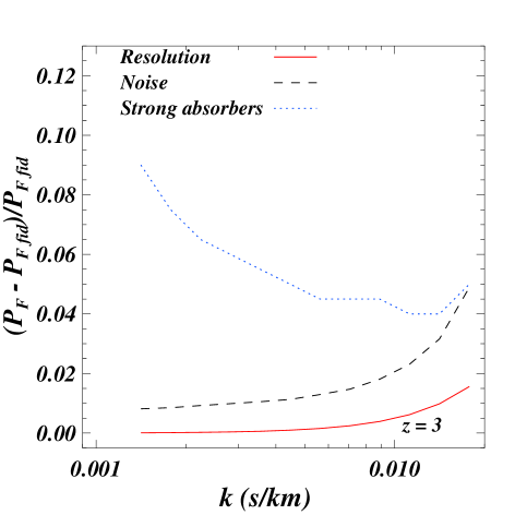
M04b have applied a number of corrections for noise, resolution and the correlated SiIII feature identified by M04a. We have adopted the same corrections which are summarized below. For more details we refer to M04a and M04b. We allow for an error in the dependent noise correction at each redshift by subtracting from and treat the as free parameter in the fit. M04b recommend to assume that the distribution of is Gaussian with mean zero and width 0.05 which corresponds to a typical error in the noise correction of . M04a further recommend to allow for an overall error on the resolution correction, by multiplying with , where is treated as a free parameter with Gaussian distribution with mean zero and width . To account for contamination by the correlated SiIII feature we modify our model flux power spectra as suggested as follows, with , and km/s. The noise and resolution corrections and their errors depend strongly on the wavenumber as shown in Figure 1. Note that M04a also subtracted a contribution of uncorrelated associated metal absorption which they estimated redward of the Lyman- emission line. The effect of continuum fitting errors on the flux power spectrum is a further uncertainty which is discussed in K04, M04a and Tytler et al. (2004). Continuum fitting errors are difficult to quantify and we again follow M04b in not attempting to model them.
4.2.2 Uncertainty of the effective optical depth
As discussed in VHS and Seljak et al. (2003) the poorly known effective optical depth results in major uncertainties in any analysis of the Lyman- forest flux power spectrum. The effective optical depth is to a large extent degenerate with the amplitude of the matter power spectrum. As shown in M04b the dependence of changes in the flux power spectrum due to varying effective optical depth and amplitude of the matter power spectrum are, however, somewhat different. This allows – at least in principle – to break this degeneracy. We will come back to this point later. When modelling the effective optical depth we will investigate two cases. We will either let the effective optical depth vary independently in the different redshift bins or we will parameterize the evolution of the effective optical depth as a power law in redshift.
4.2.3 Uncertainties due to the thermal state of the IGM
In order to explore in more detail the uncertainties due to thermal effects on the flux power spectrum we have run simulations with a wide range of thermal histories (Table 1). Note that this is different from VHS where we have only performed a-posteriori rescalings of the temperature-density relation to investigate thermal effects. We have calculated the value as the median temperature of gas with logarithmic overdensity values between -0.1 and 0.1. The value of we determined from the slope of the temperature-density relation for gas at mean density and 1.1 times the mean density.
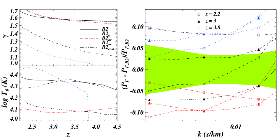
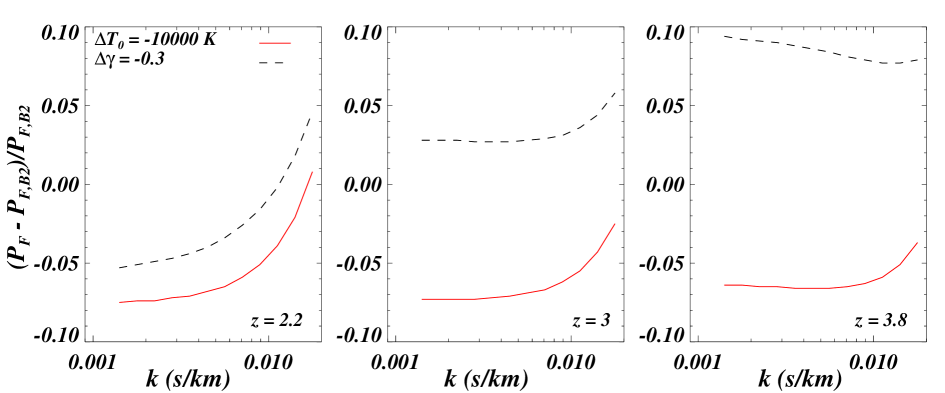
In the left panel of Figure 2 we plot the different thermal histories (temperature at mean density in the bottom panel and in the top panel). The linestyles denote the different models as follows. The continuous curve is our standard B2 model with the equilibrium solver. The dashed curves shows the same model with the non-equilibrium solver () which results in a significantly smaller . The dotted and dot-dashed and curve shows the same model with the non-equilibrium solver for late reionization at () and early reionization at (). Finally, the dashed-triple-dot curves shows a model with reionization at but smaller heating rate and thus a lower temperature, similar to that of .
In the right panel we show the differences of the flux power spectrum relative to our fiducial model at three different redshifts. The differences are typically %. Comparing and , which have a similar redshift evolution we find for example that a decrease of by 50% ( K) results in a decrease in the flux power larger than . The effect of changing can be judged by comparing and at which have approximately the same temperature. Decreasing by produces an increase in the flux power by 7.5 % (2.5 %), but we note that for s/km the differences increase strongly.
We will later model the evolution of the thermal state of the IGM with redshift as broken power laws for temperature and slope of the temperature-density relation.
4.2.4 Uncertainties due to the modelling of the flux power spectrum
Modelling the flux power spectrum accurately is numerically challenging and checks for convergence are important. We have chosen to use here full hydro-simulations performed with GADGET-2 described in section 3. In VHS we found that simulations with a box size 60 Mpc and with particles (60,400) are the best compromise for the analysis of the LUQAS sample. The lower resolution SDSS power spectrum is not affected on large scale in the same way by continuum fitting errors as the high-resolution spectra which we used in VHS and for which continuum fitting errors appear to increase the flux power significantly at and above the scale corresponding to one Echelle order (Kim et al. 2004). The usable range of wavenumbers is thus shifted to larger scales compared to flux power spectra obtained from high-resolution Echelle data. Ideally one would thus like a somewhat larger box size than that used in VHS. Unfortunately this is currently not feasible with simulations that at least marginally resolve the Jeans length. We have thus decided to use simulations with the same box size and resolution as in VHS.
Box size : For the final analysis we use simulations of 60 Mpc and with particles (60,400). Since the error bars for the observed 1D flux power spectrum are significantly smaller than those of the 3D flux power used by VHS we checked whether or not the flux power spectrum is affected by box size and/or limited resolution at the percent level. We have first checked how well the largest scales probed by SDSS are sampled by our fiducial (60,400) simulations. In VHS this was not an issue since the first data point used in the analysis was at s/km, which was well sampled by the (60,400) simulations. Our analysis here extends however to s/km and could be affected by cosmic variance. To test this, we have compared the flux power spectrum of our fiducial (60,400) simulation B2 with that of a (120,400) simulation of the same model (B2120,400). The power of the latter at s/km is typically larger by % at , respectively. We correct for this by multiplying the flux power spectrum of the (60,400) simulation by corresponding factors. We will later use simulations with a factor two smaller box size but the same resolution as our fiducial simulation to explore the effects of the thermal history. We have thus also compared the flux power spectrum of our fiducial (60-400) simulation B2 with a (30-200) simulation of the same model (B230,200) and find that the latter underestimates the power by in the range (s/km) at . Our findings regarding the dependence of the flux power spectrum on the thermal history of the IGM should thus be little affected by the fact that they were obtained from simulations of smaller box size.
Resolution : To quantify the effect of resolution, we compare the simulation B230,200 with B230,400 a simulation which has the same box sixe but eight times better mass resolution. The differences between B230,400 and B230,200 are less than 5 % for (s/km), at any redshift, (3% in the range (s/km) ). At s/km, the flux power spectrum of B230,400 is larger by , at and , respectively. This is in agreement with the findings of M04b. We will correct for the limited resolution by multiplying the flux power spectrum of our fiducial (60,400) simulation by corresponding factors. Both the resolution and box size errors are comparable or smaller than the statistical errors of the flux power spectrum. We explicitly checked that these corrections do not significantly affect the parameters of our best-fitting model. They do, however, affect the value of the best-fitting model. Note that both the resolution and box size corrections could be model dependent.
High Column density systems/Damped Lyman- systems: We have recently pointed out that the absorption profiles of high column density systems/damped Lyman- systems have a significant effect on the flux power spectrum over a wide range of scales (Viel et al. 2004b). These absorption systems are caused by high-redshift galaxies and the gas in their immediate vicinity. Numerical simulations still struggle to reproduce these systems correctly and they are thus a major factor of uncertainty in modelling the flux power spectrum. M04b have modelled the expected effect on the SDSS flux power spectrum and we have included this correction using the k-dependence of Fig. 11 in M04b. M04b recommend to assume that the distribution of the correction made is Gaussian with mean 1 and width 0.3. The correction is shown in Figure 1 as the dotted curve. It is of order of % at the largest scales and drops to 3% at the smallest scales. Note that unlike M04b we have assumed that this correction does not vary with redshift.
4.2.5 Uncertainties due to UV fluctuations, galactic winds, reionization history, temperature fluctuations
There are a range of physical processes some of which are difficult to model, that are described below. Note that we have chosen not to try to include these effects in our analysis.
Spatial fluctuations of the ionization rate: The flux power spectrum is obviously sensitive to the neutral fraction of hydrogen which depends on the ionization rate. At low redshift the mean free path of ionizing photons is sufficiently large that spatial fluctuations of the rate should be too small to affect the flux power spectrum relevant for our investigation here (Meiksin & White 2004; Croft 2004; McDonald et al. 2005). At higher redshift this is less obvious. Quantitative modelling of the fluctuations requires however a detailed knowledge of the source distribution of ionizing photons which is currently not available. As we will discuss below there may be some tentative evidence that UV fluctuations do become important at the highest redshifts of the SDSS flux power spectrum sample.
Galactic Winds: There is undeniable observational evidence that the Lyman- forest has been affected by galactic winds. Associated metal absorption is found to rather low optical depth (Cowie et al. 1995, Schaye et al. 2003). Searches for the effect of galactic winds on QSO absorption spectra from Lyman break galaxies close to the line-of-sight have also been successful. The volume filling factor of galactic winds and the material enriched with metals is, however, very uncertain (e.g. Pieri & Haehnelt 2004; Adelberger et al. 2005; Rauch et al. 2005). Numerical simulations have generally shown the effect of galactic winds to be small (Theuns et al. 2002a; Kollmeier et al. 2003; Desjacques et al. 2004; McDonald et al. 2005; Kollmeier et al. 2005).
Temperature fluctuations:
It is rather difficult to measure mean values of the temperature and little is known observationally about spatial fluctuations of the temperature (Theuns et al. 2002b). In the redshift range of interest the heating rate of the IGM should be dominated by photo-heating of helium before helium is fully reionized. Helium reionization should thus lead to spatial temperature fluctuations (Miralda-Escudé et al. 2000), which will affect the neutral fraction of hydrogen through the temperature dependence of the recombination coefficient. Temperature fluctuation may thus affect the flux power spectrum. Quantitative modelling of their effect on the flux power spectrum requires numerical simulation of helium reionization including full radiative transfer and good knowledge of the spatial distribution of the source of ionizing photons. Such modelling will also be uncertain.
Reionization history: The flux power spectrum is not only sensitive to the current thermal state of the IGM but also to its past thermal history. This is because the spatial distribution of the gas is affected by pressure effects (Hui & Gnedin 1997; Theuns, Schaye & Haehnelt 2000; Zaldarriaga, Scoccimarro, Hui 2001). Quantitative modelling of this effect is, however, again very uncertain as the heating rate at high redshift is expected to be dominated by photo-heating of helium. In order to get a feeling for the effect of a simple change of the redshift when reionization occurs we can compare and at . Both simulations have approximately the same values for and at while reionization occurs at and , respectively. The differences are of the order of 3%, in agreement with the findings of M04a.
4.3 Finding a “best guess” model
In order to settle on a best guess model we have started with the coarse grid of hydro-simulations presented in VHS. We have complemented this with simulations of a wider range of and a wider range of thermal histories. We have fitted the flux power spectrum of all (60,400) simulations listed in Table 1 to the SDSS flux power spectrum allowing for errors in the correction to the data as described in section 4.2.1. We thereby leave the effective optical depth as a free parameter at all redshifts.
The last column in Table 1 gives the resulting values obtained using the full covariance matrix as given by M04a 111http://feynman.princeton.edu/pmcdonal/LyaF/sdss.html. When performing the fits we noticed that the highest redshift bin at is generally fitted very poorly. Omitting these 12 data points usually reduced the by about 26 for 11 degrees of freedom (d.o.f.). This may either indicate some problem with the data or some insufficiency of the model. The latter would require, however, a very rapid change of the model with redshift as dropping any of the other redshift bins reduced the by the expected amount. UV fluctuations are probably the most plausible candidate for a rapid change toward the highest redshift bin. We have decided to drop the highest redshift bin for our analysis. This leaves 96 data points and 8 free (unconstrained) parameters corresponding to 88 degrees of freedom.
The best fitting simulation appears to be B2.5 which has , when minimizing over the noise array , the resolution and the effective optical depth. The simulation B2 has a close to that of B2.5, while the other models have typically . We regard these two models, with their thermal history, as reasonable good fits to the data set ( values higher than the quoted values have a probability of 16% and 11% to occur).
We decided to choose B2 as our best guess model despite the fact B2 has a somewhat larger value than B2.5 for two reasons. First, the model is surprisingly close to the best fit model quoted by M04a (which has , , and ). Secondly, we had already run more simulations exploring different thermal histories for B2 than for the other models. We have, however, checked as discussed in more detail in section 5 that an expansion around the B2.5 model gives essentially the same results in terms of the inferred astrophysical and cosmological parameters.
4.4 Derivatives of the flux power spectrum of the “best guess” model
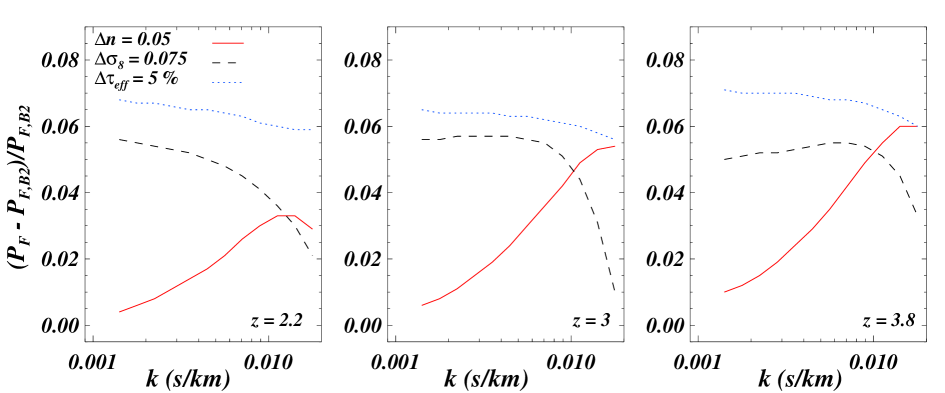
The key ingredient for our estimates of a fine grid of flux power spectra are the derivatives of the flux power spectrum (see equation 1) close to the best guess model B2. Figure 3 shows the dependence of the most relevant of these derivatives at three redshifts ( from left to right) in the form of the change of the flux power spectrum for a finite change of the parameters. We compute these derivatives at the wavenumbers of the SDSS flux power spectrum, although we cannot directly cover the two smallest wavenumbers because we are using (30,200) simulations to estimate these derivatives. For these two points we have used an extrapolation with a 2nd order polynomial. This should be a reasonable approximation given the rather weak and smooth dependence at these scales.
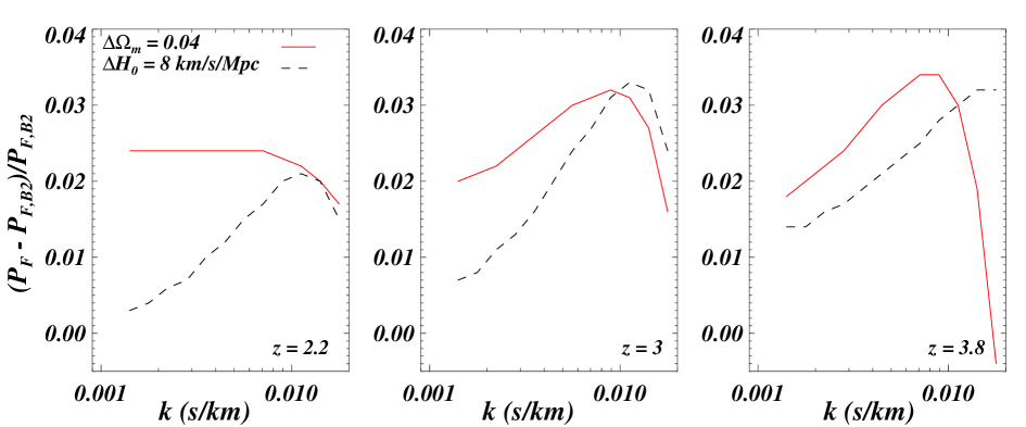
In the top panel we show how the flux power spectrum depends on , , . A increase in the effective optical depth, translates into a 7% increase in the flux power spectrum with no dependence on redshift and with very little () dependence on wavenumber. A change of the spectral index by leads to an increase of the flux power which rises steeply with wavenumber from to , while increasing by 9% increases the flux power by for (s/km) dropping to at the smallest scales considered here. The changes introduced by different values of and are shown in the middle panel. An increase of the Hubble parameter by 8 km/s/Mpc leads to an increase of order 3%, while the change due to an increase of shows a peaks at s/km of 3% at and depends less strongly on wavenumber at lower redshifts. The derivatives of the flux power spectrum with respect to changes in temperature and power-law index of the temperature density relations are shown in the bottom panel. The trends are the same as those shown in Figure 2. We note that the overall effect depends only weakly on wavenumber for s/km and steepens at smaller scales. Note that the dependence of the derivatives on and is distinctively different for the different parameters. This is the reason why we will be able to obtain reasonably tight constraints for most of them.
Our results agree quite well with the results of VHS and M04b. We note, however, that a direct quantitative comparison with M04b is not obvious. Our best guess model has still somewhat different parameters from their fiducial model and M04b have used HPM simulations with a range of corrections while we have used full hydro-simulations. One may ask how much these derivatives depend on our choice of the best-guess model. We have checked this for a few cases. The derivatives obtained by rescaling the effective optical depth around other models (B1,B3,C3) are different by less then 0.5 % compared to those shown in Figure 3. The derivatives with respect to and differ by less than 2.5% and 1.5 %, respectively, compared to expanding around B2. We have also directly compared the approximate flux power obtained with the Taylor expansion with that extracted from hydrodynamical simulations for a few simulation with parameters that are about away from our best-guess model. For the and (60,400) the error of the aproximation is less than 3.5% which should be compared to the difference to the best-guess model which is %. We have also run a few further (30,200) simulations with , and a hotter simulations with =41000 K and . The approximations for the models with different and the spectral index are accurate to 1%. The error for the model with the different parameter is %. By comparing with Figure 3 we find that for displacements in the parameters ,, and the error of the Taylor series approximation is generally less than 30% of the difference between the models. This is not perfect but should be acceptable considering the expense of full-hydrodynamical simulations and the size of the parameter space.
5 Constraining Astrophysical and Cosmological Parameters
5.1 Summary of the free parameters of the minimization
We have modified the code COSMOMC (Lewis & Bridle 2002) to run Monte Carlo Markov Chains for our set of parameters. After settling on a best guess model we have explored the parameter space close to the best guess model. For most of the analysis we have used 22 parameters for the minimization, some of them free some of them independently constrained. We briefly summarize the parameters here.
We assume a flat cosmological model with a cosmological constant and neglect the possibility of a non-zero neutrino mass. There are thus four cosmological parameters that describe the matter distribution: the spectral index , the dark matter power spectrum amplitude , and . We use nine “astrophysical” parameters. Two describe the effective evolution of the optical depth evolution, six describe the evolution of and and one describes the contribution of strong absorption systems. For the evolution of the optical depth we assume a power-law . Note that this is different from what we did when we fitted the suite of hydro-simulations where we let the effective optical depth vary independently at all redshift bins. We will come back to this in section 5.4.
For the evolution of and we assume broken power-laws with a break at . The three parameters for the temperature are the amplitude at , and the two slopes and . is described in the same way by , and . The correction for the damped/high column density systems is modelled with the dependence of Figure 11 of M04b and an overall amplitude and no redshift evolution, as described in section 4.2.4.
Finally, we have a total of 9 parameters which model uncertainties in the correction to the data. Eight parameters for the noise correction as described in section 4.2.1 and one parameter describing the error of the resolution correction. Note that all the parameters describing the errors of the corrections to the data and the correction for damped/high column density systems are constrained as suggested in M04b and described in section 4.2.
We will present here two sets of results. At first we will discuss the 1D and 2D likelihoods for the most significant parameters by assuming no priors on the cosmological and astrophysical parameters (with the exception of the correction for damped systems). Then we will show some results assuming priors on the Hubble parameter and on the thermal history.
5.2 Results without priors
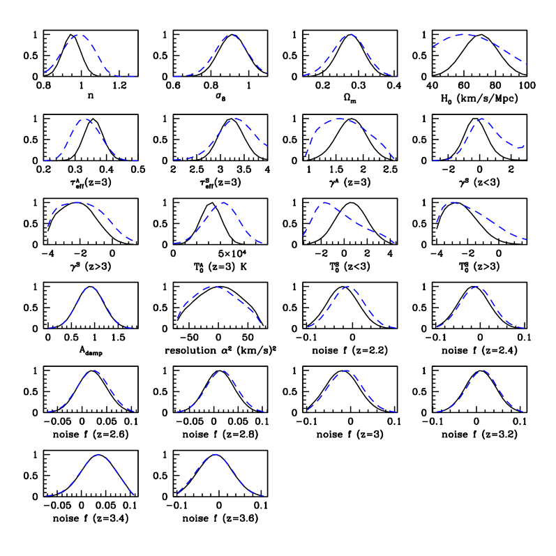
The dashed curves in Fig. 4 show the 1D (marginalized) likelihoods for our full set of parameters without imposing any priors on the cosmological and astrophysical parameters. The best fit model has now for 84 d.o.f.. A equal or larger than this should have a probability of 64%. Our best-fitting model is thus an excellent fit, maybe with a hint that we are already marginally over-fitting the data. Most parameters including , and are tightly constrained. The constraints on the thermal history are considerable weaker. This is not surprising as the rather low resolution of the SDSS spectra means that the thermal cut-off at small scales is not actually resolved. The best fit value for is rather high, K, and may be in disagreement with the best fit values of M04b who find K without giving any error estimate.
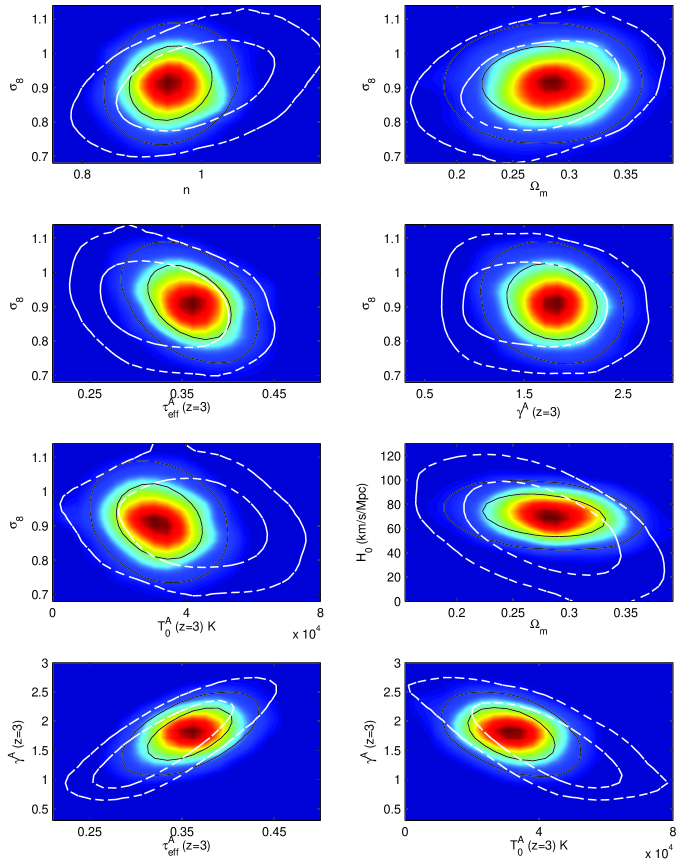
The dashed curves in Figure 5 show 2D likelihood contours for various parameter combinations. The contours have been obtained by marginalizing over the rest of the parameters. We note that the best fit models prefer somewhat larger values of the spectral index and higher temperatures than those of our best guess model. The 2D contour plot of vs , suggests that in order to reconcile this measurement with a colder IGM one would need an unplausibly steep temperature density relation with .
The preferred values for the thermal state of the IGM are actually outside the range suggested by a detailed analysis of the line width of the absorption feature using high-resolution spectra. This is shown in Figure 6 where we compare the best-fitting evolution of the temperature (hashed region) to the measurements of the temperature by Schaye et al. (2000). Note again that the lower range of values corresponds to outside of the range of plausible values for a photoionized IGM. The Hubble constant is also only poorly constrained. This is again not surprising as the spectra are sensitive to the matter power spectrum in velocity space. The only dependence comes thus through the shape parameter , which is weak (3).
The best fitting values for our modelling without priors with errors obtained by marginalizing over all other parameters are listed in Table 2.
As a further consistency check and to test how well the observed redshift evolution of the flux power spectrum probes the expected gravitational growth of structure we have also obtained constraints on and independently for each redshift bin. We get the following constraints for : , , , , , , , , , for , respectively. For we get: , , , , , , , , for , respectively. The total is . for 74 d.o.f. in this case. The constraints are weaker but perfectly consistent with our estimates from all redshift bins combined. The errors are significantly smaller than the expected growth of the amplitude between the lower and upper redshift end of the sample demonstrating that the flux power spectrum evolves as expected for gravitational growth.
| parameter | without priors | with priors on thermal |
|---|---|---|
| history and | ||
| n | ||
| (km/s/Mpc) | ||
| K | ||
5.3 Results with priors
As discussed in the last section the SDSS flux power spectrum of SDSS published by M04a prefers unplausibly large temperatures for reasonable values of . We have thus repeated the analysis with (Gaussian) priors on the thermal state of the IGM, as follows, , and (Schaye et al. 2000). We have also added a prior on the Hubble constant, km/s/Mpc (Freedman et al. 2001).
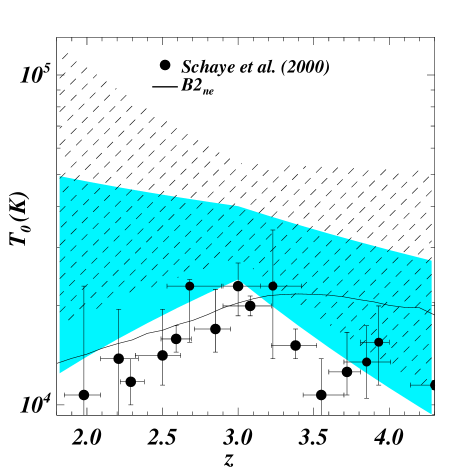
The solid curves in Figure 4 and Figure 5 show the marginalized likelihoods for our analysis with priors. The filled (coloured) contours in Figure 5 show the mean 2D likelihood. As expected the thermal parameters and the Hubble constant are now more tightly constrained. The temperature evolution of the best-fitting model with prior is shown as the shaded region in Figure 6. It lies about 1 above the imposed constraint suggesting that the observed flux power spectrum definitely prefers models with higher temperatures than those observed. Rather than being an actual indication of higher temperature this is more likely indicative of a not understood systematic uncertainty in our modelling which makes the flux power spectrum mimic high temperatures. As discussed in section 4.2.5 there are plenty of candidates for this.
The best fit model with priors has For 88 degrees of freedom. A equal or larger than this should have a probability of 60% very similar to the case without priors. The best fitting values for our modelling without priors are also listed in Table 2 (right column).
The most significant change caused by the introduction of the priors is a decrease of the spectral index by (consistent with the errors). In Figure 5 the strongest correlations are those in the , and planes. As expected a higher value of the requires a smaller quantitatively comparable to previous findings (Viel, Weller & Haehnelt 2004; VHS; Seljak et al. 2003). The best-fitting temperature and slope of temperature density relation are again anti-correlated. A lower temperature corresponds to a steeper temperature density relation. We further note that and appear not to be correlated, in contrast to the corresponding parameters in M04b. If we take out the box size and resolution corrections we do not get significant changes in the final parameters but the increases by 1.3, showing that the data prefer these corrections. The best fitting values for our modelling with priors with errors obtained by marginalizing over all other parameters are also listed in Table 2.
5.4 The inferred evolution of the effective optical depth
As discussed before the effective optical depth is the largest uncertainty and it is very degenerate with the fluctuation amplitude. Larger effective optical depths correspond to smaller values (Figure 5). The shape of the derivative of the flux power spectrum with respect to and (Figure 3) is, however, sufficiently different to get still interesting constraints on .
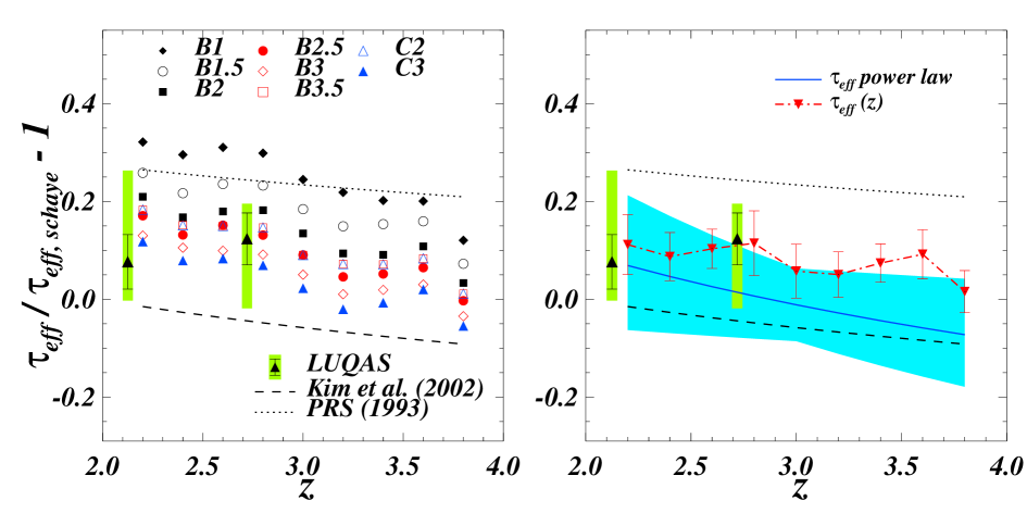
In the left panel of Figure 7 we compare the best fitting for our set of (60,400) hydrodynamical simulations to measurements made from high and low resolution spectra. All values are shown relative to the fit to the observed evolution of the optical depth corrected for the contribution by associated metal absorption based on a set of high-resolution spectra by Schaye et al. 2003 (their Figure 1). The fit is given by . The evolution obtained by Kim et al. (2002) based on a different set of high-resolution spectra is shown as the dashed curve. The measurements at and made by VHS from the LUQAS sample (Kim et al. 2004) are shown as filled triangles. Note that there is some overlap between the Schaye et al. (2003) data set and the LUQAS sample of K04. The dotted line shows the result of Press, Rybicki & Schneider (PRS, 1993) from low-resolution spectra of rather poor quality. The shaded area shows the range adopted by VHS and Viel, Weller & Haehnelt (2004) for their analysis. The different symbols show the results from our fits of the flux power spectrum of the hydro-simulations to the SDSS flux power spectrum as described in section 4.3. The degeneracy between and is clearly visible and can be roughly described by similar to that found in VHS.
In the right panel, the solid curve shows the evolution of for our best fitting model compared to the same observational estimates. As discussed we have modelled the evolution of as a power-law. We find in agreement with Schaye et al. (2003) and the values used by VHS. It also agrees well with the values inferred by Lidz et al. (2005) from the flux probability distribution. The shaded area in the right panel shows the uncertainty of the best fitting model. We thus confirm the findings of M04b that the differences in the dependence of the respective changes can break the degeneracy between and . The dot-dashed line and the triangles show the evolution of the optical depth if we let vary separately at all nine redshifts (this increases the number of free parameters from 22 to 28). Letting the effective optical depth vary freely at high redshift increases the average inferred effective optical depth by about 5% and reduces the inferred errors.
| Spergel et al. (2003)(a) | ||
|---|---|---|
| Spergel et al. (2003)(b) | – | |
| Viel, Haehnelt & Springel (2004)(c) | ||
| Viel, Weller & Haehnelt (2004)(d) | ||
| Desjacques & Nusser (2004) | – | |
| Tytler et al. (2004) | 0.90 | – |
| McDonald et al. (2004b)(e) | ||
| Seljak et al. (2004)(f) | ||
| This work (priors case) |
-
(a) WMAP only, (b) WMAPext +2dF +
Lyman- (no running of the spectral index),(c)
LUQAS+Croft et al. (2002) only; (d) LUQAS+Croft et al. (2002) + WMAP 1st year; (e) error bars extrapolated by the authors from the abstract of M04b; (f) SDSS Lyman- flux power spectrum + WMAP.
6 Discussion and Conclusion
6.1 Comparison with previous results for and
In Table 3 we list results for the most important parameters describing the matter distribution ( and ) obtained by recent studies using the Lyman- forest by a variety of authors. The most direct comparison is again with M04b. At our results correspond to an fluctuation amplitude and effective slope at the pivot wavenumber s/km as defined by M04b of and . The values are consistent within with those of M04b. The agreement with otherauthors including our own work is at the same level. For comparison we also show the value for WMAP alone. A consistent picture emerges for the Lyman- forest data with a rather high fluctuation amplitude and no evidence for a significant deviation from or a running of the spectral index. This results holds for the Lyman- forest data alone but is considerably strengthened if the Lyman- forest data is combined with the CMB and other data.
6.2 Remaining Uncertainties and Future Progress
As discussed in section 4.2 there are many systematic uncertainties that affect the measurement of cosmological parameters with the Lyman- flux power spectrum.
In order to test the stability of the results we have removed the correction for high column density systems and the errors for the noise and resolution corrections in the case with priors. If we take out the correction due to strong absorption systems , decreases to , and the best fit value for becomes 0.381, all the other parameters remain practically unchanged. The measured values do therefore practically not change but the value of increases by 0.5. If we do not allow for the error to the noise and resolution corrections the inferred values do again not change but the value of increases by 1.8. Note that M04a have also subtracted an estimate of the contribution of associated metal absorption from the flux power spectrum and have applied a suite of other (smaller) corrections to the data (see M04a for more details). Many of these corrections would either not be necessary or substantially easier for spectra with somewhat better resolution () and higher S/N. Obtaining large samples of such spectra is observationally feasible and there is certainly room for improvement. Note further that the SDSS team will soon release a further measurement of the flux power spectrum performed by an independent group within the collaboration.
We also note again that calculating the flux power spectrum by using a Taylor expansion to first order around the best guess model is just an approximation. This was an important part of our analysis as it reduced the amount of CPU time necessary dramatically, but could be further improved by getting more accurate fits around the “best guess” model. We have also not attempted to correct for the possible effects of spatial fluctuations of the ionization rate, galactic winds, temperature fluctuation or the reionization history. This is because we are not convinced that it is already possible to model these effects with sufficient accuracy. This should hopefully change in future with improved observational constraints and numerical capabilities. One should further keep in mind that so far very little cross checking of hydrodynamical simulation run with different codes has been performed.
In our study the rather poorly known thermal state of the IGM is one of the major remaining uncertainties. Further high-resolution spectroscopy and improved modelling will hopefully soon improve this. Accurate modelling of the effect of high column density systems/ damped Lyman- systems and improvement in the determination of the column density distribution of observed absorption systems in the poorly determined range around should also be a priority in further studies (see the discussion in McDonald et al. 2005).
It is certainly encouraging that the differences between our analysis and that of M04b are moderate despite considerable differences between their approximate HPM simulations calibrated with hydrodynamical simulations of rather small box size and our analysis with full hydrodynamical simulations of much larger box size here and in VHS.
For the time being we would advice the conservative reader to double the formal errors quoted here. This will bring the error estimates to about the same size as the also conservative estimates for the errors of the fluctuation amplitude from the Lyman- forest data alone in the analysis of VHS. The actual errors lie probably somewhere in between.
6.3 Conclusions
We have compared the flux power spectra calculated from a suite of full large box-size high resolution ( Mpc, particles) hydrodynamical simulations with the SDSS flux power spectrum as published by McDonald et al. (2005). We have identified a best-guess model which provides a good fit to the data. We have used a Taylor expansion to first order to calculate flux power spectra in a multi-dimensional space of parameters describing the matter power spectrum and the thermal history of the IGM with values close to those of our best-guess model. We have investigated the combined effect of cosmological and astrophysical parameters on the flux power spectrum with an adapted version of the Markov-Chain code COSMOMC. Our main results can be summarized as follows.
-
•
The flux power spectrum calculated directly from the simulation of a CDM model (, , and , ) with a temperature density relation described by and gives an acceptable fit to the SDSS flux power spectrum in the redshift range ( for 88 degrees of freedom). The fit can easily be further improved by small changes in the cosmological and astrophysical parameters.
-
•
At higher redshift the deviations from the observed flux power spectrum become significantly larger ( for 12 additional data points at ) suggesting either some problem with the data or a physical effect that changes rapidly with redshift.
-
•
We confirm the claim by McDonald et al. (2004) that the degeneracy of the dependence of the flux power spectrum on the amplitude of the matter power spectrum and the effective optical depth can be broken for the published SDSS flux power spectrum. It will be interesting to see if the same is true for the independent analysis of the SDSS data to be released soon.
-
•
The SDSS power spectrum alone can constrain the amplitude of the matter power spectrum, the matter density and the power-law index of primordial density fluctuation to within . The thermal state of the IGM is however, poorly constrained and the SDSS power spectrum formally prefers models with unplausible values of the parameters describing the thermal state. The dependence of the flux power spectrum on the assumed Hubble constant is also very weak and the Hubble constant is not well constrained. The exact values for the other cosmological parameters depend somewhat on the assumed prior for the thermal state and the details of the correction which have been applied to the data.
-
•
With a prior on the thermal history and the Hubble constant motivated by the observations by Schaye et al. (2000) and Freedman et al. (2001) we obtain the following best-fitting values for the cosmological parameters , , ( error bars), and the effective optical depth is well described by the following power-law relation: . The errors were obtained by marginalizing over a set of 22 parameters describing the matter distribution, thermal history of the Universe, the effective optical depth and errors to various corrections to the data. The values for and are consistent with those found by M04a for the same data set with different simulations. They are also consistent with the results of other recent studies of Lyman- forest data. The inferred optical depth is in good agreement with that measured directly from continuum-fitted high-quality absorption spectra.
Acknowledgments.
The simulations were run on the COSMOS (SGI Altix 3700) supercomputer at the Department of Applied Mathematics and Theoretical Physics in Cambridge. COSMOS is a UK-CCC facility which is supported by HEFCE and PPARC. MV thanks PPARC for financial support. We thank James Bolton for providing us with the non-equilibrium solver for GADGET-2 , Antony Lewis for useful suggestions and technical help and the anonymous referee for useful suggestions.
References
- [] Abel T., Haehnelt M.G., 1999, ApJ, 520, 13
- [] Adelberger et al., 2005, astro-ph/0505122
- [] Bolton J.S., Haehnelt M.G., Viel M., Springel V., 2005a, MNRAS, 357, 1178
- [] Bolton J.S., Haehnelt M.G., Viel M., Carswell R.F., 2005b, arXiv: astro-ph/0508201
- [] Cowie L., Songaila A., Kim T.-S., Hu E.M., 1995, AJ, 109, 1522
- [] Croft R. A. C., 2004, ApJ, 610, 642
- [] Croft R. A. C., Weinberg D. H., Katz N., Hernquist L., 1998, ApJ, 495, 44
- [] Croft R. A. C., Weinberg D. H., Bolte M., Burles S.,Hernquist L., Katz N.,Kirkman D., Tytler D., 2002, ApJ, 581, 20 [C02]
- [] Desjacques V., Nusser A., 2005, arXiv:astro-ph/0410618
- [] Desjacques V., Nusser A., Haehnelt M. G., Stoehr F., 2004, MNRAS, 350, 879
- [] Eisenstein D. J., Hu W., 1999, ApJ, 511, 5
- [] Freedman W.L. et al., 2001, ApJ, 553, 47
- [] Gnedin N. Y., Hui L., 1998, MNRAS, 296, 44
- [] Gnedin N. Y., Hamilton A. J. S., 2002, MNRAS, 334, 107
- [] Haardt F., Madau P., 1996, ApJ, 461, 20
- [] Hui L., Gnedin N., 1997, MNRAS, 292, 27
- [] Hui L., Burles S., Seljak U., Rutledge R. E., Magnier E., Tytler D., 2001, ApJ, 552, 15
- [1] Lewis A., Bridle S., 2002, Phys. Rev., D66, 103511; http://www.cosmologist.info
- [] Lidz A., Heitmann K., Hui L., Habib S., Rauch M., Sargent W.L.W., 2005, astro-ph/0505138
- [] Kim, T.-S., Carswell, R. F., Cristiani, S., D’Odorico, S., Giallongo, E. 2002, MNRAS, 335, 555
- [] Kim, T.-S., Viel M., Haehnelt M.G., Carswell R.F., Cristiani S., 2004, MNRAS, 347, 355 [K04]
- [] Kollmeier J.A., Weinberg D.H., Davé R., Katz N., ApJ, 594, 75
- [] Kollmeier J., Miralda-Escude J., Cen R., Ostriker J.P., 2005, ArXiv: astro-ph/0503674
- [] McDonald P., 2003, ApJ, 585, 34
- [] McDonald P., Seljak U., Cen R., Bode P., Ostriker J.P., 2005, MNRAS, in press
- [] McDonald P., Miralda-Escudé J., Rauch M., Sargent W.L., Barlow T.A., Cen R., Ostriker J.P., 2000, ApJ, 543, 1
- [] McDonald P. et al., 2004a, astro-ph/0407377 [M04a]
- [] McDonald P. et al., 2004b, astro-ph/0407378 [M04b]
- [] Meiksin A., White M., 2004, MNRAS, 350, 1107
- [] Pieri M., Haehnelt M.G., 2004, 347, 985
- [] Press W. H., Rybicki G. B., Schneider D. P., 1993, ApJ, 414, 64
- [] Rauch M. et al., 2005, ApJ, in press
- [] Ricotti M., Gnedin N., Shull M., 2000, ApJ, 534, 41
- [] Schaye J., Theuns T., Rauch M., Efstathiou G., Sargent W. L. W., 2000, MNRAS, 318, 817
- [] Schaye J., Aguirre A., Kim T.-S., Theuns T., Rauch M., Sargent W. L. W., 2003, ApJ, 596, 768
- [] Seljak U., McDonald P., Makarov A., 2003, MNRAS, 342, 79L
- [] Seljak et al., 2004, astro-ph/0407372
- [] Spergel D. N. et al. 2003, ApJS, 148, 175
- [] Springel V., 2005, astro-ph/0505010
- [] Springel V., Hernquist L., 2002, MNRAS, 333, 649
- [] Springel V., Yoshida N., White S.D.M., 2001, NewA, 6, 79
- [] Theuns T., Schaye J., Haehnelt M.G., 2000, 315, 600
- [] Theuns T., Leonard A., Efstathiou G., Pearce F.R., Thomas P.A., 1998, MNRAS, 301, 478
- [] Theuns T., Zaroubi S., Kim T.-S., Tzanavaris P., Carswell R.F., 2002b, MNRAS, 332, 367
- [] Theuns T., Viel M., Kay S., Schaye J., Carswell B., Tzanavaris P., 2002a, ApJ, 578, L5
- [] Tytler et al., 2004, ApJ, 617, 1
- [] Verde L., et al. 2003, ApJS, 148, 195
- [] Viel M., Haehnelt M.G., Springel, 2004, MNRAS, 354, 684 [VHS]
- [] Viel M., Weller J., Haehnelt M.G., 2004, MNRAS, 355, 23L
- [] Viel M., Haehnelt M.G., Springel, 2005, astro-ph/0504641
- [] Viel M., Haehnelt M. G., Carswell R. F., Kim T.-S., 2004b, MNRAS, 349, L33
- [] Viel M., Matarrese S., Theuns T., Munshi D., Wang Y., 2003, MNRAS, 340, L47
- [] Viel M., Lesgourgues J., Haehnelt M.G., Matarrese S., Riotto A., 2005, Phys.Rev.D71, 063534
- [] Zaldarriaga M., Hui L., Tegmark M., 2001, ApJ, 557, 519
- [] Zaldarriaga M., Scoccimarro R., Hui L., 2003, ApJ, 590, 1