A Potential Supernova Remnant/X-ray Binary Association in M31

Abstract

The well-studied X-ray/Optical/Radio supernova remnant DDB 1-15 (CXOM31 J004327.8+411829; r3-63) in M31 has been investigated with archival XMM-Newton and Chandra observations. The timing data from XMM-Newton reveals a power density spectrum (PDS) characteristic of accreting compact objects in X-ray binaries (XRBs). The PDS shows features typical of Roche lobe overflow accretion, hinting that the XRB is low-mass. The Chandra observations resolve the SNR into a shell and show a variable count rate at the 94% confidence level in the northwest quadrant. Together, these XMM-Newton and Chandra data suggest that there is an XRB in the SNR r3-63 and that the XRB is located in the northwestern portion of the SNR. The currently-available X-ray and optical data show no evidence that the XRB is high-mass. If the XRB is low-mass, r3-63 would be the first SNR found to contain a low-mass X-ray binary.

1 Introduction

Neutron stars and black holes are thought to form in core-collapse supernova (SN) explosions. In recent years, several neutron stars have been found as X-ray point sources within supernova remnants (SNR) by Chandra (e.g., G292.0+1.8 Hughes et al., 2001; G0.9+0.1 Gaensler et al., 2001; CTA 1 Halpern et al., 2004), but none of these compact objects has been in a binary system. Only a single supernova remnant/X-ray binary (SNR/XRB) association is known in the Galaxy, and that is the association between the high-mass X-ray binary (HMXB) SS 433 and the SNR W50 (Geldzahler et al., 1980).

Some possible extragalactic SNR/XRB associations have been discovered in recent years. Roberts & Colbert (2003) inferred a black hole XRB in the ultra-luminous SNR MF16 in the galaxy NGC 6946, and Chu et al. (2000) identified a possible SNR/XRB pair in the LMC (RX J050736-6847.8). Additionally, Coe et al. (2000) suggested XTE J0111.2-7317 in the SMC as a possible Be XRB in a SNR. None of these systems contain a low-mass X-ray binary (LMXB). The reason that there are so few known SNR/XRB associations and no known SNR association with a LMXB is unclear.

Finding SNR/XRB associations requires the ability to reliably classify X-ray sources. The classification of LMXBs can be achieved through analyses of their variability properties, and SNRs can be recognized by their appearance in resolved images and their soft X-ray spectra.

LMXBs are variable in X-rays. The properties of their variability depend more on the accretion rate than on the nature of the primary. Van der Klis (1994) showed that the power density spectra (PDSs) of neutron star and black hole LMXBs are remarkably similar at low accretion rates; such PDSs are well-described by a broken power law, with the spectral index changing from $\sim$0 to $\sim$1 at a break frequency in the range 0.01–1 Hz. An X-ray source that exhibits such a low accretion rate PDS (Type A; Barnard et al., 2004a) cannot be an active galactic nucleus (AGN); PDSs of AGNs break at a frequency that is several decades lower (see e.g., Uttley et al., 2002). Therefore any source with a low accretion rate PDS is almost certainly a disk-accreting system, and the most likely mechanism is via Roche lobe overflow of the secondary, typical of LMXB systems.

The large effective area of XMM-Newton has allowed for the first time detailed analysis of PDSs from X-ray sources outside the Milky Way and Magellanic Clouds (Barnard et al., 2003a, b, 2004a, 2004b), providing the data necessary to discover low accretion rate sources in M31. Because such sources are likely LMXBs, finding one inside of a SNR is of great interest to studies of the connection between SNe and LMXBs.

Chandra and XMM-Newton data of M31 taken over the past several years have included the SNR DDB 1-15 (D’Odorico et al., 1980; Braun, 1990). This SNR, known in the Chandra literature as r3-63 or CXOM31 J004327.8+411829 (Kong et al., 2002b), was the first SNR in M31 ever resolved in X-rays. The X-ray size and spectrum helped to constrain the age, temperature, and surrounding interstellar medium density (Kong et al., 2002a; hereafter K02).

Since its first resolved X-ray detection, there have been four XMM-Newton observations and four additional resolved Chandra observations of r3-63. In this paper, we discuss our analysis of these data which provides strong evidence of an associated X-ray binary in r3-63. The association would be the first SNR/XRB found in M31, one of only a handful known, and possibly the first discovery of a SNR associated with a LMXB. Section 2 describes the details of the observations and reductions of the data sets used. Section 3 gives the results from those analyses, and section 4 discusses the classification of the XRB system. Finally, our conclusions are summarized in section 5.

2 Data

2.1 XMM-Newton

We present data from a $\sim$60 ks observation taken 2002 January and from three shorter observations spanning 2004 July 16–19. Details of these observations are provided in Table 1. Several intervals in the 2004 observations were severely contaminated by flares in the particle background; filtering out these events leaves $\sim$40 ks of good data from 2004.

This analysis used data from the three co-aligned EPIC instruments: the two MOS detectors (MOS1 and MOS2, Turner et al., 2001) and the pn detector (Strüder et al., 2001); each instrument has a co-aligned $30^{\prime}\times 30^{\prime}$ field of view. We obtained lightcurves and spectra from each observation using the XMM-Newton science analysis software (SAS) version 6.0.0. We used a circular extraction region with 30^′′ radius centered on r3-63; for the background, we used an equivalent source-free region on the same CCD at a similar offset from the aim-point. We detected 2200 counts and 1300 counts from r3-63 in the 2002 and 2004 data, respectively. We created source and background lightcurves from each EPIC instrument in the 0.3–2.0 keV band with 2.6 s binning. Finally, we obtained source and background spectra from the EPIC-pn in the range 0.3–10 keV. Corresponding response matrices and ancillary response files were then created. The source was not detected at energies $>$3 keV.

The data products were analyzed with FTOOLS version 5.3.1 and XSPEC 11.3.1. Combined EPIC, background-subtracted lightcurves of r3-63 were produced with lcmath.

2.2 Chandra

We found five observations in the Chandra archive which have r3-63 near enough to the optical axis to be resolved. The $>$100 other observations of M31 in the Chandra data archive were not of use for localizing a point source within the SNR because they did not have the SNR close enough to the optical axis to reliably resolve the shell. The observation identification (OBSID) numbers, dates, optical axis coordinates, roll angles, exposure times, and off-axis angles to r3-63 for these 5 resolved ACIS-I observations are provided in Table 1.

The event lists of the observations were aligned and combined. The alignment was performed using the CIAO script align_evt, and the combination was performed with the script merge_all. The alignments had rms errors of $\sim$0.2^′′.

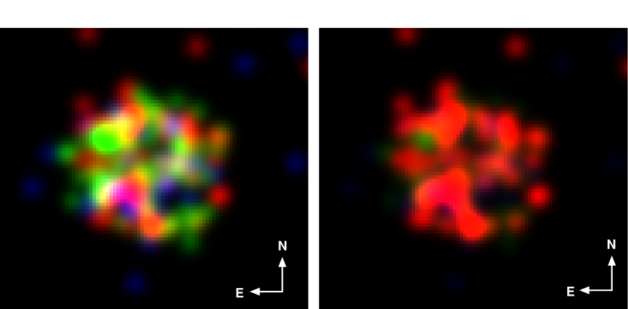
Figure 1: Left: Combined Chandra ACIS-I 0.3–7 keV image of r3-63. The colors represent different X-ray energy bands: 0.3–0.8 keV (red), 0.8–1.2 keV (green), and 1.2–7 keV (blue). The image is 22^′′ across. The softest band was multiplied by 1.4 to correct for decreasing sensitivity, but no correction for the Chandra response was performed on this image. Right: Same as left panel with each band exposure-corrected to show the true relative fluxes. This is the only resolved X-ray image of the SNR that fully corrects for the Chandra response as well as all time-variable changes in sensitivity.

We created X-ray three color images of the combined data, totaling 25 ks of exposure time. We used the energy bands 0.3–0.8 keV (red), 0.8–1.2 keV (green), and 1.2–7 keV (blue), producing an image in each band with a pixel scale of 0.246^′′ pixel^-1. These images were then smoothed with a Gaussian of $\sigma$=0.58^′′ and recombined into the color images shown in Figure 1. In these images, the SNR has a diameter of $\sim$11^′′ and 164 background-subtracted counts for a mean surface brightness of $\sim$4.5$\times$10^-16 erg cm^-2 s^-1 arcsec^-2 (0.3–7 keV).

The left panel shows the resulting image after the soft-band image was multiplied by 1.4 to correct for the $\sim$40% loss in sensitivity of Chandra at 0.5 keV observed between launch and 2002. This correction factor did not qualitatively change the image. The left panel of Figure 1 shows our 25 ks image of r3-63 without correcting for the Chandra response. Therefore it can be directly compared to the single-exposure (5 ks) image in K02 which also shows the Chandra detected counts without calibrating each band for the Chandra response. The difference between the left panel of Figure 1 and Figure 1 of K02 is that our figure contains 25 ks of exposure and that of K02 contains only 5 ks of exposure. The green color is due to the high sensitivity of Chandra at 1 keV.

The right panel shows the resulting image after normalizing each band by the effective exposure in that bandpass. We created the exposure maps for each bandpass and normalized the images using the CIAO script merge_all. The exposure maps correct for the lower sensitivity of Chandra at soft energies as well as the effects of the optical blocking filer (OBF) contamination, which has been building up since launch, decreasing the sensitivity at energies below 1 keV. Therefore this image is a better representation of the “true” X-ray color of the SNR.

We created lightcurves for 3^′′ aperture radii centered on 20000 randomly chosen positions in the SNR. These were measured with the CIAO task lightcurve using the counts from each of the five 5 ks observations to measure the corresponding errors from the merged event list. To be sure our errors were not underestimated because of the small number of counts ($\;\buildrel<\over{\sim}\;$20 ct bin^-1) in these lightcurves, we applied Poisson errors for the count rates. The use of Poisson errors, which are systematically larger than Gaussian ($\sqrt{N}$) errors, makes any detection of deviations from a constant count rate more reliable.

We also created a lightcurve for the SNR as a whole. This lightcurve had $>$20 ct bin^-1, allowing us to use Gaussian errors.

All of the lightcurves were fit to a constant count rate that produced the minimum value of $\chi^{2}$, in order to test for variability across observations. We also ran Monte Carlo simulations to test the reliability of the $\chi^{2}$ statistics when applied to these data.

Finally, we obtained the deepest Chandra ACIS-S observation (Observation ID 1575; 37.7 ks) available in the archive. Source r3-63 was not resolved in these data, but they contained $\sim$270 counts from the SNR. We extracted the spectrum using the CIAO script psextract, and we fit the spectrum with several model combinations using CIAO 3.2/Sherpa. Results are discussed as in §3.1.

3 Results

3.1 XMM-Newton

We present the 0.3–2.0 keV combined EPIC lightcurves of r3-63 from the 2002 and 2004 XMM-Newton observations in Fig. 2. The lightcurves are averaged over 200 s bins. The lightcurves of each observation are featureless but exhibit variability at high confidence. For example the lightcurve from the 2002 observation has $\chi^{2}/\nu=517/304$ when fitted to a constant count rate.

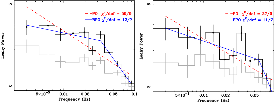
Figure 3: Dark histograms with error bars show the power density spectra (PDSs) of r3-63 from all of the 2002 XMM-Newton data (left) and from the xmm2 (see Table 1) 2004 data (right). Light histograms with error bars show the PDSs of the background in each observation. The PDSs are log-scaled and Leahy-normalized so that Poisson noise has a power of 2. The PDSs are averaged over many 333 s intervals with 5.2 s binning (64 bins per interval), and grouped. Dashed lines show the best fitting single power-law function. Solid lines show the best-fitting broken power-law function. Both PDSs are clearly described by broken power laws, indicating disk accretion.

We accumulated PDSs for the 2002 lightcurve and the 2004 lightcurve from observation xmm2 (see Table 1). The other 2004 lightcurves were not further analyzed due to high background variability, so that the 2004 PDS contained 700 counts. The PDSs were integrated over many 333 s intervals with 5.2 s bins (64 bins per interval); the PDSs were Leahy normalized, so that Poisson noise had a power of 2. The 2002 data were averaged over 191 intervals and the 2004 data were averaged over 60. The resulting PDSs are presented in Figure 3 as dark histograms with error bars; the PDSs are log scaled and grouped. It is clear that neither PDS can be described by a simple power law, but both are well-fit by broken power laws, indicating disk accretion (van der Klis, 1994; Barnard et al., 2003b, 2004a). These PDS features are not due to background fluctuations. The PDSs of the XMM-Newton background, shown with the light gray histograms in Figure 3, do not show the variability seen in the PDSs of r3-63.

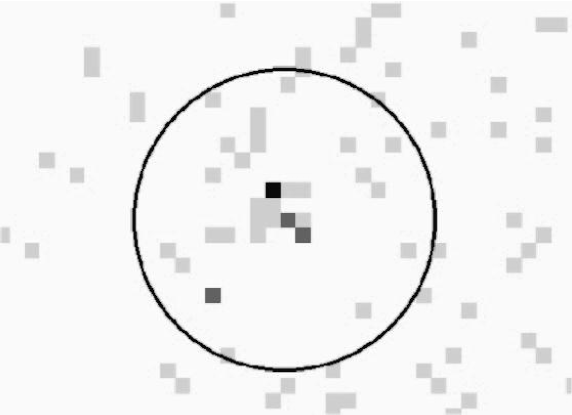
Figure 4: ACIS-I image of r3-63 from the 2004 July observation, taken during the program of XMM-Newton observations. In this observation r3-63 is too far off-axis to be resolved. The circle has a radius of 30^′′, indicating the XMM-Newton extraction region.

We show in Figure 4 the 2004 July ACIS-I image of r3-63; the circle indicates the 30^′′ extraction region used in our XMM-Newton observations. There is no clear source for the observed PDS within the 30^′′ apart from the SNR. Hence we conclude that the accreting object is coincident with the SNR itself.

We modeled the EPIC-pn spectra of r3-63 from the 2002 and 2004 observations with XSPEC 11.3.1. All of the spectral fits from both years were consistent. Therefore we focus on the results from the 2002 January observation, which had the highest number of counts.

The 2002 January spectrum was grouped to ensure $>$20 count bin^-1, and all counts outside the range 0.3–10 keV were discarded, as the instrument response is not well known outside this range. We found the useful range to be 0.3–2.1 keV. Following K02, we applied Raymond-Smith (RS) and non-equilibrium ionization (NEI) plasma models, first fixing the abundance to Solar, then allowing it to vary. We present the best fit models in Table 2. Fixed abundance values are provided in the table without any associated errors. Using previous knowledge about the SNR, we were able to limit the number of free parameters and find evidence in the spectrum for the presence of an LMXB in the SNR.

Like K02, the best-fitting model was an RS model with the O, Ne, and Fe abundances free to vary. All parameters of this fit are consistent with the K02 results within the quoted error ranges. However, this fit has 6 free parameters in a 16 parameter model, and we could find good fits by freeing almost any 6 of the parameters. The NEI fits with fixed abundances had slightly better fits than the RS fits with fixed abundances, but the NEI model has an additional free parameter in the ionization timescale ($\log n_{\rm e}t$).

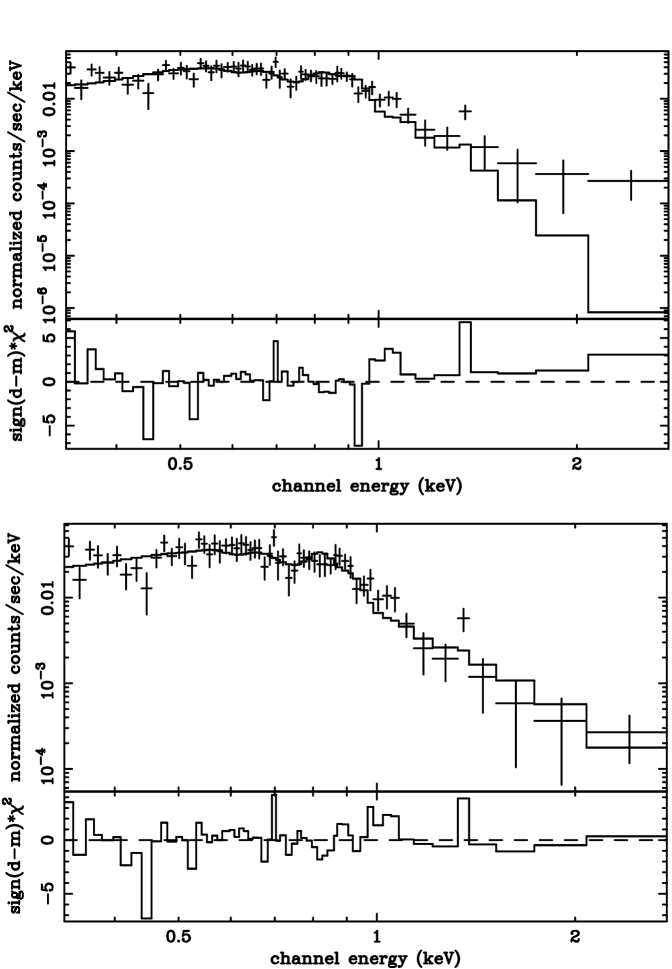
Figure 5: Top: Best fit Raymond-Smith model to the 0.3–2.1 keV EPIC-pn spectrum from the 2002 observation of r3-63 with abundances fixed to the values measured by Blair et al. (1982). The axes are log-scaled, and the spectrum is folded. The residuals to the fit are plotted beneath the spectrum, showing a slight hard excess. Bottom: Same as top, but with a power-law component added to the model. The hard excess is no longer present.

Most meaningful is the RS fit shown in the top panel of Figure 5, which had the abundances fixed to the values measured from optical spectra (${{\rm N}\over{\rm H}}=0.75({{\rm N}\over{\rm H}})_{\odot},{{\rm O}\over{\rm H}}=0.27({{\rm O}\over{\rm H}})_{\odot}$, and ${{\rm S}\over{\rm H}}=0.44({{\rm S}\over{\rm H}})_{\odot}$; Blair et al., 1982). This RS fit was much better than the one that assumed solar abundances, with the same number of free parameters. Additionally, this fit yielded the same temperature as K02, and like K02, this model fit had high $\chi^{2}/\nu$ (83/57).

The poor quality of the single-component spectral fits may be due to the presence of a second component in the spectrum. The spectrum of r3-63 is dominated by the SNR, but all of the single-component fits to the spectrum resulted in a slight hard excess, possibly due to a second emission component. The hard excess was also seen in the 2004 data. When the 2004 spectra were fitted with a RS model with abundances fixed to the values measured from optical spectra, the parameters were consistent with those from the fit to the 2002 observation, and as shown in Figure 6, the fit resulted in a hard excess. In addition, the inability to achieve a good fit to the 2002 data with the abundances fixed to the known values suggests that another emission component may be contaminating the spectral lines with continuum emission.

The spectral properties hint that the disk-accreting object detected in the PDSs could be producing a hard-excess and enhancing the continuum. We therefore added a power-law component to the absorbed RS and NEI models with the abundances fixed to the optical values. The results are detailed in Table 3; both cases show the presence of a soft power-law component. The NEI plus power-law model has a slightly better fit again because of the extra free parameter. The fit for the RS plus power-law model is shown in the bottom panel of Figure 5; there is no longer a hard excess in the residuals to the fit. This fit had $\chi^{2}/dof$ = 66/55, with the power-law contributing 26${}_{-16}^{+30}$% of the X-ray luminosity. According to an $F$-test, the power-law component is present with 0.998 significance.

The quality of the two-component fits was not as good as that of the fit from the RS model with the abundances free to vary. However, the two-component models use the known abundances and our knowledge that there is a variable source within the SNR, making these models more meaningful in the context of our knowledge about r3-63. The power-law component is much softer than typical pulsars or HMXBs which have photon indexes $\;\buildrel<\over{\sim}\;$1. The results of the two-component spectral fits are therefore more consistent with a power-law component coming from the accretion disk of a low accretion rate LMXB, supporting what is seen in the PDS.

The spectral data do not rule out a second component that is thermal in nature. We note that the hard excess can be equally well-fitted with the addition of a blackbody component with kT$\sim$0.2 keV. If the second component is thermal, it could be from the SNR itself. From the current data we cannot distinguish between the possibility that the second component in the spectrum is from the SNR or from an associated XRB. Therefore, the spectrum does not provide conclusive evidence for the presence of an XRB. However, the variability properties show that there is a variable source (i.e. an XRB) contributing to the data, and both the Chandra (see § 3.2) and XMM-Newton spectra of r3-63 are consistent with the presence of an XRB. These results suggest that the second component in the spectrum is from the XRB.

3.2 Chandra

We examined the PDS and energy spectrum of the deepest available Chandra observation of r3-63 to test their consistency with the XMM-Newton results. In addition we studied the 5 Chandra observations that resolve the SNR into a shell. The data were sufficient to find a region within the SNR that is likely to be variable. Considering the results from the XMM-Newton data, this region is likely the location of an associated X-ray binary.

We attempted to confirm the short term variability seen in the XMM-Newton data using the deepest Chandra observation of the region available in the archive. This observation was the 37.7 ks ACIS-S observation (Observation ID 1575). While r3-63 was not resolved in this observation, the 270 background-subtracted counts from r3-63 could be used to test for variability. However, the PDS was featureless. The 270 counts proved to be too few to detect the variability seen with XMM-Newton. This non-detection was not a surprise, as the quality of the detection clearly depends strongly on the number of counts in the observation. This effect is noticeable in the strength of the detections in the two XMM-Newton data sets. The variability detection is stronger in the 2002 PDS with 2200 counts than in the 2004 PDS with 700 counts (see Figure 3).

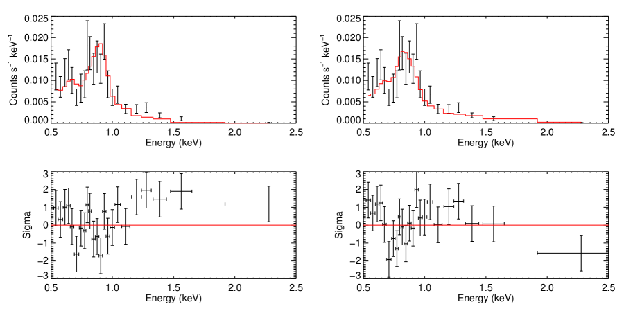
Figure 7: Top left: Best fit Raymond-Smith model to the 0.5–2.5 keV ACIS-S spectrum from the 37.7 ks observation of r3-63 with abundances fixed to the values measured by Blair et al. (1982). The model is shown with the histogram, and the data are shown with the error bars. This fit had 3 free parameters: the normalization, the temperature, and the absorption. Bottom left: The residuals to the fit are plotted beneath the spectrum, showing a slight hard excess. Top right: Same as top left, but with a power-law component added to the model. The abundances were fixed to the values measured by Blair et al. (1982). The absorption, temperature, and photon index were fixed to the values measured from the EPIC-pn spectrum, leaving the 2 normalization values as the only free parameters. Bottom right: The residuals to the fit are plotted beneath the spectrum. The hard excess is no longer present, consistent with the XMM-Newton result.

The second spectral component, which appears in the 2002 and 2004 XMM-Newton spectra, is not inconsistent with the Chandra spectral results from K02 or the lack of a variability detection in the K02 Chandra data. Such a component helps to explain the poor spectral fits in K02 when the abundances measured from optical spectra were applied. In addition, the best-fitting model in K02 was not consistent with the hardest spectral bin (see Figure 2 of K02), hinting at the presence of a hard excess. Finally, we refit the Chandra spectrum (ObsID 1575) between 0.5–2.5 keV with a two-component model, fixing the abundances, temperature, and photon index to the values determined using the XMM-Newton data. The result was a good fit, with $\chi^{2}/\nu=24.1/21$. This fit had only 2 free parameters: the normalization values of the 2 models. A single component RS model fit with the same fixed abundances but with $kT$ and $N_{H}$ free to vary (more free parameters than our 2 component fit) over the same energy range does not fit the data as well, with $\chi^{2}/\nu=27.5/20$. These fits are shown in Figure 7. The single-component fit clearly shows a hard excess that is well-fitted by the addition of the power-law component, consistent with the XMM-Newton results. Furthermore, the two-component fit to the Chandra spectrum indicates only 8% of the flux came from the second component. Therefore only $\sim$20 of the counts in these data are likely to be from the XRB, explaining the lack of a variability detection in this observation.

Figure 1 shows the combination of all resolved Chandra ACIS-I images of r3-63 we found in the data archive. Direct comparisons can be made between the left panel and K02 as the bands chosen to represent each color are the same for both images; however, it is important to note that the sensitivity of ACIS to soft ($\;\buildrel<\over{\sim}\;$1 keV) X-rays decreased by $\sim$15% over the 9 month baseline of these observations due to the build-up of contamination on the OBF. Only the panel on the right of Figure 1 shows the image fully corrected for the Chandra response, including the time-dependent loss of sensitivity to soft X-rays.

The added depth in the left panel of Figure 1 reveals some structure not easily seen in the 5 ks image from K02. The overall shell structure of the SNR is similar in both images, but the western lobes of the shell are more apparent in the combined image. The added depth shows fairly strong 0.8–1.2 keV emission in the western half of the SNR. In addition, the K02 image appeared strongly red (0.3–0.8 keV) on the north rim of the shell, the combined image has only small pockets of red on the north rim. The rest of the SNR appears to exhibit very similar colors to the K02 image, and the soft-band portion of our deeper image was corrected for decreased sensitivity. Therefore the greener north rim appears attributable to the increase in depth rather than to the decrease in sensitivity to soft ($<$1 keV) X-rays over the course of the observations.

The exposure-corrected image (right panel of Figure 1) shows the true relative X-ray fluxes of the different bands. It is clearly dominated by soft emission, consistent with the SNR spectrum.

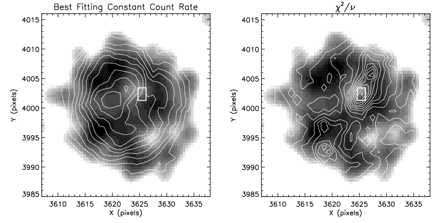
Figure 8: Left: Contours of the count rate as a function of aperture center position from the $\chi^{2}$ lightcurve analysis are overplotted on the X-ray image of the SNR. Contours are spaced at intervals of 0.0002 ct s^-1 and cover the range 0.0006–0.0024 ct s^-1. A white box marks the location of the center of all apertures with mean count rates $>$0.0015 ct s^-1 and $\chi^{2}_{\nu}>$1.945. Right: Contours of the best-fitting $\chi^{2}_{\nu}$ value as a function of aperture center position from the $\chi^{2}$ lightcurve analysis are overplotted on the same X-ray image. Contours are evenly spaced at intervals of 0.2 and cover the range 0$\leq\chi^{2}_{\nu}\leq 2.2$. Notice the area of high $\chi^{2}_{\nu}$ in the northwest quadrant of the SNR. The white box marks the same location as in the left panel.

More intriguing are the results of the variability analysis. The SNR sampled as a whole was well-fitted ($\chi^{2}_{\nu}=0.8$) by a constant count rate of 0.0067 ct s^-1; however when the SNR was broken into smaller regions, the lightcurves of regions northwest of the center showed evidence for variability. These results are shown in the right panel of Figure 8 with contours of the $\chi^{2}_{\nu}$ values for fits to a constant count rate overplotted on the greyscale Chandra X-ray image of the SNR. There is a noticeable area of high $\chi^{2}_{\nu}$ values in the northwest quadrant of the SNR, suggesting that if any portion of the SNR varied over the course of the observations, it was this portion.

For comparison, contours of the best-fitting constant rates are shown overplotted on the same greyscale image in the left panel of Figure 8. The contours in this panel show the effects of our aperture size, which effectively re-samples the data to 6^′′ spatial resolution resulting in the loss of most of the structure seen at full resolution. The only detail that survives the re-sampling is the off-center peak in emission indicating that the eastern half of the SNR is brighter than the western half.

We determined the threshold for variability detection in our low-count lightcurves. With the 4 degrees of freedom offered by our 5-point lightcurves, a $\chi^{2}_{\nu}$ value of 1.945 corresponds to a 90% probability for variability in the lightcurve. We ran Monte Carlo simulations drawing 5 random lightcurve points with 3–19 counts in each. This range of counts represented the range seen in the lightcurves from our data. We then applied Poisson errors and computed $\chi^{2}_{\nu}$ in the same fashion as applied to our data. In 10⁴ simulations, 87% of the lightcurves had $\chi^{2}_{\nu}<1.945$, similar to the prediction of 90% from $\chi^{2}$ statistics.

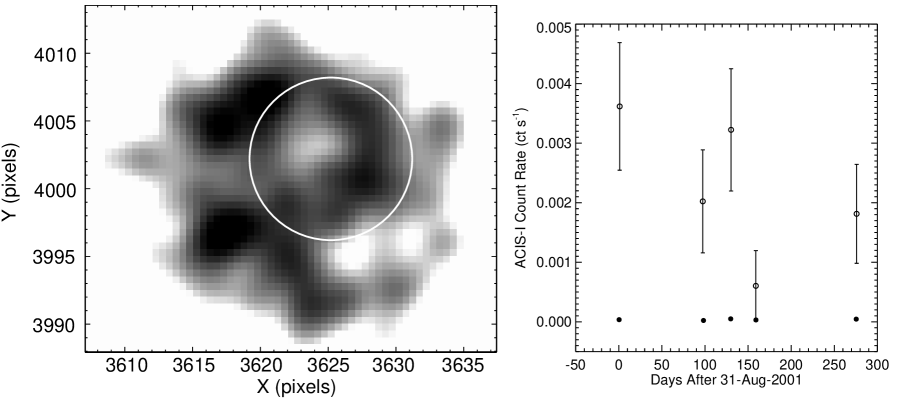
Figure 10: Left: Smoothed 0.3–7 keV image of r3-63. Darker areas denote higher X-ray flux. The white circle shows the 6 pixel aperture centered on the most variable portion of the SNR. Right: The lightcurve of the aperture shown is marked with the open circles. This lightcurve has a best-fitting constant rate of 0.0018 ct s^-1, and $\chi^{2}/{\nu}$=9/4, which has 94% probability of variability. Filled circles mark the lightcurve for the background scaled to an equivalent area. The points are larger than the errors in the background count rates.

We also created a lightcurve of the background in our combined r3-63 image with an extraction area of 0.34 arcmin² so that the number of counts per bin were $\sim$10. Poisson errors were used. This lightcurve had $\chi^{2}_{\nu}=0.38$ when fitted to a constant rate, clearly indicating that the background was not responsible for any variability seen in the r3-63 lightcurves. In addition, the mean background count rate in a 3^′′ radius aperture was just 2% of the rate observed in apertures of identical size in r3-63, further eliminating the background as a source of variability in our lightcurves. The background lightcurve is shown with that of the variable region in Figure 10.

We determined the location of the most variable region in the SNR. The mean position of all aperture centers with $\chi^{2}_{\nu}>1.945$ and best-fit count rates $>$0.0015 ct s^-1 was $X=3625.2\pm 0.6,Y=4002.2\pm 0.9$. This location is marked with a white box on Figure 8. The corresponding R.A. and DEC. are 00:43:27.81$\pm$0.3^′′ (0.030^s), 41:18:31.2$\pm$0.4^′′ (J2000). The location of this centroid shows that the elongation of the variable region toward the outer portion of the SNR (northwest of the centroid) is due to very low count rates in those outermost apertures.

We investigated the impact of the most variable region on the $\chi^{2}_{\nu}$ distribution. The left panel of Figure 9 shows a histogram of the $\chi^{2}_{\nu}$ values measured for the lightcurves of all aperture centers with count rates $>$0.0015. The distribution falls off quite smoothly to $\chi^{2}_{\nu}$=1.5; then there appears to be some excess trials with $\chi^{2}_{\nu}>1.5$. The right panel shows the same histogram with all aperture centers in the region $X=3625.2\pm 1.2,Y=4002.2\pm 1.8$ removed. The excess at high $\chi^{2}_{\nu}$ disappears, providing further assurance that this region of the SNR is the most likely to be variable.

An aperture at the most variable position in the SNR and the corresponding lightcurve are shown in Figure 10. The lightcurve has $\chi^{2}/{\nu}$=9/4, which is a detection of variability with 94% confidence according to standard $\chi^{2}$ statistics. We checked this reliability with Monte Carlo simulations performed as described above. In 10⁴ simulations, 94% had $\chi^{2}/{\nu}<$9/4, as expected from $\chi^{2}$ statistics.

The poor fits to a constant count rate seen in the northwest portion of the SNR do not provide a highly reliable detection of variability, as the high $\chi^{2}/{\nu}$ value is clearly due to only one outlying data point with a low count rate. Furthermore, in order to isolate this variability in the Chandra data, we have eliminated about 75% of the SNR flux. On the other hand, considering the XMM-Newton data, which show that the SNR contains an XRB, this region is the most likely location of an XRB that can be found with currently-available data. Further on-axis Chandra observations will be required to ascertain this possible detection.

Additional concern regarding the variability of this region of the SNR is warranted because it contains some soft (0.3–0.8 keV) emission and the lightcurve shows a decrease in flux over the 9-month baseline of the observations. The build-up of contamination on the OBF surely contributed somewhat to this decrease in count rate (see § 2.2); however, the level of variability observed cannot be explained by OBF contamination effects. The effect of the contamination was $\sim$40% loss of sensitivity at 0.5 keV from April 2000 to June 2002. Therefore, assuming the decrease was linear with time, during the 9 months between the first and last resolved observation of r3-63, the sensitivity dropped by $\sim$15% at 0.5 keV. We tested the effects of this decrease in sensitivity by artificially lowering the count rates of our Monte Carlo simulations by 0–20%, increasing by 4% at each consecutive artificial data point. The simulations still showed at least 94% of the artificial lightcurves had $\chi^{2}/{\nu}<$9/4 when fitted to a constant rate. The variability does not appear to be due to the effects of the OBF contamination.

The SNR center is $X=3623.5\pm 1.0,Y=3999.9\pm 1.0$ (00:43:27.88$\pm$0.5^′′ (0.04^s), 41:18:30.1$\pm$0.5^′′). The most variable position in the SNR is therefore 0.8${}^{\prime\prime}\pm 0.6^{\prime\prime}$ west and 1.1${}^{\prime\prime}\pm 0.7^{\prime\prime}$ north of the SNR center, 1.4${}^{\prime\prime}\pm 0.9^{\prime\prime}$ distant from the SNR center. This location provides additional evidence that the XRB is associated with the SNR, and it constrains the velocity of the XRB with respect to the SNR center.

The probable location of the XRB makes it likely to be associated with the SNR. The mean density of point sources with 0.3–7 keV luminosities $>2\times 10^{35}$ erg s^-1 is 0.4 sources arcmin^-2 in the area from 7.5^′ to 8.5^′ from the center of M31, according to a search of the Kong et al. (2002b) catalog. Using this value as the density of sources at the galactocentric distance of r3-63 (8.5^′), the probability of an unassociated X-ray source falling inside the 5.5^′′ radius of the SNR is 1%. The probability decreases to 0.1% for an unassociated source to fall within 2^′′ of the SNR center.

Because an XRB at the variable position in the SNR was likely created by the SN event, we can use the distance of the XRB from the SNR center along with the SNR age to constrain the projected velocity of the XRB. Assuming a distance of 780 kpc to M31 (Williams, 2003), this separation corresponds to a projected distance of 5.3$\pm$3.4 pc. Taking the SNR age to be 21${}^{+1}_{-5}$ kyr, from the best-fitting spectral parameters of K02, the projected velocity of the binary system with respect to the SNR center is 240${}^{+280}_{-160}$ km s^-1.

4 Discussion: HMXB or LMXB?

There is no foolproof method for determining whether the variable source in r3-63 is a HMXB or LMXB from the currently-available data. We therefore use the clues available to make an indirect argument that the source is a LMXB. This indirect argument is based on available optical images, X-ray images, spectra, PDSs, and lightcurves. We then investigate the possibility of the existence of a SNR/LMXB association in r3-63 based on the properties of LMXBs and current models of LMXB formation from SNe.

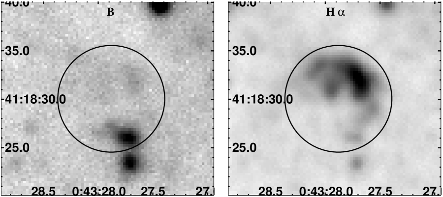
Figure 11: Left: The Local Group Survey $B$-band image of r3-63. The image shows the same patch of sky shown by the X-ray image in Figure 1 down to $B\sim 21$. The black circle shows the 11^′′ diameter of the SNR shell, revealing one bright star ($B\sim 19.4$) in the shell 5^′′ southwest of the SNR center. Right: The Local Group Survey H$\alpha$ image of r3-63 is shown for comparison to the broadband image so that the relative positions of continuum sources and the SNR shell can be compared.

The optical counterpart search of Williams et al. (2004) using the data of the Local Group Survey (LGS; Massey et al., 2001) revealed no stellar counterpart to r3-63 down to $V=20.6$. Broadening the search of these data to include the full diameter of the SNR (see Figure 11, left panel) reveals a bright star within the shell region. The circles on the LGS $B$-band and H$\alpha$ images in Figure 11 mark the 11^′′ diameter shell of the SNR. The H$\alpha$ image is shown here only to facilitate comparisons between the locations of the optical shell and continuum sources in the region. There is a $B$=19.4 (M${}_{B}\sim-5.4$ at distance and typical extinction to M31) star near the southwest edge of the shell. This star is 5^′′ (19 pc) from the SNR center. If this star is a HMXB, it is unlikely associated with the SNR, as any kick that would move the binary 19 pc in 20 kyr (900 km s^-1) would disrupt the binary.

No bright star ($B<21$) is seen in the northwest portion of the SNR. Therefore, if the X-ray variability seen in the Chandra data is real, then the XRB that caused it is not a bright HMXB with a companion earlier than B1 (M${}_{B}<-4$). On the other hand, the optical data still allow an HMXB with a later B star secondary, and if the probable variability seen in the Chandra data is not real, there could be an unassociated bright HMXB in the SNR. Since there are few known HMXBs in M31 (Williams et al., 2004), such a coincidence is unlikely. We therefore conclude that the available optical data do not yield evidence to support the idea that the XRB in r3-63 is an HMXB, but they do not completely rule out the possibility.

In addition, most young HMXBs are Be/X-ray systems that contain pulsars (Liu et al., 2000). These HMXBs typically have hard X-ray spectra. The power-law component of the spectrum of r3-63 is soft. Furthermore, the PDSs of pulsars are dominated by pulsations. The lack of a peak in the PDS of r3-63 (see Figure 3) indicates the variability is not dominated by pulsations. These data do not rule out the possibility that a pulsar could be present, but they provide no evidence for the presence of pulsations or a HMXB. We therefore suggest the SNR contains an associated LMXB because of (1) the appearance of the region in optical images, (2) the appearance of the XMM-Newton extraction region in the resolved contemporaneous Chandra data, (3) the variability seen in the Chandra resolved lightcurves, (4) the softness of the X-ray spectrum, and (5) the properties of the XMM-Newton PDS.

A LMXB in r3-63 is reasonable considering the properties of known LMXB systems and models of LMXB formation and evolution. The probable position of the XRB is consistent with current systemic and kick velocity distributions, and LMXB formation models allow for the possibility that X-ray activity could begin in an LMXB shortly after the SN event.

The more central portion of the variable region in r3-63 (discussed in § 3.2) provides the most reasonable velocity of the binary away from the SNR center ($\sim$100 km s^-1). Several Galactic black hole binaries have projected orbital velocities of $>$100 km s^-1 (see values in Orosz, 2003), suggesting binary systems can survive such a kick velocity. In addition, Kalogera et al. (1998) show that LMXBs can survive in simulations with mean kick velocities of 100–200 km s^-1, and Fryer et al. (1998) show that for a double-peaked kick velocity distribution, some binaries survive kicks in the low velocity peak. Such a double-peak is seen in the velocity distribution of pulsars, with a low velocity peak at 90 km s^-1 (Arzoumanian et al., 2002), and kicks from asymmetric SNe could produce such velocities (Scheck et al., 2004; Fryer, 2004). Finally, the low end of our allowed velocity range for the XRB in r3-63 overlaps the results of earlier simulations of the systemic velocities of binary systems that survive a SN event to become LMXBs (180$\pm$80 km s^-1, Brandt & Podsiadlowski, 1995).

A SNR/LMXB association would be the first of its kind, but such objects may be extremely rare because SNRs fade quickly and a surviving binary could take some time to become X-ray active. From a theoretical point of view, both HMXBs and LMXBs form from SNe, and since many examples of both types of systems are known in our Galaxy, some of these systems clearly survive the SN event.

Survival of a SN is easier if the secondary star is massive. In spherically symmetric explosions, i.e. those without a kick, the binary will become unbound if more than 50% of the pre-SN mass is ejected. This 50% criterion is more likely to be met in low mass systems. If the SN provides a kick, this rule no longer holds, but for small to intermediate kick velocities the survival probability still increases with companion mass (Kalogera, 1996).

While it is true that the parameter space for the formation of neutron star LMXBs is very small (King & Kolb, 1997; Kalogera et al., 1998; Kalogera & Webbink, 1998), many LMXBs must survive their birth SNe to create the known population. In addition, many LMXBs are transient sources, suggesting that there may be a large, dormant, as yet undiscovered population which would add to the SN survival rate. This possibility that many low-mass binaries survive SNe is confirmed by some evolutionary calculations, in which LMXBs form for a wide range of kick velocities (e.g. Brandt & Podsiadlowski, 1995; Kalogera et al., 1998).

After the SN event, most systems must evolve into Roche-lobe contact before mass transfer, and hence X-ray activity, starts. For the onset of mass-transfer to occur within $\sim$20 kyr of the SN requires the system to have emerged from the SN almost semi-detached, while avoiding a merger in the immediate eccentric post-SN orbit. The potential for low-mass systems not to evolve into LMXBs until after the SNR fades, coupled with the fact that the systemic velocities of HMXBs are on average smaller than those of LMXBs, would favor the appearance of a HMXB inside its parent SNR over that of a LMXB.

Even though HMXBs may be more likely to survive a SN and begin active accretion while their parent remnant is still bright, very few SNR/HMXB associations are known (see § 1). If the conditions necessary to produce a SNR/LMXB association are even less likely, as suggested by the formation simulations and timescale arguments, SNR/LMXB associations would certainly be rare, but they could exist.

5 Conclusions

We have studied in detail the timing analysis of the X-ray emission from the M31 SNR r3-63 using both XMM-Newton and Chandra. The XMM-Newton data provide PDSs which show variability within the SNR lightcurve at very high confidence. We can associate Type A variability with the SNR, indicating disk accretion and probable Roche lobe overflow. The accreting object is most likely a neutron star or black hole in a binary system. These data therefore contain the signature of an accreting X-ray binary very close to the SNR, presumably formed by the SN event. If Roche lobe overflow is responsible for the mass transfer, the binary is likely a LMXB, which would make r3-63 the first SNR known that contains a LMXB.

Although deeper resolved optical and X-ray data are required to confirm the lack of a HMXB near the center of r3-63, we see no clear evidence for a HMXB in the currently-available data. On the other hand, the data are all consistent with an associated LMXB in r3-63. If we have found the first SNR/LMXB association, we have had to search outside the Galaxy within the largest spiral in the Local Group to find it. Confirmation of the associated LMXB would support the idea that such associations are rare, but would also show that LMXBs can start mass-transfer very shortly after the formation of the compact object.

Detailed analysis of the spatially-resolved lightcurve from all resolved detections of r3-63 in the Chandra archive suggest that, while the SNR taken as a whole is not significantly variable, there is variability detected at the 94% confidence level 1.4${}^{\prime\prime}\pm$0.9^′′ northwest of the SNR center which cannot be attributed entirely to ACIS contamination issues or photometric errors. Further observations are needed to confirm the variability, determine a more precise SNR age, and directly measure the position of the XRB.

The current age estimate of the SNR and XRB, along with the possible XRB position, provide an estimate of the projected systemic velocity away from the SNR center. If the variability seen in the Chandra data is real and marks the location of the XRB detected by XMM-Newton, then the XRB associated with the SNR is 5.3$\pm$3.4 pc (projected distance) from the SNR center. With a SNR age of 21${}^{+1}_{-5}$ kyr (K02), this separation corresponds to an XRB velocity estimate of 240${}^{+280}_{-160}$ km s^-1 with respect to the SNR center. The low end of this range is reasonable given current knowledge of the distribution of neutron star and black hole velocities (Arzoumanian et al., 2002; Orosz, 2003), the expected kick velocities from asymmetric SNe (Scheck et al., 2004; Fryer, 2004), and the results of simulations of binary survival of SN kicks (Brandt & Podsiadlowski, 1995; Kalogera et al., 1998). On the other hand, the system could not have remained bound and acquired a systemic velocity close to the high end of this range.

Presently, r3-63 appears to be an excellent candidate SNR/LMXB system. The broken power law PDS, the soft X-ray spectrum, the non-detection of pulsations, and the lack of bright stars near the probable XRB position all support the idea that r3-63 contains a LMXB. Such systems must be very rare, possibly due to the supernova survival rate of low mass binary systems and/or the timing necessary for a low-mass system to begin mass-transfer while its birth SNR is still bright. More direct evidence is needed to confirm this association and determine if SNR/LMXB systems exist.

Support for this work was provided by NASA through grant number GO-9087 from the Space Telescope Science Institute and through grant number GO-3103X from the Chandra X-Ray Center. MRG acknowledges support from NASA LTSA grant NAG5-10889. RB was funded by PPARC.

Table 1: Observations used for the study.

ObsID	Date	R.A. (J2000)	Dec. (J2000)	Roll (deg.)	Exp. (ks)	Sep. (′)
1577	2001 Aug 31	00 43 07.3	41 19 17.7	143.0	4.9	4.0
2895	2001 Dec 07	00 43 05.4	41 17 33.6	271.7	4.9	4.4
2897	2002 Jan 08	00 43 09.9	41 18 43.8	292.4	4.9	3.4
2896	2002 Feb 06	00 43 06.0	41 16 47.2	309.5	4.9	4.4
2898	2002 Jun 02	00 43 10.5	41 19 16.4	88.6	4.9	3.3
xmm1	2002 Jan 06	00 42 39.1	41 15 47.0	250	64.5	9.8
xmm2	2004 Jul 16	00 42 42.1	41 16 57.2	64	20.3	8.7
xmm3	2004 Jul 18	00 42 42.3	41 16 58.2	63	21.9	8.7
xmm4	2004 Jul 19	00 42 42.2	41 16 57.2	63	27.1	8.7

Table 2: Results of fitting Raymond-Smith and non-equilibrium ionization plasma models to the 2002 January 6 XMM-Newton spectrum of r3-63. Uncertainties are quoted at a 90% confidence level for fits with $\chi^{2}$/dof $<$2. Fixed abundance values are given with no uncertainties.

	$N_{\rm H}$	k$T$	$\log$ $n_{\rm e}t$	N	O	Ne	S	Fe	$L_{0.3-10}$
Model	($\times 10^{21}$ cm-2)	(keV)							($\times$1037 erg s-1)	$\chi^{2}$/dof
RS	0.6	0.25	$\cdots$	1	1	1	1	1	0.7	122/57
	4.1${}^{+0.6}_{-0.7}$	0.143${}^{+0.008}_{-0.004}$	$\cdots$	0.75	0.27	1	0.44	1	1.52${}^{+0.14}_{-0.5}$	83/57
	0.7${}^{+1.8}_{-0.6}$	0.31${}^{+0.06}_{-0.08}$	$\cdots$	1	0.33${}^{+0.19}_{-0.12}$	0.51$\pm$0.22	1	0.13${}^{+0.08}_{-0.05}$	0.90$\pm$0.14	58/54
NEI	1.0${}^{+1.1}_{-0.7}$	1.3$\pm$0.7	10.1$\pm$0.2	1	1	1	1	1	0.8${}^{+0.2}_{-0.5}$	74/56
	2.6$\pm$0.8	0.186$\pm$0.012	13.5${}_{-0.3}^{+0.2}$	0.75	0.27	1	0.44	1	4.0$\pm$?	77/56

Table 3: Results of fitting Raymond-Smith and non-equilibrium ionization plasma models plus a power-law component to the 2002 January 6 XMM-Newton spectrum of r3-63. Abundances were fixed to values measured from Blair et al. (1982). Uncertainties are quoted at a 90% confidence level for fits with $\chi^{2}$/dof $<$2.

	$N_{\rm H}$	k$T$	$\log$ $n_{\rm e}t$	photon	$L_{0.3-10}$ (total)	$L_{0.3-10}$ (power-law)
Model	($\times 10^{21}$ cm-2)	(keV)		index	($\times$1037 erg s-1)	($\times$1037 erg s-1)	$\chi^{2}$/dof
RS	2.8${}^{+1.3}_{-0.9}$	$0.16\pm 0.02$	$\cdots$	$3.2\pm 1.5$	3.1${}^{+0.9}_{-0.4}$	$0.8_{-0.5}^{+0.9}$	66/55
NEI	2.3${}^{+0.7}_{-0.6}$	0.189${}^{+0.014}_{-0.013}$	13.69${}_{-0.18}^{+0.01}$	3.7${}^{+1.3}_{-1.6}$	2.5${}^{+0.8}_{-0.3}$	0.07${}^{+1.2}_{-0.07}$	61/54

Figure 2: Combined 0.3–2.0 keV XMM-Newton/EPIC lightcurves of r3-63 from the 2002 (top) and 2004 (bottom three) observations, binned to 200 s. The x- and y- axes are identical for all observations, to aid comparison.

Figure 6: Best fit Raymond-Smith model to the 0.3–2.5 keV EPIC-pn spectrum from the 2004 observation of r3-63 with abundances fixed to the values measured by Blair et al. (1982). The axes are log-scaled, and the spectrum is folded. The residuals to the fit are plotted beneath the spectrum, showing a hard excess consistent with that seen in the single-component fit to the 2002 data.

Figure 9: Left: Histogram the $\chi^{2}_{\nu}$ value vs. the number of random apertures with 6 pixel radius that result in a lightcurve with that value when fit to a constant count rate. All apertures with mean count rates $>$0.0015 count s^-1 are included. Right: Same as left panel with the results from all apertures with centers at $X=3625.5\pm 1.4,Y=4002.5\pm 1.8$, as well as those with mean count rates $<$0.0015 count s^-1, removed.

References

- Arzoumanian et al. (2002) Arzoumanian, Z., Chernoff, D. F., & Cordes, J. M. 2002, ApJ, 568, 289
- Barnard et al. (2003a) Barnard, R., Kolb, U., & Osborne, J. P. 2003a, A&A, 411, 553
- Barnard et al. (2004a) —. 2004a, A&A, 423, 147
- Barnard et al. (2003b) Barnard, R., Osborne, J. P., Kolb, U., & Borozdin, K. N. 2003b, A&A, 405, 505
- Barnard et al. (2004b) Barnard, R., Osborne, J. P., Kolb, U. C., & Haswell, C. A. 2004b, in Interacting Binaries: Accretion, Evolution and Outcomes, Eds. L. Angellini et al., astro-ph/0409122
- Blair et al. (1982) Blair, W. P., Kirshner, R. P., & Chevalier, R. A. 1982, ApJ, 254, 50
- Brandt & Podsiadlowski (1995) Brandt, N., & Podsiadlowski, P. 1995, MNRAS, 274, 461
- Braun (1990) Braun, R. 1990, ApJS, 72, 755
- Chu et al. (2000) Chu, Y., Kim, S., Points, S. D., Petre, R., & Snowden, S. L. 2000, AJ, 119, 2242
- Coe et al. (2000) Coe, M. J., Haigh, N. J., & Reig, P. 2000, MNRAS, 314, 290
- D’Odorico et al. (1980) D’Odorico, S., Dopita, M. A., & Benvenuti, P. 1980, A&AS, 40, 67
- Fryer et al. (1998) Fryer, C., Burrows, A., & Benz, W. 1998, ApJ, 496, 333
- Fryer (2004) Fryer, C. L. 2004, ApJ, 601, L175
- Gaensler et al. (2001) Gaensler, B. M., Pivovaroff, M. J., & Garmire, G. P. 2001, ApJ, 556, L107
- Geldzahler et al. (1980) Geldzahler, B. J., Pauls, T., & Salter, C. J. 1980, A&A, 84, 237
- Halpern et al. (2004) Halpern, J. P., Gotthelf, E. V., Camilo, F., Helfand, D. J., & Ransom, S. M. 2004, ApJ, 612, 398
- Hughes et al. (2001) Hughes, J. P., Slane, P. O., Burrows, D. N., Garmire, G., Nousek, J. A., Olbert, C. M., & Keohane, J. W. 2001, ApJ, 559, L153
- Kalogera (1996) Kalogera, V. 1996, ApJ, 471, 352
- Kalogera et al. (1998) Kalogera, V., Kolb, U., & King, A. R. 1998, ApJ, 504, 967
- Kalogera & Webbink (1998) Kalogera, V., & Webbink, R. F. 1998, ApJ, 493, 351
- King & Kolb (1997) King, A. R., & Kolb, U. 1997, ApJ, 481, 918
- Kong et al. (2002a) Kong, A. K. H., Garcia, M. R., Primini, F. A., & Murray, S. S. 2002a, ApJ, 580, L125
- Kong et al. (2002b) Kong, A. K. H., Garcia, M. R., Primini, F. A., Murray, S. S., Di Stefano, R., & McClintock, J. E. 2002b, ApJ, 577, 738
- Liu et al. (2000) Liu, Q. Z., van Paradijs, J., & van den Heuvel, E. P. J. 2000, A&AS, 147, 25
- Massey et al. (2001) Massey, P., Hodge, P. W., Holmes, S., Jacoby, G., King, N. L., Olsen, K., Saha, A., & Smith, C. 2001, in American Astronomical Society Meeting, Vol. 199, 13005+
- Orosz (2003) Orosz, J. A. 2003, in IAU Symposium, 365–+
- Roberts & Colbert (2003) Roberts, T. P., & Colbert, E. J. M. 2003, MNRAS, 341, L49
- Scheck et al. (2004) Scheck, L., Plewa, T., Janka, H.-T., Kifonidis, K., & Müller, E. 2004, Physical Review Letters, 92, 011103
- Strüder et al. (2001) Strüder, L., et al. 2001, A&A, 365, L18
- Turner et al. (2001) Turner, M. J. L., et al. 2001, A&A, 365, L27
- Uttley et al. (2002) Uttley, P., McHardy, I. M., & Papadakis, I. E. 2002, MNRAS, 332, 231
- van der Klis (1994) van der Klis, M. 1994, ApJS, 92, 511
- Williams (2003) Williams, B. F. 2003, AJ, 126, 1312
- Williams et al. (2004) Williams, B. F., Garcia, M. R., Kong, A. K. H., Primini, F. A., King, A. R., Di Stefano, R., & Murray, S. S. 2004, ApJ, 609, 735++