Star Formation in Isolated Disk Galaxies.
II. Schmidt Laws and Efficiency of Gravitational Collapse

Abstract

We model gravitational instability in a wide range of isolated disk galaxies, using GADGET, a three-dimensional, smoothed particle hydrodynamics code. The model galaxies include a dark matter halo and a disk of stars and isothermal gas. Absorbing sink particles are used to directly measure the mass of gravitationally collapsing gas. Below the density at which they are inserted, the collapsing gas is fully resolved. We make the assumption that stars and molecular gas form within the sink particle once it is created, and that the star formation rate is the gravitational collapse rate times a constant efficiency factor. In our models, the derived star formation rate declines exponentially with time, and radial profiles of atomic and molecular gas and star formation rate reproduce observed behavior. We derive from our models and discuss both the global and local Schmidt laws for star formation: power-law relations between surface densities of gas and star formation rate. The global Schmidt law observed in disk galaxies is quantitatively reproduced by our models. We find that the surface density of star formation rate directly correlates with the strength of local gravitational instability. The local Schmidt laws of individual galaxies in our models show clear evidence of star formation thresholds. The variations in both the slope and the normalization of the local Schmidt laws cover the observed range. The averaged values agree well with the observed average, and with the global law. Our results suggest that the non-linear development of gravitational instability determines the local and global Schmidt laws, and the star formation thresholds. We derive from our models the quantitative dependence of the global star formation efficiency on the initial gravitational instability of galaxies. The more unstable a galaxy is, the quicker and more efficiently its gas collapses gravitationally and forms stars.

1. INTRODUCTION

Stars form at widely varying rates in different disk galaxies (Kennicutt, 1998a). However, they appear to follow two simple empirical laws. The first is the correlation between the star formation rate (SFR) density and the gas density, the “Schmidt law” as first introduced by Schmidt (1959):

$$\Sigma_{\rm SFR}=A\ \Sigma_{\rm gas}^{\rm N}$$ (1)

where $\Sigma_{\rm SFR}$ and $\Sigma_{\rm gas}$ are the surface densities of SFR and gas, respectively.

When $\Sigma_{\rm gas}$ and $\Sigma_{\rm SFR}$ are averaged over the entire star forming region of a galaxy, they give rise to a global Schmidt law. Kennicutt (1998b) found a universal global star formation law in a large sample that includes 61 normal spiral galaxies that have $\rm H_{\alpha}$, H_I and CO measurements and 36 infrared-selected starburst galaxies. The observations show that both the slope $N\sim$ 1.3–1.5 and the normalization $A$ appear to be remarkably consistent from galaxy to galaxy. There are some variations, though. For example, Wong & Blitz (2002) reported $N\sim$ 1.1–1.7 for a sample of seven molecule-rich spiral galaxies, depending on the correction of the observed $\rm H_{\alpha}$ emission for extinction in deriving the star formation rate. Boissier et al. (2003) examined 16 spiral galaxies with published abundance gradients and found $N\sim$ 2.0. Gao & Solomon (2004a) surveyed HCN luminosity, a tracer of dense molecular gas, from 65 infrared or CO-bright galaxies including nearby normal spiral galaxies, luminous infrared galaxies, and ultraluminous infrared galaxies. Based on this survey, Gao & Solomon (2004b) suggested a shallower star formation law with a power-law index of 1.0 in terms of dense molecular gas content.

When $\Sigma_{\rm gas}$ and $\Sigma_{\rm SFR}$ are measured radially within a galaxy, a local Schmidt law can be measured. Wong & Blitz (2002) investigated the local Schmidt laws of individual galaxies in their sample. They found similar correlations in these galaxies but the normalizations and slopes vary from galaxy to galaxy, with $N\sim$ 1.2–2.1 for total gas, assuming that extinction depends on gas column density (or, $N\sim$ 0.8–1.4 if extinction is assumed constant). Heyer et al. (2004) reported that M33 has a much deeper slope, $N\simeq 3.3$.

The second empirical law is the star formation threshold. Stars are observed to form efficiently only above a critical gas surface density. Martin & Kennicutt (2001) studied a sample of 32 nearby spiral galaxies with well-measured $\rm{H_{\alpha}}$ and H₂ profiles, and demonstrated clear surface-density thresholds in the star formation laws in these galaxies. They found that the threshold gas density (measured at the outer threshold radius where SFR drops sharply) ranges from 0.7 to 40 $\rm{M_{\odot}\ pc^{-2}}$ among spiral galaxies, and the threshold density for molecular gas is $\sim$5–10 $\rm{M_{\odot}\ pc^{-2}}$. However, they found that the ratio of gas surface density at the threshold to the critical density for Toomre (1964) gravitational instability, $\alpha_{Q}=\Sigma_{\rm gas}/\Sigma_{\rm crit}$, is remarkably uniform with $\alpha_{Q}=0.69\pm 0.2$. They assumed a constant velocity dispersion of the gas, the effective sound speed, of $c_{s}=6$ km s^-1. Such a density threshold applies to normal disk galaxies (e.g., Boissier et al. 2003), elliptical galaxies (e.g., Vader & Vigroux 1991), low surface brightness galaxies (van der Hulst et al., 1993), and starburst galaxies (Elmegreen, 1994). However, there are a few exceptions, such as dwarf and irregular galaxies (e.g., Hunter, Elmegreen & Baker 1998). Furthermore, inefficient star formation can be found well outside the threshold radius (Ferguson et al., 1998).

What is the origin of the Schmidt laws and the star formation thresholds? The mechanisms that control star formation in galaxies, such as gravitational instability, supersonic turbulence, magnetic fields, and rotational shear are widely debated (Shu et al. 1987; Elmegreen 2002; Larson 2003; Mac Low & Klessen 2004). At least four types of models are currently discussed. The first type emphasizes self-gravity of the galactic disk (e.g., Quirk 1972; Larson 1988; Kennicutt 1989; Elmegreen 1994; Kennicutt 1998b). In these models, the Schmidt laws do not depend on the local star formation process, but are simply the results of global gravitational collapse on a free-fall time. In the second type, the global star formation rate scales with either the local dynamical time, invoking cloud-cloud collisions (e.g. Wyse 1986; Wyse & Silk 1987; Silk 1997; Tan 2000), or the local orbital time of the galactic disk (e.g. Elmegreen 1997; Hunter et al. 1998). A third type, which invokes hierarchical star formation triggered by turbulence, has been proposed by Elmegreen (2002). In this model, the Schmidt law is scale-free, and the star formation rate depends on the probability distribution function (PDF) of the gas density produced by galactic turbulence, which appears to be log-normal in simulations of turbulent molecular clouds and interstellar medium (e.g., Scalo et al. 1998; Passot & Vázquez-Semadeni 1998; Ostriker, Gammie, & Stone 1999; Klessen 2000; Wada & Norman 2001; Ballesteros-Paredes & Mac Low 2002; Padoan & Nordlund 2002; Li, Klessen & Mac Low 2003; Kravtsov 2003; Mac Low et al. 2005). Recently, Krumholz & McKee (2005) extended this analysis with additional assumptions such as the virialization of the molecular clouds and star formation efficiency to derive the star formation rate from the gas density PDFs. They successfully fitted the global Schmidt law, but their theory still contains several free or poorly constrained parameters, and does not address the observed variation in local Schmidt laws among galaxies. A fourth type appeals to the gas dynamics and thermal state of the gas to determine the star formation behavior. Struck-Marcell (1991) and citetstruck99, for example, suggest that galactic disks are in thermohydrodynamic equilibrium maintained by feedback from star formation and countercirculating radial gas flows of warm and cold gas.

There is considerable debate on the star formation threshold as well. Martin & Kennicutt (2001) suggest that the threshold density is determined by the Toomre criterion (Toomre, 1964) for gravitational instability. Hunter et al. (1998) argued that the critical density for star formation in dwarf galaxies depends on the rotational shear of the disk. Wong & Blitz (2002) claimed no clear evidence for a link between $\alpha_{Q}$ and star formation. Instead, they suggested that $\alpha_{Q}$ is a measurement of gas fraction. Boissier et al. (2003) found that the gravitational instability criterion has limited application to their sample. Note all the models above are based on an assumption of constant sound speed for the gas. Schaye (2004) proposed a thermal instability model for the threshold, in which the velocity dispersion or effective temperature of the gas is not constant, but drops from a warm (i.e. 10⁴ K) to a cold phase (below 10³ K) at the threshold. He suggested that such a transition is able to reproduce the observed threshold density.

While each of these models has more or less succeeded in explaining the Schmidt laws or the star formation threshold, a more complete picture of star formation on a galactic scale remains needed. Meanwhile, observations of other properties related to star formation in galaxies have provided more clues to the dominant mechanism that controls global star formation.

An analysis of the distribution of dust in a sample of 89 edge-on, bulgeless disk galaxies by Dalcanton, Yoachim & Bernstein (2004) shows that dust lanes are a generic feature of massive disks with $V_{\rm rot}>120$ km s^-1, but are absent in more slowly rotating galaxies with lower mass. These authors identify the $V_{\rm rot}=120$ km s^-1 transition with the onset of gravitational instability in these galaxies, and suggest a link between the disk instability and the formation of the dust lanes which trace star formation.

Color gradients in galaxies help trace their star formation history by revealing the distribution of their stellar populations (Searle, Sargent & Bagnuolo, 1973). A comprehensive study of color gradients in 121 nearby disk galaxies by Bell & de Jong (2000) shows that the star formation history of a galaxy is strongly correlated with the surface mass density. Similar conclusions were drawn by Kauffmann et al. (2003) from a sample of over $10^{5}$ galaxies from the Sloan Digital Sky Survey. Recently, MacArthur et al. (2004) carried out a survey of 172 low-inclination galaxies spanning Hubble types S0–Irr to investigate optical and near-IR color gradients. These authors find strong correlations in age and metallicity with Hubble type, rotational velocity, total magnitude, and central surface brightness. Their results show that early type, fast rotating, luminous, or high surface brightness galaxies appear to be older and more metal-rich than their late type, slow rotating, or low surface brightness counterparts, suggesting an early and more rapid star formation history for the early type galaxies.

These observations show that star formation in disks correlates well with the properties of the galaxies such as rotational velocity, velocity dispersion, and gas mass, all of which directly determine the gravitational instability of the galactic disk. This suggests that, on a galactic scale, gravitational instability controls star formation.

The nonlinear development of gravitational instability and its effect on star formation on a galactic scale can be better understood through numerical modeling. There have been many simulations of disk galaxies, including isolated galaxies with various assumptions of the gas physics and feedback effects (e.g., Thacker & Couchman 2000; Wada & Norman 2001; Noguchi 2001; Barnes 2002; Robertson et al. 2004; Li, Mac Low & Klessen 2005a; Okamoto et al. 2005), galaxy mergers (e.g., Mihos & Hernquist 1994; Barnes & Hernquist 1996; Li, Mac Low & Klessen 2004), and galaxies in a cosmological context, with different assumptions about the nature and distribution of dark matter (e.g., Katz & Gunn 1991; Navarro & Benz 1991; Katz 1992; Steinmetz & Mueller 1994; Navarro, Frenk & White 1995; Sommer-Larsen, Gelato & Vedel 1999; Steinmetz & Navarro 1999; Springel 2000; Sommer-Larsen & Dolgov 2001; Sommer-Larsen, Götz & Portinari 2003; Springel & Hernquist 2003; Governato et al. 2004). However, in most of these simulations gravitational collapse and star formation are either not numerically resolved, or are followed with empirical recipes tuned to reproduce the observations a priori. There are only a handful of numerical studies that focus on the star formation laws. Early three-dimensional smoothed particle hydrodynamics (SPH) simulations of isolated barred galaxies were carried out by Friedli & Benz (1993); Friedli, Benz & Kennicutt (1994), and Friedli & Benz (1995). In Friedli & Benz (1993), the secular evolution of the isolated galaxies was followed by modeling of a two-component (gas and stars) fluid, restricting the interaction between the two to purely gravitational coupling. The simulations were improved later in Friedli & Benz (1995) by including star formation and radiative cooling. These authors found that their method to simulate star formation, based on Toomre’s criterion, naturally reproduces both the density threshold of $7\ \rm M_{\odot}\ pc^{-2}$ for star formation, and the global Schmidt law in disk galaxies. They also found that the nuclear starburst is associated with bar formation in the galactic center. Gerritsen & Icke (1997) included stellar feedback in similar two-component (gas and stars) simulations that yielded a Schmidt law with power-law index of $\sim$ 1.3. However, these simulations included only stars and gas, and no dark matter. More recently, Kravtsov (2003) reproduced the global Schmidt law using self-consistent cosmological simulations of high-redshift galaxy formation. He argued that the global Schmidt law is a manifestation of the overall density distribution of the interstellar medium, and that the global star formation rate is determined by the supersonic turbulence driven by gravitational instabilities on large scales, with little contribution from stellar feedback. However, the strength of gravitational instability was not directly measured in this important work, so a direct connection could not be made between instability and the Schmidt laws.

In order to investigate gravitational instability in disk galaxies and consequent star formation, we model isolated galaxies with a wide range of masses and gas fraction. In Li et al. (2005a, hereafter Paper I) we have described the galaxy models and computational methods, and discussed the star formation morphology associated with gravitational instability. In that paper it was shown that the nonlinear development of gravitational instability determines where and when star formation takes place, and that the star formation timescale $\tau_{\rm SF}$ depends exponentially on the initial Toomre instability parameter for the combination of collisonless stars and collisional gas in the disk $Q_{sg}$ derived by Rafikov (2001). Galaxies with high initial mass or gas fraction have small $Q_{sg}$ and are more unstable, forming stars quickly, while stable galaxies with $Q_{sg}>1$ maintain quiescent star formation over a long time.

Paper I emphasized that to form a stable disk and derive the correct SFR from a numerical model, the gravitational collapse of the gas must be fully resolved (Bate & Burkert, 1997; Truelove et al., 1997) up to the density where gravitationally collapsing gas decouples from the flow. If this is done, stable disks with SFRs comparable to observed values can be derived from models using an isothermal equation of state. With insufficient resolution, however, the disk tends to collapse to the center producing much higher SFRs, as found by some previous work (e.g. Robertson et al., 2004).

We analyze the relation between the SFR and the gas density, both globally and locally. In § 2 we briefly review our computational method, galaxy models and parameters. In § 3 we present the evolution of the star formation rate and radial distributions of both gas and star formation. We derive the global Schmidt law in § 4, followed by a parameter study and an exploration of alternative forms of the star formation law. Local Schmidt laws are presented in § 5. In § 6 we investigate the star formation efficiency. The assumptions and limitations of the models are discussed in § 7. Finally, we summarize our work in § 8. Preliminary results on the global Schmidt law and star formation thresholds were already presented by Li, Mac Low & Klessen (2005b).

2. COMPUTATIONAL METHOD

We here summarize the algorithms, galaxy models, and numerical parameters described in detail in Paper I. We use the SPH code GADGET, v1.1 (Springel, Yoshida & White, 2001), modified to include absorbing sink particles (Bate, Bonnell & Price, 1995) to directly measure the mass of gravitationally collapsing gas. Paper I and Jappsen et al. (2005) give detailed descriptions of sink particle implementation and interpretation. In short, a sink particle is created from the gravitationally bound region at the stagnation point of a converging flow where number density exceeds values of $n=10^{3}$ cm^-3. It interacts gravitationally and inherits the mass, and linear and angular momentum of the gas. It accretes surrounding gas particles that pass within its accretion radius and are gravitationally bound.

Regions where sink particles form have pressures $P/k\sim 10^{7}$ K cm^-3 typical of massive star-forming regions. We interpret the formation of sink particles as representing the formation of molecular gas and stellar clusters. Note that the only regions that reach these high pressures in our simulations are dynamically collapsing. The measured mass of the collapsing gas is insensitive to the value of the cutoff-density. This is not an important free parameter, unlike in the models of Elmegreen (2002) and Krumholz & McKee (2005).

Our galaxy model consists of a dark matter halo, and a disk of stars and isothermal gas. The initial galaxy structure is based on the analytical work by Mo, Mao & White (1998), as implemented numerically by Springel & White (1999); Springel (2000) and Springel, Di Matteo & Hernquist (2005). We characterize our models by the rotational velocity $V_{200}$ at the virial radius $R_{200}$ where the density reaches 200 times the cosmic average. We have run models of galaxies with rotational velocity $V_{200}=50$–220 km s^-1, with gas fractions of 20–90% of the disk mass for each velocity.

Observations of H_I in many spiral galaxies suggest that the gas velocity dispersion has a range of $\sim$4–15 km s^-1 (e.g., see review in Dib, Bell & Burkert 2005). The dispersion $\sigma_{\rm H_{\rm I}}$ varies radially from $\sim 12$–15 km s^-1 in their central regions to $\sim$4–6 km s^-1 in the outer parts (e.g., van der Kruit & Shostak 1982; Dickey, Hanson, & Helou 1990; Kamphuis & Sancisi 1993; Rownd, Dickey, & Helou 1994; Meurer et al. 1996). We therefore choose two sets of effective sound speeds for the gas, $c_{s}=6$ km s^-1 (low temperature models) as suggested by Kennicutt (1998b), and $c_{s}=15$ km s^-1 (high temperature models). Table 1 lists the most important model parameters. The Toomre criterion for gravitational instability that couples stars and gas, $Q_{sg}$ is calculated following Rafikov (2001), and the minimum value is derived using the wavenumber $k$ of greatest instability and lowest $Q_{sg}$ at each radius.

Models of gravitational collapse must satisfy three numerical criteria: the Jeans resolution criterion (Bate & Burkert 1997, hereafter BB97; Whitworth 1998), the gravity-hydro balance criterion for gravitational softening (BB97), and the equipartition criterion for particle masses (Steinmetz & White, 1997). We set up our simulations to satisfy the above three numerical criteria, with the computational parameters listed in Table 1. We choose the particle number for each model such that they not only satisfy the criteria, but also so that all runs have at least $10^{6}$ total particles. The gas, halo and stellar disk particles are distributed with number ratio $N_{\rm g}$ : $N_{\rm h}$ : $N_{\rm d}$ = 5 : 3 : 2. The gravitational softening lengths of the halo $h_{\rm h}=0.4$ kpc and disk $h_{\rm d}=0.1$ kpc, while that of the gas $h_{\rm g}$ is given in Table 1 for each model. The minimum spatial and mass resolutions in the gas are given by $h_{\rm g}$ and twice the kernel mass ($\sim 80m_{g}$). (Note that we use $h_{g}$ here to denote the gravitational softening length instead of $\epsilon$ as used in previous papers, to distinguish it from the star formation efficiency used in later sections.) We adopt typical values for the halo concentration parameter $c=5$, spin parameter $\lambda=0.05$, and Hubble constant $H_{0}=70$ km s^-1 Mpc^-1 (Springel, 2000).

Resolution of the Jeans length is vital for simulations of gravitational collapse (Truelove et al., 1997; Bate & Burkert, 1997). Exactly how well the Jeans length must be resolved remains a point of controversy, however. Truelove et al. (1997) suggest that a Jeans mass must be resolved with far more than the $N_{k}=2$ smoothing kernels proposed by BB97. In this work, we carried out a resolution study on low-$T$ models G100-1 and G220-1, with three resolution levels having total particle numbers $N_{\rm tot}=10^{5}$ (R1), $8\times 10^{5}$ (R8) and $6.4\times 10^{6}$ (R64), reaching $N_{\rm k}\approx$ 24. The particle numbers are chosen such that the maximum spatial resolution increases by a factor of two between each pair of runs. Paper I finds convergence to within 10% of the global amount of mass accreted by sink particles between the two highest resolutions, suggesting that the BB97 criterion is sufficient for the problem of global collapse in galactic disks. In this paper we also refer to the resolution study as applicable.

3. STAR FORMATION AND GAS DISTRIBUTION

Molecular clouds and stars form together in galaxies. Molecular hydrogen forms on dust grains in a time of (Hollenbach, Werner, & Salpeter, 1971):

$$t_{f}\simeq(10^{9}\mbox{ yr})/n$$ (2)

where $n$ is the number density of the gas. The absence of $\gtrsim 10$ Myr old stars in star-forming regions in the solar neighborhood suggests that molecular cloud complexes must coalesce rapidly and form stars quickly (Ballesteros-Paredes, Hartmann, & Vázquez-Semadeni, 1999; Hartmann, 2000). Hartmann et al. (2001) further suggested that the conditions needed for molecular gas formation from atomic flows are similar to the conditions needed for gravitational instability. Star formation can therefore take place within a free-fall timescale once molecular clouds are produced. Using a one-dimensional chemical model, Bergin et al. (2004) showed rapid formation of molecular gas in 12–20 Myr in shock-compressed regions. These results are confirmed by Glover & Mac Low (2005) using three-dimensional magnetohydrodynamics simulations with chemistry of supersonic turbulence. They show that most of the atomic gas turns into H₂ in just a few megayears once the average gas density rises above $\sim 100$ cm^-3. This is because the gas passes through turbulent density fluctuations of higher density where H₂ can form quickly. By the time gas reaches the densities of $n=1000$ cm^-3 where we replace it with sink particles, the molecular hydrogen formation timescale $t_{f}\lesssim 1$ Myr (eq. 2). Motivated by these results, we identify the high-density regions formed by gravitational instability as giant molecular cloud complexes and replace these regions by accreting sink particles.

We assume that a fraction of the molecular gas turns into stars quickly. CO observations by Young et al. (1996) and Rownd & Young (1999) suggest that the local star formation efficiency (SFE) in molecular clouds remains roughly constant. To quantify the SFR, we therefore assume that individual sink particles form stars at a fixed local efficiency $\epsilon_{\ell}$.

Kennicutt (1998b) found a global SFE of $\epsilon_{\rm g}=30$% for starburst galaxies, which Wong & Blitz (2002) found to be dominated by molecular gas. We take this to be a measure of the local SFE $\epsilon_{\ell}$ in individual molecular clouds, since most gas in these galaxies has already become molecular. In our simulations, sink particles represent high pressure ($P/k\approx 10^{7}$ K cm^-3), massive star formation regions in galaxies, such as 30 Doradus in the Large Magellanic Cloud (e.g., Walborn et al. 1999). We therefore adopt a fixed local SFE of $\epsilon_{\ell}=30$% to convert the mass of sink particles to stars, while making the simple approximation that the remaining 70% of the sink particle mass remains in molecular form. This approach will be discussed in more detail in § 6.

3.1. Evolution of Star Formation Rate

Figure 1 shows the time evolution of the SFRs of different models. The SFR is calculated as $\rm SFR=dM_{*}/dt\simeq\epsilon_{\ell}\ \Delta\ M_{\rm sink}/\Delta t$, where $M_{*}$ and $M_{\rm sink}$ are the masses of the stars and sink particles, respectively. We choose $\epsilon_{\ell}=30\%$ to be the local SFE within sink particles, and the time interval $\Delta t=50$ Myr. Figure 1a shows the SFR curves of selected high $T$ models, while Figure 1b shows a resolution study of SFR evolution. We find convergence to within 10% of the SFR between the two highest resolutions over periods of more than 2 Gyr, suggesting that this result converges well under the BB97 criterion.

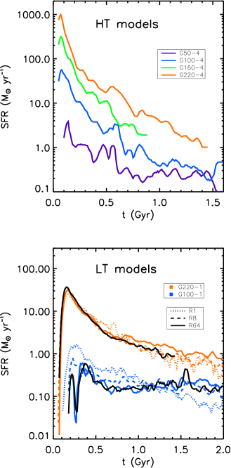
Figure 1.— (a) Time evolution of the SFRs in selected high-$T$ models as given in the legend. (b) Resolution study of low-$T$ models G100-1 (blue) and G220-1 (orange) with resolutions of R1 (dotted lines), R8 (dashed lines) and R64 (solid colored lines), where the resolution levels are in units of $10^{5}$ total particles. The standard R10 models (black) are shown for comparison.

The star formation rates in Figure 1 decline over time. Many of the models have SFR $>10\rm M_{\odot}$ yr^-1, corresponding to starburst galaxies. Some small or gas poor models such as G100-1, on the other hand, have SFR $<1\rm M_{\odot}$ yr^-1. They maintain slow but steady star formation over a long time and may represent quiescent normal galaxies. The maximum SFR appears to depend quantitatively on the initial instability of the disk as measured either by $Q_{sg,{\rm min}}$, the minimum Toomre parameter for the combination of stars and gas in the disk, or by the value for the gas only $Q_{g,{\rm min}}$. Figure 2 shows both correlations: $\log{\rm SFR}_{\rm max}\simeq 3.32-3.13Q_{sg,{\rm min}}$ and $\log{\rm SFR}_{\rm max}\simeq 2.76-1.99Q_{g,{\rm min}}$.

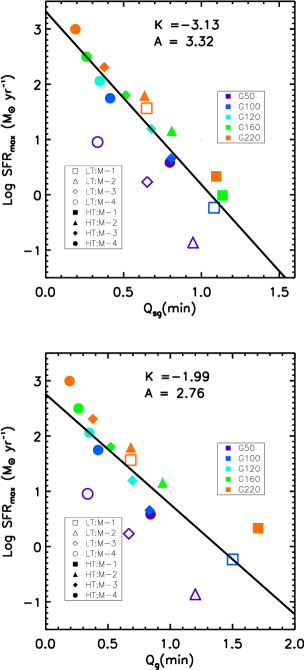
Figure 2.— Correlation between the maximum of the SFR and the minimum radial values of the Toomre instability parameters (a) for stars and gas together $Q_{sg,{\rm min}}$ and (b) for gas alone $Q_{g,{\rm min}}$. The solid lines are the least absolute deviation fits $\log{\rm SFR}_{\rm max}=K+AQ_{\rm min}$.

The SFRs in most models shown in Figure 1 appear to decline exponentially. From Paper I, the accumulated mass of the stars formed in each galaxy can be fitted with an exponential function:

$$\frac{M_{*}}{M_{\rm init}}=M_{0}\ \left[1-\exp\left({-t}/{\tau_{\rm SF}}\right)\right]\,,$$ (3)

where

$$M_{0}=0.96\ \epsilon_{\ell}\ \{1-2.9\ \exp\left[{-1.7}/{Q_{sg,{\rm min}}}\right]\}\,,$$ (4)

$$\tau_{\rm SF}=\left(34\pm 7\ \mbox{Myr}\right)\ \exp\left[Q_{sg,{\rm min}}/0.24\right],$$ (5)

$M_{\rm init}$ is the initial total gas mass, and $\tau_{\rm SF}$ is the star formation timescale. The star formation rate can then be rewritten in the following form:

$$\mbox{SFR}=\frac{dM_{*}}{dt}\propto\frac{1}{\tau_{\rm SF}}{\exp\left({-t}/{\tau_{\rm SF}}\right)}\,.$$ (6)

A similar exponential form is also reported by MacArthur et al. (2004), as first suggested by Larson (1974) and Tinsley & Larson (1978).

Sandage (1986) studied the star formation rate of different types of galaxies in the Local Group and proposed an alternative form for the star formation history, as explicitly formulated by MacArthur et al. (2004):

$$\mbox{SFR}\propto\frac{t}{\tau_{\rm SF}^{2}}\exp\left({-t^{2}}/{\tau_{\rm SF}^{2}}\right)$$ (7)

Figure 3a shows an example of model G220-1 (low-$T$) fitted with these two formula. Both formulae appear quite similar at intermediate times. The Sandage model captures the initial rise in star formation better, but the exponential form follows the late time behavior of our models more closely. As we only include stellar feedback implicitly by maintaining constant gas sound speed, we must be somewhat cautious about our interpretation of the late time results. In order to compare the fits, we define a parameter for relative goodness of the fit

$$\chi^{2}=\sum\left([y_{s}-y_{f}]/y_{m}\right)^{2}$$ (8)

where $y_{s}$ is the SFR from the simulation, $y_{m}$ is the maximum of SFR, and $y_{f}$ is the model function from equation (6) or (7). Note that since we do not take into account the uncertainty of each point, the absolute value of $\chi^{2}$ has no meaning. We only compare the relative $\chi^{2}$ values in Figure 3b. Both formulae fit equally well to many models, especially to those with high gas fractions that form a lot of stars early on. But for some models such as G100-1 (low-$T$) and G220-1 (high-$T$), the exponential function seems to fit noticeably better. Therefore we use the exponential form in the rest of the paper.

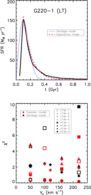
Figure 3.— (a) Example fit of the SFR evolution curve with the exponential form (eq. 6) and the Sandage (1986) form (eq. 7) for model G220-1 (low-$T$) as an example. (b) The relative goodness of fit $\chi^{2}$ (eq. 8) for all models for exponential (red) and Sandage (1986) (black) forms.

This analysis implies that the star formation history depends quantitatively on the initial gravitational instability of a galaxy after its formation or any major perturbation. An unstable galaxy forms stars rapidly in an early time, so its stellar populations will appear older than those in a more stable galaxy. More massive galaxies are less stable than small galaxies with the same gas fraction. The different star formation histories in such galaxies may account for the downsizing effect that star formation first occurs in big galaxies at high redshift, while modern starburst galaxies are smaller (Cowie et al. 1996; Poggianti et al. 2004; Ferreras et al. 2004), and thus more stable.

3.2. Radial Distribution of Gas and Star Formation

Figure 4 shows the radial distribution of different gas components and the SFR of selected models. The gas distribution and SFR are calculated at the star formation timescale $\tau_{\rm SF}$ derived from the fits given in Paper I. We assume that 70% of the gravitationally collapsed, high-density gas (as identified by sink particles) is in molecular form. Similarly, we identify unaccreted gas as being in atomic form. The total amount of gas is the sum of both components.

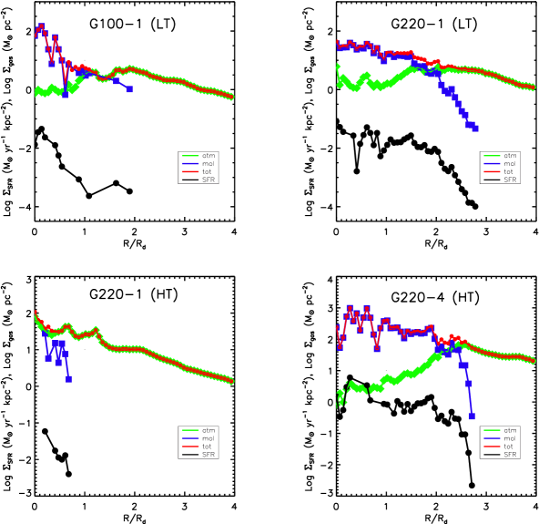
Figure 4.— Radial profiles of atomic (SPH particles; green dimond), molecular (70% of sink particle mass; blue square), and total (red dot) gas surface density, as well as SFR surface density (black dot). $R_{\rm d}$ is the radial disk scale length as given in Table 1. Note the solid lines are used to connect the symbols.

Figure 4 shows that the simulated disks have gas distributions that are mostly atomic in the outer disk but dominated by molecular gas in the central region. Observations by Wong & Blitz (2002) and Heyer et al. (2004) show that the density difference between the atomic and molecular components in the central region depends on the size and gas fraction of the galaxy. For example, $\Sigma_{\rm H_{2}}$ in the center of NGC4321 is almost two orders of magnitude higher than $\Sigma_{\rm H_{I}}$ (Wong & Blitz, 2002), while in M33, the difference is only about one order of magnitude (Heyer et al., 2004). A similar relation between the fraction of molecular gas and the gravitational instability of the galaxy is seen in our simulations. In our most unstable galaxies such as G220-4, the central molecular gas surface density exceeds the atomic gas surface density by more than two orders of magnitude, while in a more stable model like G220-1 (high $T$), the profiles of $\Sigma_{\rm H_{2}}$ and $\Sigma_{\rm H_{I}}$ are close to each other within one disk scale length $R_{\rm d}$.

We also find a linear correlation between the molecular gas surface density and the SFR surface density, as can be seen by their parallel radial profiles in Figure 4. (In operational terms, we find a correlation between the surface density in sink particles and the rate at which they accrete mass.) Gao & Solomon (2004b) found a tight linear correlation between the far infrared luminosity, a tracer of the star formation rate, and HCN luminosity, in agreement with our result that star formation rate and molecular gas have similar surface density profiles.

The agreement between the simulations and observations supports our assumption that both molecular gas and stars form by the gravitational collapse of high density gas. Note, however, that we neglect recycling of gas from molecular clouds back into the warm atomic and dissociated or ionized medium represented by SPH particles in our simulation. Although it is possible that even that reionized gas may still quickly collapse again if the entire region is gravitationally unstable, this still constitutes an important limitation of our models that will have to be addressed in future work.

4. GLOBAL SCHMIDT LAW

To derive the global Schmidt law from our models, we average $\Sigma_{\rm SFR}$ and $\Sigma_{\rm gas}$ over the entire star forming region of each galaxy. We define the star forming region following Kennicutt (1989), using a radius chosen to encircle 80% of the mass accumulated in sink particles (denoted $R_{80}$ hereafter). The SFR is taken from the SFR evolution curves at some chosen time. As mentioned in § 3, 30% of the mass of sink particles is assumed to be stars, while the remaining 70% of the sink particle mass remains in molecular form. The atomic gas component is computed from the SPH particles not participating in localized gravitational collapse, that is, gas particles not accreted onto sink particles. The total is the sum of atomic and molecular gas.

Figure 5 shows the global Schmidt laws derived from our simulations at the star formation time $t=\tau_{\rm SF}$ as listed in Table 1. Note that for a few models this is just the maximum simulated time, as indicated in Table 1. (Results from different times and star formation regions are shown in the next section.) We fit the data to the total gas surface density of the models listed in Table 1 (both low $T$ and high $T$). A least-square fit to the models we have run gives a simulated global Schmidt law

$$\Sigma_{\rm{SFR}}=(1.1\pm 0.4\times 10^{-4}\mbox{ M}_{\odot}\mbox{ yr}^{-1}\mbox{ kpc}^{-2})$$

$$\times\left(\frac{\Sigma_{\rm{gas}}}{1\ \rm M_{\odot}\ {\rm pc}^{-2}}\right)^{1.56\pm 0.09}$$ (9)

For comparison, the best fit to the observations by Kennicutt (1998b) gives a global Schmidt law for the total gas surface density in a sample that includes both the normal and starburst galaxies of

$$\Sigma_{\rm{SFR}}=(2.5\pm 0.7\times 10^{-4}\mbox{ M}_{\odot}\mbox{ yr}^{-1}\mbox{ kpc}^{-2})$$

$$\times\left(\frac{\Sigma_{\rm{gas}}}{1\ \rm M_{\odot}\ {\rm pc}^{-2}}\right)^{1.4\pm 0.15}.$$ (10)

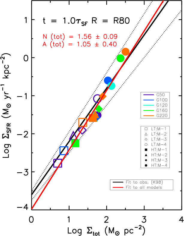
Figure 5.— A comparison of the global Schmidt laws between our simulations and the observations. The red line is the least-square fit to the total gas of the simulated models, the black solid line is the best fit of observations from Kennicutt (1998b), while the black dotted lines indicate the observational uncertainty. The color of the symbol indicates the rotational velocity for each model (see Table 1); labels from M-1 to M-4 are sub-models with increasing gas fraction; and open and filled symbols represent low and high $T$ models, respectively.

The global Schmidt law derived from the simulations agrees with the observed slope within the observational errors, but has a normalization a bit lower than the observed range. There are three potential explanations for this discrepancy. First, we have not weighted the fit by the actual distribution of galaxies in mass and gas fraction. Second, as we discuss in the next subsection, we have not used models at different times in their lives weighted by the distribution of lifetimes currently observed. Third, we have only simulated isolated, normal galaxies. Our models therefore do not populate the highest $\Sigma_{\rm SFR}$ values observed in Kennicutt (1998b), which are all starbursts occurring in interacting galaxies. These produce highly unstable disks that undergo vigorous starbursts with high SFR (e.g., Li, Mac Low & Klessen, 2004). Our result is supported by Boissier et al. (2003), who found a much deeper slope, $N\sim 2$ in a sample of normal galaxies comparable to our more stable models. In the models, the local SFE $\epsilon_{\ell}$ is fixed at 30%, independent of the galaxy model. A change of the assumed value of $\epsilon_{\ell}$ changes the normalization but not the slope of our relation. For example, an extremely high value of $\epsilon_{\ell}\sim 90$% increases $A$ to $\sim 3.15\times 10^{-4}\mbox{ M}_{\odot}\mbox{ yr}^{-1}\mbox{ kpc}^{-2}$, which is just within the $1\sigma$ upper limit of the observation by Kennicutt (1998b). If we decrease $\epsilon_{\ell}$ to 10%, then $A$ decreases to $\sim 0.7\times 10^{-4}\mbox{ M}_{\odot}\mbox{ yr}^{-1}\mbox{ kpc}^{-2}$. These fairly extreme assumptions still produce results lying within the observed ranges (e.g., Wong & Blitz, 2002), suggesting that our overall results are insensitive to the exact value of the local SFE that we assume.

The SFR surface densities $\Sigma_{\rm SFR}$ change dramatically with the gas fraction in the disk. The most gas-rich models (M-4, circles) have the highest $\Sigma_{\rm SFR}$, while the models poorer in gas (M-1, squares) have $\Sigma_{\rm SFR}$ two orders of magnitudes lower than their gas-rich counterparts. Note that models with lower $\Sigma_{\rm SFR}$ tend to have slightly higher scatter, because in these models fewer sink particles form, and they form over a longer period of time, resulting in higher statistical fluctuations.

A resolution study is shown in Figure 6 that compares the global Schmidt law computed with different numerical resolutions. Runs with different resolution converge within 10% in both the $\Sigma_{\rm SFR}$ and $\Sigma_{\rm gas}$. Although numerical resolution affects the total mass collapsed, and the number and location of fragments, as shown in Paper I, the SFR at $\tau_{\rm SF}$ seems to be less sensitive to the numerical resolution.

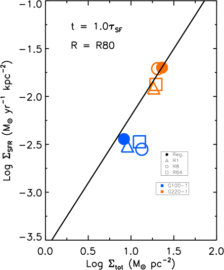
Figure 6.— Same as Figure 5 but for the resolution study of low $T$ models of G100-1 (blue) and G220-1 (orange). Models with total particle number of $N_{\rm tot}=10^{5}$ (R1; open triangle), $8\times 10^{5}$ (R8; open circle) and $6.4\times 10^{6}$ (R64; open square) are shown. Models with regular resolution $N_{\rm tot}=10^{6}$ (R10 filled circle) are also shown for comparison.

4.1. A Parameter Study

In order to test how sensitive the global Schmidt law is to the radius $R$ and the time $t$ chosen to measure it, we carry out a parameter study changing both $R$ and $t$ individually. To maintain consistency with the previous section, we continue to assume a constant local SFE $\epsilon_{\ell}=30$%. Figure 7 compares the global Schmidt laws in total gas at different radii for the star-forming region $R=R_{50}$ and $R_{100}$ (encircling 50% and 100% of the newly formed star clusters), while the time is fixed to $t=\tau_{\rm SF}$. We can see that the case with $R_{50}$ has larger scatter than that with $R_{100}$. This is due to the larger statistical fluctuations caused by the smaller number of star clusters within this radius. The global Schmidt law with $R=R_{100}$ is almost identical to that with $R=R_{80}$ shown in Figure 5.

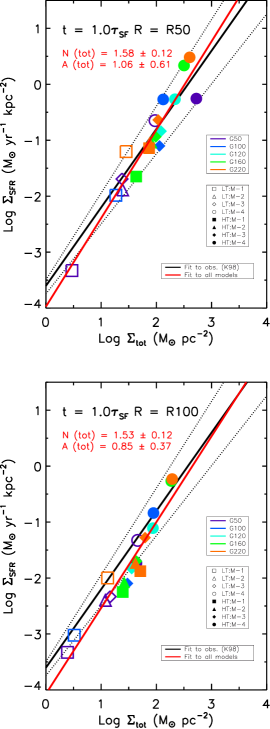
Figure 7.— Same as Figure 5 but with different radii assumed for the star-forming region: (a) $R=R_{50}$, and (b) $R=R_{100}$. The time is fixed at $t=\tau_{\rm SF}$.

Figure 8 compares the global Schmidt laws in total gas at different times $t=0.5\tau_{\rm SF}$ and $t=1.5\tau_{\rm SF}$ with the star formation radius fixed to $R_{80}$. Compared to the $t=\tau_{\rm SF}$ case, models in the $t=0.5\tau_{\rm SF}$ case have higher $\Sigma_{\rm SFR}$, because the SFR drops almost exponentially with time (§ 3.1). Similarly, models in the $t=1.5\tau_{\rm SF}$ case shift to the lower right. Nevertheless, data derived from different times appear to preserve the power-law index of the Schmidt law, just differing in the normalizations.

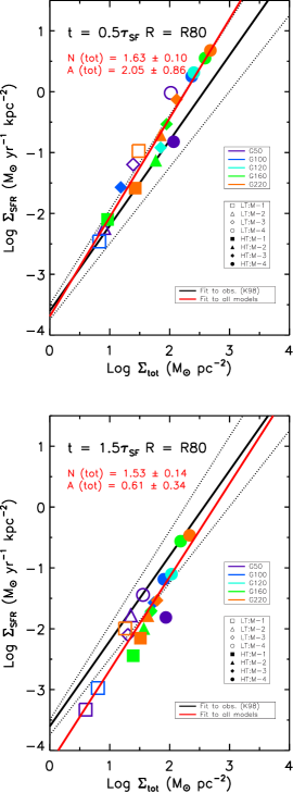
Figure 8.— Same as Figure 5 but derived at different times (a) $t=0.5\ \tau_{\rm SF}$ and (b) $t=1.5\ \tau_{\rm SF}$. The radius for the star formation region is fixed at $R_{80}$.

The global Schmidt law presented by Li et al. (2005b) was derived at a time when the total mass of the star clusters reached 70% of the maximum collapsed mass, which is close to 1.0 $\tau_{\rm SF}$ in many models. The time interval $\Delta t$ used to calculate the SFR was the time taken to grow from 30% to 70% of the maximum collapsed mass, rather than the $\Delta t=50$ Myr used here. Nevertheless, the results presented here also agree well with those in Li et al. (2005b).

Our parameter study demonstrates that the global Schmidt law depends only weakly on the details of how it is measured. The small scatter seen in Kennicutt (1998b) does suggest that additional physics not included in our modeling may be important. We should keep in mind that since we do not treat gas recycling, our models are valid only within one gas consumption time $\tau_{\rm SF}$. The evolution after that may become unrealistic as most of the gas is locked up in the sinks. Nevertheless, our results suggest that the Schmidt law is a universal description of gravitational collapse in galactic disks.

4.2. Alternative Global Star Formation Laws

The existence of a well-defined global Schmidt law suggests that the star formation rate depends primarily on the gas surface density. As shown by several authors (e.g., Quirk 1972; Larson 1988; Kennicutt 1989; Elmegreen 1994; Kennicutt 1998b), a simple picture of gravitational collapse on a free-fall timescale $\tau_{\rm ff}\propto\rho^{-1/2}$ qualitatively produces the Schmidt law. Assuming the gas surface density is directly proportional to the midplane density, $\Sigma_{\rm gas}\propto\rho$, it follows that $\Sigma_{\rm SFR}\propto\Sigma_{\rm gas}/\tau_{\rm ff}\propto\Sigma_{\rm gas}^{3/2}$. This suggests that the Schmidt law reflects the global growth rate of gas density under gravitational perturbations.

An alternative scenario that uses the local dynamical timescale has been suggested by several groups (e.g. Wyse 1986; Wyse & Silk 1987; Silk 1997; Elmegreen 1997; Hunter et al. 1998; Tan 2000). In particular, Elmegreen (1997) and Hunter et al. (1998) proposed a kinematic law that accounts for the stabilizing effect of rotational shear, in which the global SFR scales with the angular velocity of the disk,

$$\Sigma_{\rm SFR}\propto\frac{\Sigma_{\rm gas}}{t_{\rm orb}}\propto\Sigma_{\rm gas}\Omega$$ (11)

where $t_{\rm orb}$ is the local orbital timescale and $\Omega$ is the orbital frequency. Kennicutt (1998b) gave a simple form for the kinematical law,

$$\Sigma_{\rm SFR}\simeq 0.017\ \Sigma_{\rm gas}\Omega$$ (12)

with the normalization corresponding to a SFR of 21% of the gas mass per orbit at the outer edge of the disk.

For our analysis, we follow Kennicutt (1998b) and define $t_{\rm orb}=2\pi R/V(R)=2\pi/\Omega(R)$, where $V(R)$ is the rotational velocity at radius $R$. We use the initial rotational velocity, which should not change much with time as it depends largely on the potential of the dark matter halo. Figure 9 shows the relationship between $\Sigma_{\rm SFR}$ and $\Sigma_{\rm gas}\Omega$ in our models. The densities of SFR $\Sigma_{\rm SFR}$ and total gas $\Sigma_{\rm gas}$ are calculated the same way as in Figure 5 at 1.0 $\tau_{\rm SF}$ and $R_{80}$, and $\Omega(R)$ is calculated by using the initial total rotational velocity at $R_{80}$. A least-square fit to the data gives $\Sigma_{\rm SFR}=(0.036\pm 0.004)\times\left(\Sigma_{\rm gas}\Omega\right)^{1.49\pm 0.1}$. This correlation has a steeper slope than the linear law given in equation (12), suggesting a discrepancy between the behavior of our models and the observed kinematical law.

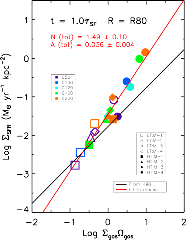
Figure 9.— Relation between $\Sigma_{\rm SFR}$ and $\Sigma_{\rm gas}\Omega$. The legends are the same as in Figure 5. The black solid line is the linear relationg derived from the observations by Kennicutt (1998b), as given in our equation (12).

However, Boissier et al. (2003) recently reported a slope of $\sim$ 1.5 for the kinematical law from observations of 16 normal disk galaxies, in agreement with our results. Examination of Figure 7 in Kennicutt (1998b) also shows that the normal galaxies, considered alone, seem to have a steeper slope than the galactic nuclei and starburst galaxies. Boissier et al. (2003) suggested several reasons for the discrepancy, the most important one being the difference between their sample of normal galaxies and the sample of Kennicutt (1998b) including many starburst galaxies and galaxy nuclei. More simulations, and models with higher SFR such as galaxy mergers are necessary to test this hypothesis.

4.3. A New Parameterization

The global Schmidt law describes global collapse in the gas disk. It does not seem to depend on the local star formation process. From Paper I and Li et al. (2005b) we know that $\Sigma_{\rm SFR}$ correlates tightly with the strength of gravitational instability (see also Mac Low & Klessen 2004; Klessen et al. 2000; Heitsch et al. 2001). Here we quantify this correlation, using the Toomre Q parameter to measure the strength of instability.

Figure 10 shows the correlation between $\Sigma_{\rm SFR}$ and the local gravitational instability parameters $Q_{\rm min}$. The parameters $Q_{\rm min}$ are minimum values of the Toomre $Q$ parameters for gas $Q_{g,{\rm min}}(t)$, and the combination of stars and gas $Q_{sg,{\rm min}}(t)$ at a given time $t$, respectively. To obtain the $Q$ parameters, we follow the approach of Rafikov (2001), as described in equations (1)–(3) of Paper I. We divide the entire galaxy disk at time $t$ into 40 annuli, calculate the $Q$ parameters in each annulus, then take the minimum. In the plots, the time when $\Sigma_{\rm SFR}$ is computed is $t=\tau_{\rm SF}$. This correlation does not change significantly with time, but the scatter becomes larger at later times because the disk becomes more clumpy, which makes the calculation of $Q_{g,{\rm min}}(t)$ more difficult (see below).

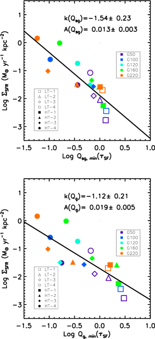
Figure 10.— Correlations between $\Sigma_{\rm SFR}$ and the minimum value of (a) the Toomre parameter for stars and gas $Q_{sg}(t)$ and (b) the Toomre parameter for gas $Q_{g}(t)$ at $t=1\ \tau_{\rm SF}$. The legends are the same as in Figure 5. The solid black lines are the least-square fits to the data given in equation (4.3).

There is substantial scatter in the plots, at least partly caused by the clumpy distribution of the gas. Equations (1)–(3) for the $Q$ parameters in Paper I are derived for uniformly distributed gas, such as in our initial conditions. As the galaxies evolve, the gas forms filaments or spiral arms probably leading to the fluctuations seen. The least-square fits to the data shown in Figure 10 give

$$\Sigma_{\rm SFR}=\left(0.013\pm 0.003\ \mbox{ M}_{\odot}\mbox{ yr}^{-1}\mbox{ kpc}^{-2}\right)$$

$$\times\left[Q_{sg,{\rm min}}(\tau_{\rm SF})\right]^{-1.54\pm 0.23}$$ (13)

$$\Sigma_{\rm SFR}=\left(0.019\pm 0.005\ \mbox{ M}_{\odot}\mbox{ yr}^{-1}\mbox{ kpc}^{-2}\right)$$

$$\times\left[Q_{g,{\rm min}}(\tau_{\rm SF})\right]^{-1.12\pm 0.21}$$ (14)

If we take a first-order approximation, $Q_{sg}\propto 1\ /\Sigma_{\rm gas}$, then equation (4.3) gives $\Sigma_{\rm SFR}\propto\Sigma_{\rm gas}^{1.54}$ at $t=\tau_{\rm SF}$, agreeing very well with the observations. The slopes derived from $Q_{g}$ appear to be lower than those derived from $Q_{sg}$, but are still within the slope range observed.

Keep in mind that the local instability is a non-linear interaction between the stars and gas, and so is much more complicated than the linear stability analysis presented here. Also, the instability of the entire disk at a certain time is not fully represented by the minimum values of the Q parameters we employ here, although they do represent the region of fastest star formation. These factors limit our ability to derive the global Schmidt law directly from the instability analysis.

5. LOCAL SCHMIDT LAW

The relationship between surface density of SFR $\Sigma_{\rm SFR}$ and gas density $\Sigma_{\rm gas}$ can also be measured as a function of radius within a galaxy, giving a local Schmidt law. Observations by Wong & Blitz (2002) and Heyer et al. (2004) show significant variations in both the indices $N$ and normalizations $A$ of the local Schmidt laws of individual galaxies. For example, Heyer et al. (2004) show that M33 follows the law

$$\Sigma_{\rm{SFR}}=(0.0035\pm 0.066\ \mbox{ M}_{\odot}\mbox{ yr}^{-1}\mbox{ kpc}^{-2})$$

$$\times\left({\Sigma_{\rm{tot}}}/{1\ \rm M_{\odot}\ {\rm pc}^{-2}}\right)^{3.3\pm 0.07},$$ (15)

while Wong & Blitz (2002) show that $N$ has a range of 1.23–2.06 in their sample.

To derive local Schmidt laws, we again divide each individual galaxy into 40 radial annuli within 4 $R_{\rm d}$, then compute $\Sigma_{\rm gas}$ and $\Sigma_{\rm SFR}$ in each annulus. The SFR is measured at $t=\tau_{\rm SF}$ as in § 4. For models where $\tau_{\rm SF}>3$ Gyr or is beyond the simulation duration, the maximum simulated timestep is used instead, as listed in Table 1.

5.1. Star Formation Thresholds

Figure 11 shows the relation between $\Sigma_{\rm SFR}$ and $\Sigma_{\rm gas}$ correlations for all models in the simulations that form stars in the first 3 Gyr. With such a large number of models in one plot, it is straightforward to characterize the general features, and to compare with the observations shown in Figure 3 of Kennicutt (1998b). Similar to the individual galaxies in Kennicutt (1998b) and Martin & Kennicutt (2001), each model here shows a tight $\Sigma_{\rm SFR}$–$\Sigma_{\rm gas}$ correlation, the local Schmidt law. However, $\Sigma_{\rm SFR}$ drops dramatically at some gas surface density. This is a clear indication of a star-formation threshold.

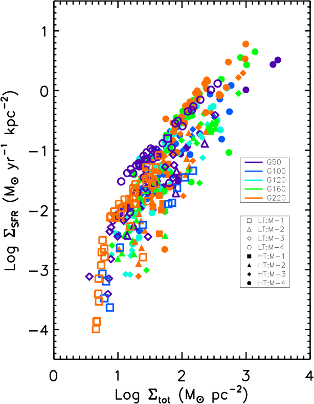
Figure 11.— Local Schmidt laws of all models with $\tau_{\rm SF}<3$ Gyr. The legends are the same as in Figure 5: the color of the symbol indicates the rotational velocity for each model as given in Table 1, the shape indicates the sub-model classified by gas fraction, and open and filled symbols represent low and high $T$ models, respectively.

We therefore define a threshold radius $R_{\rm th}$ as the radius that encircles 95% of the newly formed stars. The gas surface density at the threshold radius $R_{\rm th}$ in Figure 11 has a range from $\sim 4\rm{M}_{\odot}\ {pc}^{-2}$ for the relatively stable model G220-1 (low-$T$) to $\sim 60\rm{M}_{\odot}\ {pc}^{-2}$ for the most unstable model G220-4 (high-$T$). Note that in some galaxies, there are also smaller dips in SFR at higher density. Martin & Kennicutt (2001) suggest that rotational shearing can cause an inner star-formation threshold. However, the inner dips in our simulations are likely due to the lack of accretion onto sink particles in the simulations after most of the gas in the central region has been consumed. Further central star formation in real galaxies would occur due to gas recycling, which we neglect, and, probably more important, after interactions with other galaxies.

In the analysis of observations, a dimensionless parameter, $\alpha_{Q}=\Sigma_{\rm th}/\Sigma_{\rm crit}=1/Q$ has been introduced to relate the star formation threshold to the Toomre unstable radius (Kennicutt, 1989). The critical radius is usually defined as the radius where $Q_{g}=1$. With a sample of 15 spiral galaxies, Kennicutt (1989) found $\alpha_{Q}\simeq 0.63$ by assuming a constant effective sound speed (the velocity dispersion) of the gas $c_{s}=6$ km s^-1. This result was confirmed by Martin & Kennicutt (2001) with a larger sample of 32 well-studied nearby spiral galaxies, who reported a range of $\alpha_{Q}\sim 0.3$–1.2, with a median value of 0.69. However, Hunter et al. (1998) found $\alpha_{Q}\simeq 0.25$ for a sample of irregular galaxies with $c_{s}=9$ km s^-1. As pointed out by Schaye (2004), this derivation of $\alpha_{Q}$ depends on the assumption of $c_{s}$. The values of $\alpha_{Q}$ derived from our models using their actual values of $c_{s}$ as shown in Figure 12. We find that the value of $\alpha_{Q}$ depends not only on the gas sound speed, but also on the gas fraction of the galaxy. For models with the same rotational velocity and gas fraction, lower gas sound speed results in a higher value of $\alpha_{Q}$. For models with the same total mass and sound speed, higher gas fraction leads to higher $\alpha_{Q}$. The gas-poor models in our simulations ($f_{\rm g}=20\%$) have a range of $\alpha_{Q}\sim$ 0.2–1.0, agreeing roughly with observations. This again may reflect the relative stability of the nearby galaxies in the observed samples.

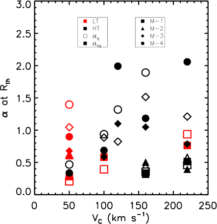
Figure 12.— The dimensionless parameter giving ratio of star formation threshold surface density to critical surface density for Toomre instability $\alpha_{Q}=1/Q_{\rm th}$ is shown for low-$T$ (in red) and high-$T$ (in black) models. Open symbols give values derived using gas only, $\alpha_{g}=1/Q_{g,{\rm th}}$, while filled symbols give values derived using both stars and gas, $\alpha_{sg}=1/Q_{sg,{\rm th}}$. Gas fraction of disks increases from M-1 to M-4 (see Table 1).

There are several theoretical approaches to explain the presence of star formation thresholds. Martin & Kennicutt (2001) suggest that the gravitational instability model explains the thresholds well, with the deviation of $\alpha_{Q}$ from one simply due to the non-uniform distribution of gas in real disk galaxies. Hunter et al. (1998) proposed a shear criterion for star forming dwarf irregular galaxies, as they appear to be sub-critical to the Toomre criterion. Schaye (2004) modeled the thermal and ionization structure of a gaseous disk. He found the critical density is about $\Sigma_{\rm crit}\sim 3$–10 $\rm{M}_{\odot}\ \rm{pc}^{-2}$ with a gas velocity dispersion of $\sim$ 10 km s^-1, and argued that thermal instability determines the star formation threshold in the outer disk. Our models suggest that the threshold depends on the gravitational instability of the disk. The derived $\Sigma_{\rm crit}$ and $\alpha_{Q}$ from our stable models ($Q_{sg,{\rm min}}>1$) agree well with observations, supporting the arguments of Martin & Kennicutt (2001).

5.2. Local Correlations Between Gas and Star Formation Rate

We fit the local Schmidt law to the total gas surface density within $R_{\rm th}$, as demonstrated in Figure 13. The models in Figure 13 all have the same rotational velocity of 220 km s^-1 but different gas fractions and sound speeds. The local Schmidt laws of these models vary only slightly in slope and normalization.

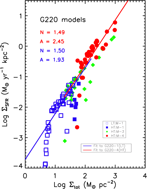
Figure 13.— Comparisons of local Schmidt laws of galaxy models with the same rotational velocity of 220 km s^-1 but different gas fractions and sound speeds, as indicated in the legend. The solid lines are least-square fits to data points within the threshold radius $R_{\rm th}$.

Figures 14a and 14b compare the slope $N$ and normalization $A$ of the local Schmidt laws for all models in Table 1 that form stars in the first 3 Gyr. The slope of the fit to the total gas in Figure 14a varies from about 1.2 to 1.7. Larger galaxies tend to have larger $N$. However, the average slope is around 1.3, agreeing reasonably well with that of the global Schmidt law.

There is substantial fluctuation in the normalization of fits to the total gas, as shown in Figure 14(b). The variation is more than an order of magnitude, with gas-rich models tending to have high $A$. However, the average value of $A$ settles around 2.2, agreeing surprisingly well with that of the global Schmidt law. Overall, the averaged local Schmidt law gives:

$$\Sigma_{\rm{SFR}}=(2.46\pm 1.62\times 10^{-4}\ \mbox{ M}_{\odot}\ \mbox{ yr}^{-1}\mbox{ kpc}^{-2})$$

$$\times\left(\frac{\Sigma_{\rm{tot}}}{1\ \rm M_{\odot}\ {\rm pc}^{-2}}\right)^{1.31\pm 0.15}$$ (16)

Figure 14.— Local Schmidt law (a) slope $N$ and (b) normalization $A$ for all models with $\tau_{\rm SF}<3$ Gyr. The fit is to the total gas surface density $\Sigma_{\rm tot}$ within the threshold radius $R_{\rm th}$. The symbols represent different models, as indicated in the legends. The dotted line in each panel indicates the linearly averaged value across the models shown.

The averaged local Schmidt law is very close to the global Schmidt law in § 4.

The average slope in equation (5.2) is rather smaller than the value of $N=3.3$ observed by Heyer et al. (2004) in M33. The galaxy M33 is very interesting. It is a nearly isolated, small disk galaxy with low luminosity and low mass. It has total mass of $M_{\rm tot}\sim 10^{11}\ \rm M_{\odot}$ and a gas mass of $\rm M_{\rm gas}\sim 8.0\times 10^{9}\ \rm M_{\odot}$ (Heyer et al., 2004). It is molecule-poor and sub-critical, with gas surface density is much smaller than the threshold surface density for star formation found by Martin & Kennicutt (2001). However, it is actively forming stars (Heyer et al., 2004). We do not have a model that exactly resembles M33, although a close one might be model G100-1 in terms of mass. However, the gas velocity dispersion of M33 is unknown, so we cannot make a direct comparison with our G100-1 models. In Figure 14, the low-$T$ model G100-1 has $N\sim 1.4$, but we have not derived a value for its high-$T$ counterpart, as it does not form stars at all in the first 3 Gyrs. Any stars that form in a disk similar to this will likely form in spiral arms or other nonlinear density perturbations that are not well characterized by an azimuthally averaged stability analysis. If these perturbations occur in the highest surface density regions as might be expected, the local Schmidt law will have a very high slope as observed. This speculation will need to be confirmed with models reaching higher mass resolution in the future. The details of the feedback model and equation of state may also begin to play a role in this extreme case.

The averaged values of our derived local Schmidt laws do agree well with the observations by Wong & Blitz (2002) of a number of other nearby galaxies. The similarity between the global and local Schmidt laws suggests a common origin of the correlation between $\Sigma_{\rm{SFR}}$ and $\Sigma_{\rm{gas}}$ in gravitational instability.

6. STAR FORMATION EFFICIENCY

The SFE is poorly understood, because it is difficult in both observations and simulations to determine the timescale for gas removal and the gaseous and stellar mass within the star formation region. On the molecular cloud scale, observations of several nearby embedded clusters with mass $M<1000\rm M_{\odot}$ indicate that the SFEs range from approximately 10–30% (Lada & Lada, 2003). However, it is thought that field stars form with SFE of only 1–5% in giant molecular clouds (e.g., Duerr, Imhoff, & Lada 1982), while the formation of a bound stellar cluster requires a local SFE $\gtrsim$ 20–50% (e.g., Wilking & Lada 1983; Elmegreen & Efremov 1997). An analytical model including outflows by Matzner & McKee (2000) suggests that the efficiency of cluster formation is in the range of 30–50%, and that of single star formation could be anywhere in the range 25–70%.

In the analysis of our simulations presented here, we convert the mass of the sink particles into stars using a fixed local SFE $\epsilon_{\ell}=30$%, consistent with both the observations and theoretical predictions mentioned above. This local efficiency is different from the global star formation efficiency in galaxies $\epsilon_{g}\leq\epsilon_{\ell}$, which measures the fraction of the total gas turned into stars. On a galactic scale, the star formation efficiency appears to be associated with the fraction of molecular gas (e.g., Rownd & Young 1999). The global SFE has had values derived from observations over a wide range, depending on the gas distribution and the molecular gas fraction (Kennicutt, 1998b). For example, in normal galaxies $\epsilon_{g}\simeq 2$–10%, while in starburst galaxies $\epsilon_{g}=10$–50%, with a median value of 30%. One factor that appears to contribute to the differences in $\epsilon_{g}$ is the gas content. The global SFE is generally averaged over all gas components, but since star formation correlates tightly with the local gravitational instability one expects higher global SFE in more unstable galaxies. In fact, as pointed out by Wong & Blitz (2002), most normal galaxies in the sample of Kennicutt (1998b) are molecule-poor galaxies, which seem to have high stability and low SFE, while molecule-rich starburst galaxies appear to be unstable, forming stars with high efficiency.

The variation of the normalization of the local Schmidt laws in § 5 also suggests that the global SFE varies from galaxy to galaxy. To quantitatively measure the SFE in our models, we apply the common definition of the global SFE,

$$\epsilon_{g}=M_{*}/(M_{*}+M_{\rm gas})=M_{*}/M_{\rm init}$$ (17)

over a period of $10^{8}$ years, an average timescale for star formation in galaxy. In this equation, $M_{*}=\epsilon_{\ell}M_{\rm sink}$ is the mass of newly formed stars, and $M_{\rm gas}$ includes both the remaining mass of the sink particles and the SPH particles, so that $M_{*}+M_{\rm gas}=M_{\rm init}$ is the total mass of the initial gas.

Figure 15(a) and (b) show the relation between the minimum values of the initial $Q$ parameter $Q_{sg,{\rm min}}$ and the global SFE normalized by the local SFE $\epsilon_{\rm g}/\epsilon_{\ell}$. The time period is taken as the first 100 Myr after star formation starts. If we take $\epsilon_{\ell}$ as a constant for all models, it appears that $\epsilon_{g}$ declines as $Q_{sg,{\rm min}}$ increases. Therefore, $\epsilon_{g}$ is high in less stable galaxies with high mass or high gas fraction. A least-absolute-deviation fit of the data gives a linear fit of $\epsilon_{g}/\epsilon_{\ell}=0.9-0.97\ Q_{sg,{\rm min}}$. This fit is good for values of $Q_{sg,{\rm min}}\leq 1$. For more stable galaxies, with larger values of $Q_{sg,{\rm min}}$, the SFE remains finite, deviating from the linear fit.

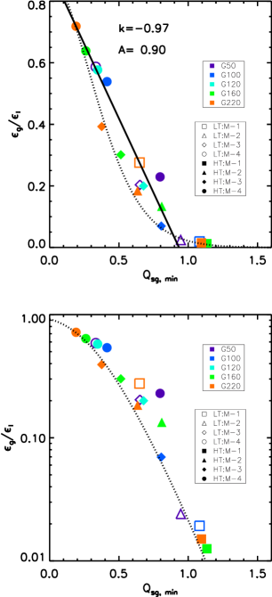
Figure 15.— The global SFE normalized by the local one $\epsilon_{\rm g}/\epsilon_{\ell}$ versus the minimum initial gravitational instability parameter $Q_{sg,{\rm min}}$ in linear (a) and log space (b). The legends are the same as in Figure 5. The black solid line is the least-absolute-deviation fit to the data, while the dotted line is the function given in equation (6).

Using the empirical relations we have derived from our models earlier in the paper, we can derive a better analytic expression for $\epsilon_{g}$. Equation (17) can be combined with equation (3) in § 3.1 to yield an equation for the global SFE

$$\epsilon_{g}=M_{0}\left[1-\exp\left({-t}/{\tau_{\rm SF}}\right)\right]$$ (18)

We evaluate this at $t=100$ Myr, taking the definitions of $M_{0}$ and $\tau_{\rm SF}$ derived from equations (4) and (5). Normalizing by the local SFE, we find

$$\epsilon_{g}/\epsilon_{\ell}=0.96\times\left[1-2.88\exp\left({-1.7}/{Q_{sg,{\rm min}}}\right)\right]$$

$$\times\left[1-\exp\left(-2.9e^{-Q_{sg,{\rm min}}/0.24}\right)\right]$$ (19)

The function given by equation (6) is shown in Figure 15. For $Q_{sg,{\rm min}}\leq 1.0$ it is well approximated by the much simpler linear function

$$\epsilon_{g}/\epsilon_{\ell}\simeq 0.9-Q_{sg,{\rm min}}$$ (20)

as shown in Figure 15(a). At larger values of $Q_{sg,{\rm min}}$, the exact function predicts the SFE in our models excellently as shown in Figure 15(b). Observational verification of this behavior is vital.

7. ASSUMPTIONS AND LIMITATIONS OF THE MODELS

7.1. Isothermal Equation of State

One of the two central assumptions in our model is the use of an isothermal equation of state to represent a constant velocity dispersion. This is of course a simplification, as the interstellar medium in reality has a broad range of temperatures 10 K$<T<10^{7}$ K. However, neutral gas velocity dispersions in normal spiral galaxies cover a far more limited range, as reviewed by Kennicutt (1998b); Elmegreen & Scalo (2004); Scalo & Elmegreen (2004) and Dib et al. (2005). The characteristic $\sigma$ increases when the averaged $\Sigma_{\rm SFR}$ of a galaxy reaches tens of solar masses per year, but the normal galaxies in the sample with reliable measurements lie in the range $\sim$7–13 km s^-1 (e.g., Elmegreen & Elmegreen 1984; Meurer et al. 1996; van Zee et al. 1997; Stil & Israel 2002; Hippelein et al. 2003).

At least two mechanisms appear viable for maintaining roughly constant velocity dispersion for the bulk of the gas in a galactic disk, supernova feedback and magnetorotational instability (Mac Low & Klessen, 2004). Three-dimensional simulations in a periodic box with parameters characteristic of the outer parts of galactic disks by Dib et al. (2005) show that supernova driving leads to constant velocity dispersions of $\sigma\sim$ 6 km s^-1 for the total gas and $\sigma_{\rm H_{\rm I}}\sim$ 3 km s^-1 for the H_I gas, independent of the supernova rate. Simulations of the feedback effects across whole galactic disks do suggest that the inner parts have slightly higher velocity dispersions (e.g. Thacker & Couchman 2000), though within the range that we consider. The magnetorotational instability in galactic disks was suggested by Sellwood & Balbus (1999) to maintain the observed velocity dispersion, a suggestion that has since been substantiated by both local (Piontek & Ostriker, 2005) and global (Dziourkevitch, Elstner, & Rüdiger, 2004) numerical models. This may act even in regions with little or no active star formation.

Recently, Robertson et al. (2004) presented simulations of galactic disks and claimed that an isothermal equation of state leads to a collapsed disk as the gas fragments into clumps that fall to the galactic center due to dynamical friction. However, similar behavior is seen in models by Immeli et al. (2004) who did not use an isothermal equation of state, but also ran at resolutions not satisfying the Jeans criterion (Bate & Burkert, 1997; Truelove et al., 1997). On the other hand, using essentially the same code and galaxy model as Robertson et al. (2004), but with higher resolution satisfying the Jeans criterion, we do not see this collapse. Insufficient resolution that fails to resolve the Jeans mass leads to spurious, artificial fragmentation and thus collapse.

Simulations by Governato et al. (2004) suggest that some long-standing problems in galaxy formation such as the compact disk and lack of angular momentum may well be due to insufficient resolution or violation of numerical criteria. Our results lead us to agree that the isothermal equation of state is not the cause of the compact disk problem, but rather inadequate numerical resolution.

Our assumption of an isothermal equation of state does, of course, rule out the treatment by our model of phenomena such as galactic winds associated with the hot phase of the interstellar medium (although the venting of supernova energy vertically may help maintain the isothermal behavior of the gas in the plane). The strong starbursts produced in some of our galaxy models will certainly cause strong galactic winds. It remains unclear whether even strong starbursts can remove substantial amounts of gas, though. Certainly they cannot in small galaxies (Mac Low & Ferrara, 1999), and larger galaxies would seem more resistant to stripping in starbursts than smaller ones. However, galactic winds will certainly influence the surroundings of starburst galaxies, as well as their observable properties. These effects should eventually be addressed in future simulations with more comprehensive gas physics and a more realistic description of the feedback from star formation.

7.2. Sink Particles

The use of sink particles enables us to directly identify high gas density regions, measure gravitational collapse, and follow the dynamical evolution of the system to a long time. We can therefore determine the star formation morphologies and rates, and study the Schmidt laws and star formation thresholds.

However, one shortcoming of our sink particle implementation is that we do not include gas recycling. Once the gas collapses into the sinks, it remains locked up there. As discussed in Paper I, the bulk of the gas that does not form stars will remain in the disk and contribute to the next cycle of star formation. Also, the ejected material from massive stars will return into the gas reservoir for future star formation. Another problem is accretion. In the current model, sink particles accrete until the surrounding gas is completely consumed. However, in real star clusters, the accretion would be cut-off due to stellar radiation, and the clusters will actually lose mass due to outflow and tidal stripping.

These shortcomings of our sink particle technique may contribute to two limitations of our models: first, the decline of star formation rate over time due to consumption of the gas, as seen in Figure 1; second, the variation of SFR over time in the simulated global Schmidt laws in Figure 8. Nevertheless, as we have demonstrated in the previous sections, our models are valid within one gas consumption time $\tau_{\rm SF}$, and are sufficient to investigate the dominant physics that controls gravitational collapse and star formation within that period.

7.3. Initial Conditions of Galaxies

Many nearby galaxies appear to be gas-poor and stable ($Q_{sg}>1$). However, their progenitors at high redshift were gas rich, so the bulk of star formation should have taken place early on. In order to test this, we vary the gas fraction (in terms of total disk mass) in the models. We also vary the total galaxy mass and thus the rotational velocity. These result in different initial stability curves. Massive, or gas-rich galaxies have low values of the $Q$ parameters, so they are unstable, forming stars quickly and efficiently.

There are no observations yet that directly measure the $Q$ values in starburst galaxies. However, indirectly, observations by Dalcanton et al. (2004) show that dust lanes, which trace star formation, only form in unstable regions. Moreover, observations of color gradients in disk galaxies by MacArthur et al. (2004) show that massive galaxies form stars earlier and with higher efficiency. Both of these observations are naturally explained by our models.

The Toomre $Q$ parameter for gas $Q_{g}$ differs from that for a combination of stars and gas $Q_{sg}$ in some of our model galaxies. This leads to slightly different results in Figure 3 and Figure 10 where we compare $Q_{sg,{\rm min}}$ and $Q_{g,{\rm min}}$. However, we believe $Q_{sg}$ is a better measure of gravitational instability in the disk, as it takes into account both the collisionless and the collisional components, and the interaction between them. We note that it is a simplified approach to quantify the instability of the entire disk with just a number $Q_{sg,{\rm min}}$, as $Q$ has a radial distribution, evolves with time, and is an azimuthally averaged quantity, but nevertheless, we find interesting regularities by making this approximation.

8. SUMMARY

We have simulated gravitational instability in galaxies with sufficient resolution to resolve collapse to molecular cloud pressures in models of a wide range of disk galaxies with different total mass, gas fraction, and initial gravitational instability. Our calculations are based on two approximations: the gas of the galactic disk has an isothermal equation of state, representing a roughly constant gas velocity dispersion; and sink particles are used to follow gravitationally collapsed gas, which we assume to form both stars and molecular gas. With these approximations, we have derived star formation histories; radial profiles of the surface density of molecular and atomic gas and SFR; both the global and local Schmidt laws for star formation in galaxies; and the star formation efficiency.

The star formation histories of our models show the exponential dependence on time given by equation 6 in agreement with, for example, the interpretation of galactic color gradients by MacArthur et al. (2004). The radial profiles of atomic and molecular gas qualitatively agree with those observed in nearby galaxies, with surface density of molecular gas peaking centrally at values much above that of the atomic gas (e.g. Wong & Blitz, 2002). The radial profile of the surface density of SFR correlates linearly with that of the molecular gas, agreeing with the observations of Gao & Solomon (2004b).

Our models quantitatively reproduce the observed global Schmidt law (Kennicutt, 1998b)—the correlation between the surface density of star formation rate $\Sigma_{\rm{SFR}}$ and the gas surface density $\Sigma_{\rm{gas}}$—in both the slope and normalization over a wide range of gas surface densities (eq. 4). We show that $\Sigma_{\rm SFR}$ is strongly correlated with the gravitational instability of galaxies $\Sigma_{\rm SFR}\propto\left[Q_{sg,{\rm min}}(\tau_{\rm SF})\right]^{-1.54\pm 0.23}$, where $Q_{sg,{\rm min}}(\tau_{\rm SF})$ is the local instability parameter at time $t=\tau_{\rm SF}$ (see eq. 4.3). This correlation naturally leads to the Schmidt law.

On the other hand, our models do not reproduce the correlation $\Sigma_{\rm SFR}\sim\Sigma_{\rm gas}\Omega$ derived from kinematical models (Kennicutt, 1998b). However, they may agree better with the dependence of the normal galaxies on this quantity, as suggested by Boissier et al. (2003). The discrepancy may be caused by the lack of extreme starburst galaxies such as galaxy mergers in our set of models.

The local Schmidt laws of individual galaxies clearly show evidence of star formation thresholds above a critical surface density. The threshold surface density varies with galaxy, and appears to be determined by the gravitational stability of the disk. The derived threshold parameters for our stable models cover the range of values seen in observations of normal galaxies. The local Schmidt laws have significant variations in both slope and normalization, but also cover the observational ranges reported by Wong & Blitz (2002), Boissier et al. (2003) and Heyer et al. (2004). The average normalization and slope of the local power-laws are very close to those of the global Schmidt law.

Our models show that the global star formation efficiency (SFE) $\epsilon_{g}$ can be quantitatively predicted by the gravitational instability of the disk. We have used a fixed local SFE $\epsilon_{\ell}=30\%$ to convert the mass of the sink particles to stars in our analysis. This is a reasonable assumption for the SFE in dense, high pressure molecular clouds. The global SFE of a galaxy then can be shown to depend quantitatively on a nonlinear function (eq. 6) of the minimum Toomre parameter $Q_{sg,{\rm min}}$ for stars and gas that can be approximated for $Q_{sg,{\rm min}}\leq 1.0$ with the linear correlation $\epsilon_{\rm g}/\epsilon_{\ell}\propto 0.9-Q_{sg,{\rm min}}$. More unstable galaxies have higher SFE. Massive, or gas-rich galaxies in our suite of models are unstable, forming stars quickly with high efficiency. They represent starburst galaxies. Small, or gas-poor galaxies are rather stable, forming stars slowly with low efficiency, corresponding to quiescent, normal galaxies.

Table 1Galaxy Models and Numerical Parameters

Model	$f_{\rm g}$	$R_{\rm d}$	$Q_{sg}$(LT)	$Q_{sg}$(HT)	$N_{\rm tot}$	$h_{\rm g}$	$m_{\rm g}$	$\tau_{\rm SF}$(LT)	$\tau_{\rm SF}$(HT)
G50-1	0.2	1.41	1.22	1.45	1.0	10	0.08	4.59	$\cdots$
G50-2	0.5	1.41	0.94	1.53	1.0	10	0.21	1.28	$\cdots$
G50-3	0.9	1.41	0.65	1.52	1.0	10	0.37	0.45	$\cdots$
G50-4	0.9	1.07	0.33	0.82	1.0	10	0.75	0.15	0.53
G100-1	0.2	2.81	1.08	1.27	6.4	7	0.10	2.66	$\cdots$
G100-2	0.5	2.81	$\cdots$	1.07	1.0	10	1.65	$\cdots$	$\cdots$
G100-3	0.9	2.81	$\cdots$	0.82	1.0	10	2.97	$\cdots$	1.92
G100-4	0.9	2.14	$\cdots$	0.42	1.0	20	5.94	$\cdots$	0.15
G120-3	0.9	3.38	$\cdots$	0.68	1.0	20	5.17	$\cdots$	0.46
G120-4	0.9	2.57	$\cdots$	0.35	1.0	30	10.3	$\cdots$	0.16
G160-1	0.2	4.51	$\cdots$	1.34	1.0	20	2.72	$\cdots$	3.1
G160-2	0.5	4.51	$\cdots$	0.89	1.0	20	6.80	$\cdots$	0.58
G160-3	0.9	4.51	$\cdots$	0.52	1.0	30	12.2	$\cdots$	0.30
G160-4	0.9	3.42	$\cdots$	0.26	1.5	40	16.3	$\cdots$	0.11
G220-1	0.2	6.20	0.65	1.11	6.4	15	1.11	0.28	3.0
G220-2	0.5	6.20	$\cdots$	0.66	1.2	30	14.8	$\cdots$	0.39
G220-3	0.9	6.20	$\cdots$	0.38	2.0	40	15.9	$\cdots$	0.25
G220-4	0.9	4.71	$\cdots$	0.19	4.0	40	16.0	$\cdots$	0.096

References

- Barnes (2002) Barnes, J. E. 2002, MNRAS, 333, 481
- Barnes & Hernquist (1996) Barnes, J. E., & Hernquist, L. 1996, ApJ, 471, 115
- Bate et al. (1995) Bate, M. R., Bonnell, I. A., & Price, N. M. 1995, MNRAS, 277, 362
- Bate & Burkert (1997) Bate, M. R., & Burkert, A. 1997, MNRAS, 288, 1060
- Ballesteros-Paredes et al. (1999) Ballesteros-Paredes, J., Hartmann, L., & Vázquez-Semadeni, E. 1999, ApJ, 527, 285
- Ballesteros-Paredes & Mac Low (2002) Ballesteros-Paredes, J., & Mac Low, M.-M. 2002, ApJ, 570, 734
- Bell & de Jong (2000) Bell, E. F., & de Jong, R. S. 2000, MNRAS, 312, 497
- Bergin et al. (2004) Bergin, E. A., Hartmann, L. W., Raymond, J. C., & Ballesteros-Paredes, J. 2004, ApJ, 612, 921
- Boissier et al. (2003) Boissier, S., Prantzos, N., Boselli, A., & Gavazzi, G., 2003, MNRAS, 346, 1215
- Cowie et al. (1996) Cowie, L. L., Songaila, A., Hu, E. M., & Cohen, J. G. 1996, AJ, 112, 839
- Dalcanton et al. (2004) Dalcanton, J. J., Yoachim, P., & Bernstein, R. A. 2004, ApJ, 608, 189
- Dib et al. (2005) Dib, S., Bell, E., & Burkert, A. 2005, astro-ph/0506339
- Dickey, Hanson, & Helou (1990) Dickey, J. M., Hanson, M. M., & Helou, G. 1990, ApJ, 352, 522
- Duerr, Imhoff, & Lada (1982) Duerr, R., Imhoff, C. L., & Lada, C. J. 1982, ApJ, 261, 135
- Dziourkevitch, Elstner, & Rüdiger (2004) Dziourkevitch, N., Elstner, D., & Rüdiger, G. 2004, A&A, 423, L29
- Elmegreen (1994) Elmegreen, B. G. 1994, ApJ, 425, 73
- Elmegreen (1997) Elmegreen, B. G. 1997, Rev. Mex. Astron. Astrofis. Ser. Conf., 6, 165
- Elmegreen & Efremov (1997) Elmegreen, B. G. & Efremov, Y. N. 1997, ApJ, 480, 235
- Elmegreen (2002) Elmegreen, B. G. 2002, ApJ, 577, 206
- Elmegreen & Elmegreen (1984) Elmegreen, D. M., & Elmegreen, B. G. 1984, ApJS, 54, 127
- Elmegreen & Parravano (1994) Elmegreen, B. G., & Parravano, A., 1994, ApJ, 435, 121
- Elmegreen & Scalo (2004) Elmegreen, B. G., & Scalo, J. 2004, ARA&A, 42, 275
- Ferguson et al. (1998) Ferguson, A. M. N., Wyse, R. F. G., Gallagher, J. S., & Hunter, D. A. 1998, ApJ, 506, 19
- Ferreras et al. (2004) Ferreras, I., Silk, J., Böhm, A., & Ziegler, B. 2004, MNRAS, 355, 64
- Friedli & Benz (1993) Friedli, D., & Benz, W. 1993, A&A, 268, 65
- Friedli & Benz (1995) Friedli, D., & Benz, W. 1995, A&A, 301, 649
- Friedli et al. (1994) Friedli, D., Benz, W., & Kennicutt, R. 1994, ApJ, 430, L105
- Gao & Solomon (2004a) Gao, Y., & Solomon, P. M. 2004a, ApJS, 152, 63
- Gao & Solomon (2004b) Gao, Y., & Solomon, P. M. 2004b, ApJ, 606, 271
- Gerritsen & Icke (1997) Gerritsen, J. P. E. & Icke, V. 1997, å, 325, 972
- Glover & Mac Low (2005) Glover, S., & Mac Low, M.-M. 2005, in preparation
- Governato et al. (2004) Governato, F., Mayer, L., Wadsley, J., Gardner, J. P., Willman, B., Hayashi, E., Quinn, T., Stadel, J., & Lake, G. 2004, ApJ, 607, 688
- Hartmann (2000) Hartmann, L. 2000, in 33d ESALAB Symp., Star Formation from the Small to the Large Scale, ed. F. Favata, A. Kaas, & A. Wilson (ESA SP-445; Noordwijk: ESA), 107
- Hartmann et al. (2001) Hartmann, L., Ballesteros-Paredes, J., & Bergin, E. A. 2001, ApJ, 562, 852
- Heitsch et al. (2001) Heitsch, F., Mac Low, M.-M., & Klessen, R. S., 2001, ApJ, 547, 280
- Heyer et al. (2004) Heyer, M. H., Corbelli, E., Schneider, S. E., & Young, J. S. 2004, ApJ, 602, 723
- Hippelein et al. (2003) Hippelein, H., Haas, M., Tuffs, R. J., Lemke, D., Stickel, M., Klaas, U., & Völk, K. J. 2003, 407, 137
- Hollenbach, Werner, & Salpeter (1971) Hollenbach, D. J., Werner, M. W., & Salpeter, E. E. 1971, ApJ, 163, 165
- Hunter et al. (1998) Hunter, D. A., Elmegreen, B. G., & Baker, A. L. 1998, ApJ, 493, 595
- Immeli et al. (2004) Immeli, A., Samland, M., Gerhard, O., & Westera, P. 2004 A&A, 413, 547
- Jappsen et al. (2005) Jappsen, A., Klessen, R. S., Larson, R. B., Li, Y., & Mac Low, M.-M. 2005, A&A, 435, 611
- Katz (1992) Katz, N. 1992, ApJ, 391, 502
- Katz & Gunn (1991) Katz, N., & Gunn, J. E. 1991, ApJ, 377, 365
- Kamphuis & Sancisi (1993) Kamphuis, J., & Sancisi, R. 1993, A&A, 273, L31
- Kauffmann et al. (2003) Kauffmann, G. et al. 2003, MNRAS, 341, 54
- Kennicutt (1989) Kennicutt, R. C. 1989, ApJ, 344, 685
- Kennicutt (1998a) Kennicutt, R. C. 1998a, ARA&A, 36, 189
- Kennicutt (1998b) Kennicutt, R. C. 1998b, ApJ, 498, 541 (K98)
- Klessen (2000) Klessen, R. S. 2000, ApJ, 535, 869
- Klessen et al. (2000) Klessen, R. S., Heitsch, F., & Mac Low, M.-M. 2000, ApJ, 535, 887
- Klessen & Lin (2003) Klessen, R. S., & Lin, D. 2003, Phys. Rev. E, 046311, 1
- Kravtsov (2003) Kravtsov, A. V. 2003, ApJ, 590, L1
- Krumholz & McKee (2005) Krumholz, M. R., & McKee, C. F., 2005, ApJ, in press (astro-ph/0505177)
- Lada & Lada (2003) Lada, C. J., & Lada, E. A. 2003, ARA&A, 41, 57
- Larson (1974) Larson, R. B. 1974, MNRAS, 166, 585
- Larson (1988) Larson, R. B. 1988, in Galactic and Extragalactic star formation, ed. R.E. Pudritz & M. Fich (Dordrecht: Kluwer), 435
- Larson (2003) Larson, R. B. 2003, Rep. Prog. Phys., 66, 1651
- Li et al. (2003) Li, Y., Klessen, R. S., & Mac Low, M.-M. 2003, ApJ, 592, 975
- Li et al. (2004) Li, Y., Mac Low, M.-M., & Klessen, R. S. 2004, ApJ, 614, L29
- Li et al. (2005a) Li, Y., Mac Low, M.-M., & Klessen, R. S. 2005a, ApJ, 626, 823 (PaperI)
- Li et al. (2005b) Li, Y., Mac Low, M.-M., & Klessen, R. S. 2005b, ApJ, 620, L19
- MacArthur et al. (2004) MacArthur, L. A., Courteau, S., Bell, E., & Holtzman, J. 2004, ApJS, 152, 175
- Mac Low (1999) Mac Low, M.-M. 1999, ApJ, 524, 169
- Mac Low et al. (2005) Mac Low, M.-M., Balsara, D. S., Kim, J., & de Avillez, M. A. 2005, ApJ, 626, 864
- Mac Low & Klessen (2004) Mac Low, M.-M., & Klessen, R. S. 2004, Rev. Mod. Phys., 76, 125
- Mac Low & Ferrara (1999) Mac Low, M.-M., & Ferrara, A. 1999, ApJ, 513, 142
- Martin & Kennicutt (2001) Martin, C. L., & Kennicutt, R. C. 2001, ApJ, 555, 301
- Matzner & McKee (2000) Matzner, C. D., & McKee, C. F. 2000, ApJ, 545, 364
- Meurer et al. (1996) Meurer, G. R., Carignan, C., Beaulieu, S. F., & Freeman, K. C. 1996, AJ, 111, 1551
- Mihos & Hernquist (1994) Mihos, J. C., & Hernquist, L. 1994, ApJ, 427, 112
- Mo et al. (1998) Mo, H. J., Mao, S., & White, S. D. M. 1998, MNRAS, 295, 319
- Navarro & Benz (1991) Navarro, J. F., & Benz, W. 1991, ApJ, 380, 320
- Navarro et al. (1995) Navarro, J. F., Frenk, C. S., & White, S. D. M. 1995, MNRAS, 275, 56
- Navarro et al. (1997) Navarro, J. F., Frenk, C. S., & White, S. D. M. 1997, ApJ, 490, 493
- Noguchi (2001) Noguchi, M. 2001, ApJ, 555, 289
- Okamoto et al. (2005) Okamoto, T., Eke, V. R., Frenk, C. S., & Jenkins, A. 2005, MNRAS, in press
- Ostriker, Gammie, & Stone (1999) Ostriker, E. C., Gammie, C. F., & Stone, J. M. 1999, ApJ, 513, 259
- Padoan & Nordlund (2002) Padoan, P., & Nordlund, Å. 2002, ApJ, 576, 870
- Passot & Vázquez-Semadeni (1998) Passot, T., & Vázquez-Semadeni, E. 1998, Phys. Rev. E, 58, 450
- Piontek & Ostriker (2005) Piontek, R. A., & Ostriker, E. C. 2005, ApJ, 629, 849
- Poggianti et al. (2004) Poggianti, B. M., Bridges, T. J., Komiyama, Y., Yagi, M., Carter, D., Mobasher, B., Okamura, S., & Kashikawa, N. 2004, ApJ, 601, 197
- Quirk (1972) Quirk, W. J. 1972, ApJ, 176, L9
- Rafikov (2001) Rafikov, R. R. 2001, MNRAS, 323, 445
- Robertson et al. (2004) Robertson, B., Yoshida, N., Springel, V., & Hernquist, L. 2004, ApJ, 606, 32
- Rownd, Dickey, & Helou (1994) Rownd, B. K., Dickey, J. M., & Helou, G. 1994, ApJ, 108, 1683
- Rownd & Young (1999) Rownd, B. K., & Young, J. S. 1999, AJ, 118, 670
- Sandage (1986) Sandage, A. 1986, A&A, 161, 89
- Scalo et al. (1998) Scalo, J., Vázquez-Semadeni, E., Chappell, D., & Passot, T. 1998, ApJ, 504, 835
- Scalo & Elmegreen (2004) Scalo, J., & Elmegreen, B. G. 2004, ARA&A, 42, 275
- Schaye (2004) Schaye, J. 2004, ApJ, 609, 667
- Schmidt (1959) Schmidt, M. 1959, ApJ, 129, 243
- Searle, Sargent & Bagnuolo (1973) Searle, L., Sargent, W. L. W., & Bagnuolo, W. G. 1973, ApJ, 179, 427
- Sellwood & Balbus (1999) Sellwood, J. A., & Balbus, S. A. 1999, ApJ, 511, 660
- Shu et al. (1987) Shu, F. H., Adams, F. C., & Lizano, S. 1987, ARA&A, 25, 23
- Silk (1997) Silk, J. 1997, ApJ, 481, 702
- Sommer-Larsen & Dolgov (2001) Sommer-Larsen, J., & Dolgov, A. 2001, ApJ, 551, 608
- Sommer-Larsen et al. (2003) Sommer-Larsen, J., Götz, M., & Portinari, L. 2003, ApJ, 596, 47
- Sommer-Larsen et al. (1999) Sommer-Larsen, J., Gelato, S., & Vedel, H. 1999, ApJ, 519, 501
- Springel (2000) Springel, V. 2000, MNRAS, 312, 859
- Springel & Hernquist (2003) Springel, V., & Hernquist, L. 2003, MNRAS, 339, 289
- Springel et al. (2005) Springel, V., Di Matteo, T., & Hernquist, L. 2005, ApJ, 620, L79
- Springel & White (1999) Springel, V., & White, S. D. M. 1999, MNRAS, 307, 162
- Springel et al. (2001) Springel, V., Yoshida, N., & White, S. D. M. 2001, New Astron., 6, 79
- Steinmetz & Mueller (1994) Steinmetz, M., & Mueller, E. 1994, A&A, 281, L97
- Steinmetz & Navarro (1999) Steinmetz, M., & Navarro, J. F. 1999, ApJ, 513, 555
- Steinmetz & White (1997) Steinmetz, M., & White, S. D. M. 1997, MNRAS, 288, 545
- Stil & Israel (2002) Stil, J. M., & Israel, F. P. 2002, A&A, 392, 473
- Struck-Marcell (1991) Struck-Marcell, C. 1991, ApJ, 368, 348
- Struck & Smith (1999) Struck, C. & Smith, D. C. 1999, ApJ, 527, 673
- Tan (2000) Tan, J. C. 2000, ApJ, 536, 173
- Thacker & Couchman (2000) Thacker, R. J. & Couchman, H. M. P. 2000, ApJ, 545, 728
- Tinsley & Larson (1978) Tinsley, B. M. & Larson, R. B. 1978, ApJ, 221, 554
- Toomre (1964) Toomre, A. 1964, ApJ, 139, 1217
- Toomre (1977) Toomre, A. 1977, ARA&A, 15, 437
- Truelove et al. (1997) Truelove, J. K., Klein, R. I., McKee, C. F., Holliman, J. H., Howell, L. H., & Greenough, J. A. 1997, ApJ, 489, L179
- van den Hoek et al. (2000) van den Hoek, L. B., de Blok, W. J. G., van der Hulst, J. M., & de Jong, T. 2000, ApJ, 357, 397
- Vader & Vigroux (1991) Vader, J. P., & Vigroux, L. 1991, å, 246, 32
- van der Hulst et al. (1993) van der Hulst, J. M., Skillman, E. D., Smith, T. R., Bothun, G. D., McGaugh, S. S., & de Blok, W. J. G. 1993, AJ, 106, 548
- van der Kruit & Shostak (1982) van der Kruit, P. C., & Shostak, G. S. 1982, A&A, 105, 351
- van Zee et al. (1997) van Zee, L., Haynes, M., Salzer, J. J., & Broeils, A. H. 1997, AJ, 113, 5
- Vázquez-Semadeni et al. (2004) Vázquez-Semadeni, E., Kim, J., Shadmehri, M., & Ballesteros-Paredes, J. 2005, ApJ, 618, 344
- Wada & Norman (2001) Wada, K., & Norman, C. A. 2001, ApJ, 547, 172
- Walborn et al. (1999) Walborn, N. R., Barbá, R. H., Brandner, W., Rubio, M., Grebel, E. K., & Probst, R. G. 1999, AJ, 117, 225
- Whitworth (1998) Whitworth, A. P. 1998, MNRAS, 296, 442
- Wilking & Lada (1983) Wilking, B. A., & Lada, C. J. 1983, ApJ, 274, 698
- Wong & Blitz (2002) Wong, T., & Blitz, L. 2002, ApJ, 569, 157
- Wyse (1986) Wyse, R. 1986, ApJ, 311, L41
- Wyse & Silk (1987) Wyse, R., & Silk, J. 1987, ApJ, 339, 700
- Young et al. (1996) Young, J. S., Allen, L., Kenney, J. D. P., Lesser, A., & Rownd, B. 1996, AJ, 112, 1903