On the large-angle anomalies of the microwave sky

Abstract

We apply the multipole vector framework to full-sky maps derived from the first year WMAP data. We significantly extend our earlier work showing that the two lowest cosmologically interesting multipoles, $\ell=2$ and $3$, are not statistically isotropic. These results are compared to the findings obtained using related methods. In particular, we show that the planes of the quadrupole and the octopole are unexpectedly aligned. Moreover, the combined quadrupole plus octopole is surprisingly aligned with the geometry and direction of motion of the solar system: the plane they define is perpendicular to the ecliptic plane and to the plane defined by the dipole direction, and the ecliptic plane carefully separates stronger from weaker extrema, running within a couple of degrees of the null-contour between a maximum and a minimum over more than $120\degr$ of the sky. Even given the alignment of the quadrupole and octopole with each other, we find that their alignment with the ecliptic is unlikely at $>98$% C.L., and argue that it is in fact unlikely at $>99.9$% C.L. Most of the $\ell=2$ and $3$ multipole vectors of the known Galactic foregrounds are located far from those of the observed sky, strongly suggesting that residual contamination by such foregrounds is unlikely to be the cause of the observed correlations. Multipole vectors, like individual $a_{\ell m}$, are very sensitive to sky cuts, and we demonstrate that analyses using cut skies induce relatively large errors, thus weakening the observed correlations but preserving their consistency with the full-sky results. Similarly, the analysis of COBE cut-sky maps shows increased errors but is consistent with WMAP full-sky results. We briefly extend these explorations to higher multipoles, noting again anomalous deviations from statistical isotropy and comparing with ecliptic asymmetry manifest in the WMAP team’s own analysis. If the correlations we observe are indeed a signal of non-cosmic origin, then the lack of low-$\ell$ power will very likely be exacerbated, with important consequences for our understanding of cosmology on large scales.

1 Introduction

Following a series of increasingly successful experiments measuring the anisotropy of the cosmic microwave background (CMB), full-sky maps obtained by the Wilkinson Microwave Anisotropy Probe (WMAP) in its first year of observation have revolutionized the study of the CMB sky (Bennett et al., 2003a, b; Hinshaw et al., 2003a). In particular, a number of cosmological parameters have been determined with high accuracy (Spergel et al., 2003). Moreover, a WMAP-type survey opens a unique window to the physics of the early universe (Peiris et al., 2003) and enables tests of the standard inflationary picture, which predicts a CMB temperature anisotropy pattern that is nearly scale-free, statistically isotropic and, to the accuracy of all current or planned CMB experiments, Gaussian random (terms that we shall define more carefully below). Consequently, WMAP data led to many studies of Gaussianity (Komatsu et al., 2003; Park, 2004; Chiang et al., 2003; Magueijo & Medeiros, 2004; Vielva et al., 2004; Mukherjee & Wang, 2004; McEwen et al., 2005; Cruz et al., 2005; Eriksen et al., 2005; Larson & Wandelt, 2004; Naselsky et al., 2005a, b; Tojeiro et al., 2005; Cayon et al., 2005) and statistical isotropy (Eriksen et al., 2004b; Hajian & Souradeep, 2003; Hajian et al., 2005; Hajian & Souradeep, 2005; Hansen et al., 2004a, b; Prunet et al., 2005; Donoghue & Donoghue, 2005) of the CMB. While there was no significant evidence for the violation of Gaussianity and statistical isotropy in the pre-WMAP era, some of the aforementioned post-WMAP studies found evidence for violation of either Gaussianity or statistical isotropy, or both.

Arguably, the biggest surprises were to be found in temperature anisotropies on the largest angular scales. Most prominent among the “low-$\ell$ anomalies” is the near vanishing of the two-point angular correlation function $C(\theta)$ at angular separations greater than about 60 degrees (Spergel et al., 2003), confirming what was first measured using the Cosmic Background Explorer’s Differential Microwave Radiometer (COBE-DMR) a decade ago (Hinshaw et al., 1996). Beyond this long-standing anomaly in the overall amplitude of the large-angle fluctuations, it has also been noted that the octopole of the CMB is planar and oriented parallel to the quadrupole (Tegmark et al., 2003; de Oliveira-Costa et al., 2004). Furthermore, three of the four planes determined by the quadrupole and octopole are orthogonal to the ecliptic at a level inconsistent with Gaussian random, statistically isotropic skies at $99.8$% C.L., while the normals to these planes are aligned at $99.9$% C.L. with the direction of the cosmological dipole and with the equinoxes (Schwarz et al., 2004). These peculiar correlations presumably are connected to north-south asymmetry in the angular power spectrum (Eriksen et al., 2004b) and in the statistics of the extrema (Wandelt et al., 2004). Finally, there is a suggestion that the presence of preferred directions in the microwave background multipoles extends beyond the octopole to higher multipoles (Land & Magueijo, 2005a) and that there is an associated mirror symmetry (Land & Magueijo, 2005c).

The correct explanation of these unexpected correlations of the low-$\ell$ features of the microwave background with each other and with the solar system is currently not known. There are four possibilities: (1) there is a systematic error (an error in the data analysis or instrument characterization), (2) the source is astrophysical (i.e. an unexpected foreground), (3) it is cosmological in nature (e.g. an anisotropic universe, such as one with nontrivial topology), or (4) the observed correlations are a pure statistical fluke. The evidence for many of these low-$\ell$ correlations is strong ($>99$% C.L.) and presented with a variety of different methods (see, for example, Tegmark et al. (2003); Schwarz et al. (2004); Land & Magueijo (2005a); Hansen et al. (2004b); Eriksen et al. (2004b)). It is therefore unlikely that all of them are mere accidents. In this paper, we will at least attempt to clarify which of these and other correlations is likely to be a statistical fluke. Whatever the source of these correlations, until they are understood, cosmological inferences drawn from low-$\ell$ WMAP data (including polarization data), such as the possibility of early reionization, should be viewed with a healthy dose of skepticism.

This paper has two principal goals. First, we would like to further develop the theory of multipole vectors, a new representation of microwave background anisotropy introduced by Copi et al. (2004). In particular, we derive several new results, and comment on various ideas and results on the tests of Gaussianity and statistical isotropy that were subsequently presented by others using the multipole vectors or their variants. Our second major goal is to present a detailed analysis of the large-angle correlations discussed in Schwarz et al. (2004) and extend them in several directions.

The paper is organized as follows. In Sec. 2, we introduce the WMAP maps and their treatment used in our analysis. In Sec. 3, we review the theory behind the multipole vectors, derive several new results, and comment on other recent work on this topic. Section 4 deals in more detail with the morphology of the quadrupole and octopole. In Sec. 5, we introduce various statistics to quantify the low-$\ell$ correlations, extend our analysis to higher $\ell$, and present the results. Section 6 includes a detailed analysis of the issue of foregrounds and Sec. 7 describes the cut-sky reconstruction algorithm and results based on reconstructed maps. In Sec. 8, we present a comparison to COBE. The correlations of the WMAP angular power spectrum with the ecliptic plane is discussed in Sec. 9. We conclude in Sec. 10.

2 The microwave background sky

The temperature fluctuations of the microwave background $\Delta T(\theta,\phi;\mn@boldsymbol{x},t)$ are, in principle, functions of both the direction of observation $(\theta,\phi)$, and the location, $\mn@boldsymbol{x}$, and time, $t$, of the observation. In practice, essentially all our observations occur within the solar system and over a cosmologically short period of time, so we can ignore any local spatial and temporal variations in the microwave background. Our observations in each wavelength band are therefore the intensity of the microwave background radiation as a function of direction on the celestial sphere.

2.1 The standard representation

The most common representation of a real scalar function, $f(\theta,\phi)$, on the sphere is as an expansion in terms of multipole moments

$$f(\theta,\phi)=\sum_{\ell=0}^{\infty}f_{\ell}(\theta,\phi)$$ (1)

where the $\ell$-th multipole, $f_{\ell}(\theta,\phi)$, is typically given by

$$f_{\ell}(\theta,\phi)=\sum_{m=-\ell}^{\ell}a_{\ell m}Y_{\ell m}(\theta,\phi).$$ (2)

Here $Y_{\ell m}(\theta,\phi)$ are the standard spherical harmonic functions. For $f_{\ell}(\theta,\phi)$ real the complex coefficients $a_{\ell m}$ need to satisfy the reality condition $a_{\ell m}^{*}=(-1)^{m}a_{\ell,-m}$ and for fixed $\ell$ we have $2\ell+1$ independent, real degrees of freedom.

Standard cosmological theory predicts that the CMB fluctuations sample a statistically isotropic, Gaussian random field of zero mean. “Gaussian random” means that the real and imaginary parts of the $a_{\ell m}$ are each an independent random variable that is distributed according to a Gaussian distribution of zero mean. In principle, the variances of these Gaussian distributions (which, by the nature of a Gaussian, fully characterize the distribution) could be different for each $\ell$ and $m$ and for both the real and imaginary parts. “Statistically isotropic” means that, instead, these variances depend only on $\ell$. Thus, the expectation of any pair of $a_{\ell m}$ is

$$\left<a_{\ell^{\prime}m^{\prime}}^{*}a_{\ell m}\right>={\cal C}_{\ell}\delta_{\ell^{\prime}\ell}\delta_{m^{\prime}m},$$ (3)

where ${\cal C}_{\ell}$ is the expected power in the $\ell$th multipole and its (standard) observable estimator is

$$C_{\ell}\equiv\frac{1}{2\ell+1}\sum_{m=-\ell}^{\ell}\left|a_{\ell m}\right|^{2}.$$ (4)

The set of estimators $\{C_{\ell}\mid\ell=0,\ldots,\infty\}$ is called the angular power spectrum. The cosmic variance in the estimators is

$${\rm Var}(C_{\ell})=2{\cal C}_{\ell}^{2}/(2\ell+1).$$ (5)

Since the distributions of Gaussian variables are completely determined by their means and variances (and since the $a_{\ell m}$ have zero means), if the microwave background sky is indeed a realization of a Gaussian random, statistically isotropic process, then all of the accessible information in a microwave background temperature map about the underlying physics is contained in the angular power spectrum. (Non-linear growth of fluctuations will cause departures from Gaussianity. However, these departures are small at the large angular scales we will be considering.)

As mentioned in the introduction, many studies have been done looking for evidence of non-Gaussianity or deviations from statistical isotropy in the microwave background. A significant difficulty is that in the absence of particular models the range of possible manifestations of non-Gaussianity and statistical-anisotropy is enormous. Statistics that measure one manifestation well, can be entirely insensitive to another. Limits on particular statistics should be viewed in that light. Another conceptual and practical difficulty is separating tests of Gaussianity from tests of statistical isotropy. If statistical isotropy, $\left<a_{\ell^{\prime}m^{\prime}}^{*}a_{\ell m}\right>\propto\delta_{\ell^{\prime}\ell}\delta_{m^{\prime}m}$, is violated, then it is unclear how one can test Gaussianity, since each $a_{\ell m}$ could have its own independent distribution for which we are provided just one sample.

2.2 Full-sky maps

In this work, we use three full-sky maps based on the original single-frequency WMAP maps. The first two, the Internal Linear Combination (ILC) map and the Lagrange Internal Linear Combination (LILC) map, are minimum-variance maps obtained from WMAP’s single-frequency maps by Bennett et al. (2003a) (the WMAP team) and by Eriksen et al. (2004a), respectively. The third map is the cleaned full-sky map of Tegmark et al. (2003) (henceforth the TOH map). The full-sky maps may have residual foreground contamination that is mainly due to imperfect subtraction of the Galactic signal. Furthermore, the full-sky maps have complicated noise properties (Bennett et al., 2003a) that make them less than ideal for cosmological tests. While one can, in principle, straightforwardly compute the true (full-sky) multipole vectors from the single-frequency maps with the sky cut (as explicitly shown for an isolatitude sky cut in Sec. 7), a Galaxy cut larger than a few degrees will introduce a significant uncertainty in the reconstructed multipole vectors and consequently any statistics.

Nevertheless, there are compelling reasons why we believe the results of the analysis of the full-sky maps. First, all of the results are robust with respect to choice of the map, despite the fact that the ILC and LILC maps were obtained using a different method than the TOH map. This suggests that the full-sky maps indeed resemble the true Galaxy-subtracted microwave sky. Furthermore, one can show that the dominant component of the bias inherent in creating an ILC-type map has a quadrupolar pattern, and in particular looks like the spherical harmonic $Y_{20}$ with an amplitude of $\la 20\;\mathrm{\mu K}$ (H.K. Eriksen, private communication). For the quadrupole and octopole the dominant contributions to the Galactic foregrounds are a linear combination of $Y_{20}$ and ${\rm Re}(Y_{31})$, which is easily seen from the symmetry of the Galaxy (approximately north-south and east-west symmetric with a hot spot at the Galactic center and a cold spot at the anti-center). Indeed, the sum of the synchrotron, free-free and dust WMAP foreground maps (Bennett et al., 2003a) in the V-band gives $a_{20}=-217\;\mathrm{\mu K}$ and ${\rm Re}(a_{31})=88\;\mathrm{\mu K}$. These two modes make up about $90$% of the power in the quadrupole and octopole foregrounds. The next important modes in the WMAP foreground maps turn out to be $\mathrm{Re}(Y_{22})$ and $\mathrm{Re}(Y_{33})$. The quoted $20\;\mathrm{\mu K}$ uncertainty in the ILC-type map for the quadrupole can thus be understood as a $10$% uncertainty in the understanding of our galaxy. The uncertainty in the octopole is considerably smaller ($\la 10\;\mathrm{\mu K}$). As shown in Schwarz et al. (2004) and further demonstrated in Sec. 6, this Galactic contamination, even if present, would lead to Galactic and not the observed ecliptic (Solar System) correlations.

2.3 Methodological differences between the minimal variance maps

The guiding principle in the construction of the WMAP ILC, TOH and LILC full-sky maps is to search for a temperature map with minimal variance. For the convenience of the reader we summarize the essential steps that lead to the cleaned full-sky maps (see the original papers for full details).

In all three approaches, the input are the five WMAP frequency maps (K, Ka, Q, V and W band). The bands differ in a number of ways including noise properties and angular resolution. While the ILC and LILC map reduce all five bands to the K band resolution, the TOH map makes use of the higher resolution of the higher frequency bands. Each map can be written as

$$T(\nu_{i})=T_{\rm CMB}+T_{\rm residual}(\nu_{i}).$$ (6)

A combined map is created by the linear combination

$$T=T_{\rm CMB}+\sum_{i=1}^{5}w_{i}T_{\rm residual}(\nu_{i}),$$ (7)

with $\sum_{i}w_{i}=1$. Now it is assumed that the residuals (noise and foregrounds) and the CMB are uncorrelated, so that

$${\rm Var}(T)={\rm Var}(T_{\rm CMB})+{\rm Var}\left(\sum_{i=1}^{5}w_{i}T_{\rm residual}(\nu_{i})\right).$$ (8)

The idea is now to determine the 4 independent weights by minimizing the variance with respect to all pixels of a region of the sky. The ILC and LILC maps use the same 12 regions of the sky, whereas the TOH map uses 9 regions. For the ILC and LILC maps the weights are constants within a region of the sky, whereas for the TOH map the weights depend on multipole number $\ell$ (the minimization is done in spherical harmonic space instead of pixel space). The regions are selected according to the level of foreground contamination. To produce the final maps a Gaussian smoothing is applied to soften the edges. We see that the TOH map on the one hand and the ILC and LILC maps on the other hand use different procedures. The ILC and LILC maps differ mainly in the detailed implementation of the method. The drawback of the minimal variance method is that large CMB fluctuations tend to be canceled by large artificial foregrounds in order to obtain a small variance.

We shall see that, despite the differences between the three maps, the results of our analysis are very similar. This robustness argues strongly in favor of the legitimacy of using these full-sky maps for multipole vector analysis.

2.4 Kinetic quadrupole correction

By far the largest signal in the microwave background anisotropy is the dipole, recently measured by WMAP (Bennett et al., 2003b) to be $(3.346\pm 0.017)\;\mathrm{mK}$ in the direction $(l=263\aas@@fstack{\circ}85\pm 0\aas@@fstack{\circ}1,b=48\aas@@fstack{\circ}25\pm 0\aas@@fstack{\circ}04)$ in Galactic coordinates. This is nearly two orders of magnitude larger than the root-mean-square (rms) anisotropy in the dipole-subtracted sky, and so thought not to be of cosmological origin, but rather to be caused by the motion of the solar system with respect to the rest frame defined by the CMB. As shown by Peebles & Wilkinson (1968), the dipole induced by a velocity $v$ is $\bar{T}(v/c)\cos\theta$, where $\theta$ is measured from the direction of motion. Given $\bar{T}=(2.725\pm 0.002)\;\mathrm{K}$ (Mather et al., 1999), one infers that $v\simeq 370\;\mathrm{km\,s^{-1}}$.

The solar motion also implies the presence of a kinematically induced Doppler quadrupole (DQ; Peebles & Wilkinson 1968; Kamionkowski & Knox 2003). To second order in $\beta\equiv v/c\simeq 10^{-3}$, the specific intensity of the CMB for an observer moving with respect to the CMB rest-frame includes the usual monopole term with a black-body spectrum ($\propto x^{3}/[e^{x}-1]$, where $x=h\nu/[k_{\rm B}T]$); a dipolar term $\propto\cos\theta$, linear in $\beta$, with a dipole spectrum ($\propto x^{4}e^{x}/[e^{x}-1]^{2}$, the same as for primordial anisotropies); and a quadrupolar term $\propto 3\cos^{2}\theta-1$, quadratic in $\beta$, with a quadrupole spectrum ($\propto x^{5}e^{x}[e^{x}+1]/[e^{x}-1]^{3}$). Higher multipoles are induced only at higher order in $\beta$ and so can be neglected.

To first approximation the quadrupole spectrum differs very little from the dipole spectrum across the frequency range probed by WMAP. The DQ is itself a small contribution to the quadrupole. It has a total band-power of only $3.6\;\mathrm{\mu K}^{2}$ compared to $123.4\;\mathrm{\mu K}^{2}$ from the cut-sky WMAP analysis (Hinshaw et al., 2003a), $195.1\;\mathrm{\mu K}^{2}$ extracted (de Oliveira-Costa et al., 2004) from the ILC map (Bennett et al., 2003b), $201.6\;\mathrm{\mu K}^{2}$ from the TOH map (Tegmark et al. (2003)) or $350.6\;\mathrm{\mu K}^{2}$ from the LILC map (Eriksen et al. (2004a)). Therefore, it is a good approximation to treat the Doppler-quadrupole as having a dipole spectrum plus a small spectral distortion which we shall ignore. We can then readily subtract the DQ from any microwave background map.

The kinetic quadrupole is a very small contribution to the total theoretical power in the quadrupole, however, it gives rise to non-negligible contributions to some of the $a_{2m}$. This is due partially to the low power in the observed quadrupole and partially to the “orthogonality” of the correction (the correction is $m$ dependent and the largest corrections are not to the largest $a_{2m}$). This is a well known, well understood physical correction to the quadrupole that is often ignored. This correction must be applied when studying the alignment of the quadrupole, leaving it out introduces a correctable systematic error. Though it has little effect on the power in the quadrupole, it has a noticeable effect on the quadrupole orientation as shown below. We again stress that it is the orientation of the correction that makes it important. A quadrupole correction of this size pointing in a random direction would typically not lead to noticeable alignment changes.

Figures 1, 2, and 3 show the Doppler corrected quadrupole, the octopole, and their sum, for the TOH map in Galactic coordinates in Mollweide projection. The corresponding multipoles from the ILC and LILC maps are very similar.

3 Multipole vectors

Multipole vectors provide an alternative representation of the complete set of information represented by the full-sky map. They represent a radical reorganization of the information that nevertheless retains the integrity of the individual multipoles. Moreover, the information is arranged in such away as to be independent of the choice of coordinate system. Therefore the multipole vectors may be a superior representation for probing the null hypothesis of statistical isotropy, and for looking for signatures of specific effects that might pick out special directions on the sky due to nonstandard inflationary physics, systematic artifacts in the map-making, unexpected foregrounds, cosmic topology, deviations from General Relativity, or other unknown effects.

3.1 Definition

In the multipole vector representation, $f_{\ell}(\theta,\phi)$ is written in terms of a scalar, $A^{(\ell)}$ and $\ell$ unit vectors, $\left\{\hat{\mn@boldsymbol{v}}^{(\ell,j)}\mid j=1,\ldots,\ell\right\}$:

$$f_{\ell}(\theta,\phi)=A^{(\ell)}\left[\prod_{i=1}^{\ell}\left(\hat{\mn@boldsymbol{v}}^{(\ell,i)}\cdot{\hat{\mn@boldsymbol{e}}}\right)-{\cal T}_{\ell}\right].$$ (9)

Here $\hat{\mn@boldsymbol{e}}$ is the (radial) unit vector in the $(\theta,\phi)$ direction. (Henceforth, we will use $\hat{\mn@boldsymbol{e}}$ and $(\theta,\phi)$ interchangeably.) In Cartesian coordinates, $\hat{\mn@boldsymbol{e}}=(\sin\theta\cos\phi,\sin\theta\sin\phi,\cos\theta)$. $\mathcal{T}_{\ell}$ is the sum of all possible traces of the first term; rendering the full expression traceless. In this context, a trace means replacing a product of dipoles $\left(\hat{\mn@boldsymbol{v}}^{(\ell,i)}\cdot{\hat{\mn@boldsymbol{e}}}\right)\left(\hat{\mn@boldsymbol{v}}^{(\ell,j)}\cdot{\hat{\mn@boldsymbol{e}}}\right)$, by $\left(\hat{\mn@boldsymbol{v}}^{(\ell,i)}\cdot\hat{\mn@boldsymbol{v}}^{(\ell,j)}\right)$. Equation (9) can also be written as

$$f_{\ell}(\hat{\mn@boldsymbol{e}})=A^{(\ell)}\left[\hat{\mn@boldsymbol{v}}^{(\ell,1)}\cdots\hat{\mn@boldsymbol{v}}^{(\ell,\ell)}\right]_{TF}^{i_{1}\cdots i_{\ell}}\left[{\hat{\mn@boldsymbol{e}}}\cdots{\hat{\mn@boldsymbol{e}}}\right]^{TF}_{i_{1}\cdots i_{\ell}}$$ (10)

where $\left[\cdots\right]_{TF}$ denote the trace free tensor product, and the sum over repeated indices is assumed. These unit vectors $\hat{\mn@boldsymbol{v}}^{(\ell,j)}$ are only defined up to a sign (and are thus “headless vectors”), as a change in sign of the vector can always be absorbed by the scalar $A^{(\ell)}$. We have chosen the convention that multipole vectors point in the northern Galactic hemisphere, although when plotting them we often instead show the southern counterpart for clarity.

Note that only $A^{(\ell)}$ depends on the total power $C_{\ell}$. The multipole vectors are independent of $C_{\ell}$ — if all the $a_{\ell m}$ of a given $\ell$ are multiplied by a common factor, then $A^{\ell}$ too will be multiplied by that factor and the $\hat{\mn@boldsymbol{v}}^{(\ell,i)}$ will remain unchanged. In particular, let

$${\tilde{a}}_{\ell m}\equiv a_{\ell m}/\sqrt{C_{\ell}};$$ (11)

then, the multipole vectors, $\hat{\mn@boldsymbol{v}}^{(\ell,i)}$, depend only on the ${\tilde{a}}_{\ell m}$ and not on $C_{\ell}$. This is true independent of any assumptions about Gaussianity and statistical isotropy. Note, however, that $C_{\ell}$ and $A^{(\ell)}$ do not contain identical information; $C_{\ell}$ is the two-point correlation function while $A^{(\ell)}$ contains the two-point correlation as well as a particular combination of the higher order moments. An equivalent definition of the estimator (4) over the full sky is

$$C_{\ell}\equiv\frac{1}{2\ell+1}\int\mathrm{d}\Omega\left[f_{\ell}(\theta,\phi)\right]^{2}.$$ (12)

In terms of the multipole vectors (9), we find

$$(2\ell+1)C_{\ell}=\left[A^{(\ell)}\right]^{2}\int\left[\prod_{j}\hat{\mn@boldsymbol{v}}^{(\ell,j)}\cdot\hat{\mn@boldsymbol{e}}-\mathcal{T}_{\ell}\right]^{2}\mathrm{d}\Omega.$$ (13)

Evaluating this for the monopole, dipole and quadrupole we obtain

$$C_{0} = 4\pi\left[A^{(0)}\right]^{2}$$ (14)

$$3C_{1} = \frac{4\pi}{3}\left[A^{(1)}\right]^{2},$$ (15)

$$5C_{2} = \frac{4\pi}{15}\left[A^{(2)}\right]^{2}\left[1+\frac{1}{3}\left(\hat{\mn@boldsymbol{v}}^{(2,1)}\cdot\hat{\mn@boldsymbol{v}}^{(2,2)}\right)^{2}\right].$$ (16)

Notice the presence of the term $\hat{\mn@boldsymbol{v}}^{(2,1)}\cdot\hat{\mn@boldsymbol{v}}^{(2,2)}$ in the quadrupole expression. This implies that $A^{(2)}$ cannot be extracted solely from the angular power spectrum, but requires additional information, such as higher order correlation functions.

A simple algorithm for constructing these vectors has been provided by Copi et al. (2004) which builds upon the standard spherical harmonic decomposition. The algorithm relies on the observation that a dipole defines a direction in space, that is, a vector, and, in general, the $\ell$-th multipole is a rank $\ell$, symmetric, traceless tensor. This tensor can be written as the symmetric trace-free product of a vector and a symmetric trace-free rank $\ell-1$ tensor. This procedure can be repeated recursively. It leads to sets of coupled quadratic equations for the components of the vectors and the remaining tensor which can be solved numerically. The details of this are given in Copi et al. (2004). We have used the freely available implementation of this algorithm for our work here.

Recently the multipole vector representation has been studied and used in various ways. The multipole vectors can be understood in the context of harmonic polynomials (Katz & Weeks, 2004; Lachieze-Rey, 2004), which has led to an alternative algorithm for determining the components of the vectors as roots of a polynomial. Expressions for $N$-point correlation functions of these vectors (for Gaussian random $a_{\ell m}$) have been derived analytically by Dennis (2005). Finally the application of these multipole vectors to the cosmic microwave background is being actively pursued (see for example Copi et al. (2004); Schwarz et al. (2004); Slosar & Seljak (2004); Weeks (2004); Land & Magueijo (2005d); Bielewicz et al. (2005)).

The multipole decomposition includes all the available information. Some representations related to the multipole vectors do not fully encode this information as discussed below.

3.2 Maxwell multipole vectors

James Clerk Maxwell, in his study of the properties of the spherical harmonics, introduced his own vector representation (Maxwell, 1891). In this representation, the $\ell$-th multipole of a function is written as

$$f_{\ell}(\theta,\phi)=\left[A_{\rm M}^{(\ell)}\left(\hat{\mn@boldsymbol{v}}^{(\ell,1)}\cdot\mn@boldsymbol{\nabla}\right)\cdots\left(\hat{\mn@boldsymbol{v}}^{(\ell,\ell)}\cdot\mn@boldsymbol{\nabla}\right)\frac{1}{r}\right]_{r=1}$$ (17)

where the unit vectors $\hat{\mn@boldsymbol{v}}^{(\ell,j)}$ are known as the Maxwell multipole vectors. It is well known that this representation is unique (see Dennis 2004 and references therein). It can be shown that these vectors are precisely the multipole vectors constructed by Copi et al. (2004). To see this we can rewrite Maxwell’s representation using standard Fourier integration techniques (see appendix A of Dennis 2004) as

$$f_{\ell}(\theta,\phi)=A^{(\ell)}\left(v^{(\ell,1)}\cdot\hat{\mn@boldsymbol{e}}\right)\cdots\left(\hat{\mn@boldsymbol{v}}^{(\ell,\ell)}\cdot\hat{\mn@boldsymbol{e}}\right)+B^{(\ell)}$$ (18)

where $A^{(\ell)}=(-1)^{\ell}\left[(2\ell-1)!!\right]A^{(\ell)}_{\rm M}$ and $B^{(\ell)}$ is an object with maximum angular momentum $\ell-2$ that ensures the traceless nature of $f_{\ell}$. That is, $B^{(\ell)}=-A^{(\ell)}\mathcal{T}_{\ell}$. (Note that the Maxwell multipole vector representation is manifestly symmetric in the $\hat{\mn@boldsymbol{v}}^{(\ell,j)}$.) This should be compared to the discussion in Sec. III and Appendix A of Copi et al. (2004). Thus, the construction outlined above and given in detail in Copi et al. (2004) is actually an algorithm for quickly and easily converting a standard spherical harmonic decomposition (2) into a Maxwell multipole vector decomposition (18).

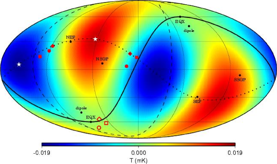
Figure 1: The $\ell=2$ multipole from the Tegmark et al. (2003) cleaned map, presented in Galactic coordinates, after correcting for the kinetic quadrupole. The solid line is the ecliptic plane and the dashed line is the supergalactic plane. The directions of the equinoxes (EQX), dipole due to our motion through the Universe, north and south ecliptic poles (NEP and SEP) and north and south supergalactic poles (NSGP and SSGP) are shown. The multipole vectors are plotted as the solid red (dark gray in gray scale version) symbols for each map, ILC (circles), TOH (diamonds), and LILC (squares). The open symbols of the same shapes are for the normal vector for each map. The dotted line is the great circle connecting the two multipole vectors for this map. The minimum and maximum temperature locations in this multipole are shown as the white stars. The direction that maximizes the angular momentum dispersion of any of the maps coincides with the respective normal vector as discussed in the text.

3.3 Relation to “angular momentum dispersion” axes

The peculiar alignment of the quadrupole and octopole was first pointed out by de Oliveira-Costa et al. (2004). They identified $\hat{\mn@boldsymbol{n}}_{\ell}$ as the axis, which, when chosen as the fiducial $z$-axis of the coordinate system, maximizes the “angular momentum dispersion” of each multipole,

$$(\Delta L)_{\ell}^{2}\equiv\sum_{m=-\ell}^{\ell}m^{2}|a_{\ell m}|^{2}.$$ (19)

By varying the direction of the fiducial $z$-axis over the sky, and recomputing for each such choice the $a_{\ell m}$ and $(\Delta L)_{\ell}^{2}$, they were able to find the choice of $z$-axis that maximizes $(\Delta L)_{\ell}^{2}$. This angular momentum axis distills from each multipole a limited amount of information, reducing the $2\ell$ degrees of freedom in the $\{\hat{\mn@boldsymbol{v}}^{(\ell,j)}\}$ to just two.

Interestingly, de Oliveira-Costa et al. (2004) found that $\hat{\mn@boldsymbol{n}}_{2}\cdot\hat{\mn@boldsymbol{n}}_{3}=0.9838$ in the TOH map. If the $\ell=2$ modes and the $\ell=3$ modes are indeed statistically independent, then this degree of alignment has only a $1.6\%$ chance of happening accidentally. (Arguably this probability should be increased by a factor of two, to $3.2\%$, since we would have been equally surprised if $\hat{\mn@boldsymbol{n}}_{2}$ had been nearly orthogonal to $\hat{\mn@boldsymbol{n}}_{3}$.)

We can calculate $\hat{\mn@boldsymbol{n}}_{2}$ explicitly for the quadrupole in terms of the multipole vectors. The quadrupole function is

$$Q(\mn@boldsymbol{r})=\left(\hat{\mn@boldsymbol{v}}^{(2,1)}\cdot\hat{\mn@boldsymbol{e}}\right)\left(\hat{\mn@boldsymbol{v}}^{(2,2)}\cdot\hat{\mn@boldsymbol{e}}\right)-\frac{1}{3}\hat{\mn@boldsymbol{v}}^{(2,1)}\cdot\hat{\mn@boldsymbol{v}}^{(2,2)},$$ (20)

where $\hat{\mn@boldsymbol{e}}=\mn@boldsymbol{r}/r$. We now apply to $Q(\mn@boldsymbol{r})$ the angular momentum operator

$$\mn@boldsymbol{L}=-\mathrm{i}r\hat{\mn@boldsymbol{e}}\times\mn@boldsymbol{\nabla},$$ (21)

finding

$$-\mathrm{i}\mn@boldsymbol{L}Q=(\hat{\mn@boldsymbol{v}}^{(2,1)}\times\hat{\mn@boldsymbol{e}})(\hat{\mn@boldsymbol{v}}^{(2,2)}\cdot\hat{\mn@boldsymbol{e}})+(\hat{\mn@boldsymbol{v}}^{(2,2)}\times\hat{\mn@boldsymbol{e}})(\hat{\mn@boldsymbol{v}}^{(2,1)}\cdot\hat{\mn@boldsymbol{e}}).$$ (22)

We want to maximize

$$\left(\Delta L\right)_{2}^{2}\equiv\int_{\mathrm{sky}}|{\hat{\mn@boldsymbol{n}}}\cdot{\mn@boldsymbol{L}}Q|^{2}\mathrm{d}{\hat{\mn@boldsymbol{e}}}$$ (23)

over all possible unit vectors to find ${\hat{\mn@boldsymbol{n}}}_{2}$. The quantity $({\hat{\mn@boldsymbol{n}}}\cdot{\mn@boldsymbol{L}}Q)$ is easily calculated:

$$\mathrm{i}{\hat{\mn@boldsymbol{n}}}\cdot{\mn@boldsymbol{L}}Q = \hat{\mn@boldsymbol{e}}\cdot\left[(\hat{\mn@boldsymbol{v}}^{(2,1)}\times{\hat{\mn@boldsymbol{n}}})(\hat{\mn@boldsymbol{v}}^{(2,2)}\cdot{\hat{\mn@boldsymbol{e}}})\right.$$ (24)

$$\quad\left.{}+(\hat{\mn@boldsymbol{v}}^{(2,2)}\times{\hat{\mn@boldsymbol{n}}})(\hat{\mn@boldsymbol{v}}^{(2,1)}\cdot{\hat{\mn@boldsymbol{e}}})\right].$$

The integral in (23) is straightforward in any basis. For an axis

$${\hat{\mn@boldsymbol{n}}}\equiv\left(\sin\chi\cos\psi,\sin\chi\sin\psi,\cos\chi\right),$$ (25)

in a coordinate system where $\hat{\mn@boldsymbol{v}}^{(2,1)}$ is identified with the $x$-axis and $\hat{\mn@boldsymbol{v}}^{(2,2)}$ is taken to define the $xy$-plane with $\hat{\mn@boldsymbol{v}}^{(2,1)}\cdot\hat{\mn@boldsymbol{v}}^{(2,2)}\equiv\cos\omega$,

$$\left(\Delta L\right)_{2}^{2} = \frac{4\pi}{15}\left[4-\sin^{2}\chi\left(2+\sin^{2}\omega+\cos(2\omega-2\psi)\right.\right.$$ (26)

$$\quad\left.\left.{}+\cos(2\psi)\right)\right].$$

The partial derivative of $\left(\Delta L\right)_{2}^{2}$ with respect to $\chi$ vanishes at $\chi=0$, $\pi/2$ and $\pi$. We find that when $\chi=\pi/2$ there are four minima of $\left(\Delta L\right)_{2}^{2}$ for $\psi=\omega/2+n\pi/2$, $n=0,1,2,3$. The directions $\chi=0$ and $\pi$ are maxima. Since $\psi$ is not defined when $\sin\chi=0$, these are zeroes of all directional derivatives. Thus, the “maximum angular dispersion” is obtained in the direction normal to the plane that is defined by the two multipole vectors of the quadrupole, i.e. $\pm(\hat{\mn@boldsymbol{v}}^{(2,1)}\times\hat{\mn@boldsymbol{v}}^{(2,2)})/|\hat{\mn@boldsymbol{v}}^{(2,1)}\times\hat{\mn@boldsymbol{v}}^{(2,2)}|$. The minima are defined by the directions $\pm(\hat{\mn@boldsymbol{v}}^{(2,1)}\pm\hat{\mn@boldsymbol{v}}^{(2,2)})/\sqrt{2}$.

We had previously identified the “area vectors”

$${\mn@boldsymbol{w}}^{(\ell;i,j)}\equiv{\hat{\mn@boldsymbol{v}}}^{(\ell,i)}\times{\hat{\mn@boldsymbol{v}}}^{(\ell,j)}$$ (27)

and the corresponding normalized directions $\hat{\mn@boldsymbol{w}}^{(\ell;i,j)}$ as phenomenologically interesting. Indeed, most of the interesting statistical results of Copi et al. (2004) and Schwarz et al. (2004) relate to statistics of the dot-products of area vectors (or their normalized versions) with one another or with physical directions on the sky, rather than to the statistics of the dot-products of the multipole vectors themselves. We see that for $\ell=2$, the maximum angular momentum dispersion (MAMD) axis is parallel to the area vector, i.e. ${\hat{\mn@boldsymbol{n}}}_{2}=\pm{\hat{\mn@boldsymbol{w}}}^{(2;1,2)}$.

This relation between the area vectors and the MAMD axis cannot extend precisely to higher $\ell$. An octopole, for example, has three multipole vectors $\left\{{\hat{\mn@boldsymbol{v}}}^{(3,i)}\mid i=1,2,3\right\}$ which define three distinct planes with area vectors $\left\{{\mn@boldsymbol{w}}^{(3;i,j)}\mid i,j=1,2,3;i<j\right\}$. The octopole function is

$$\mathcal{O}(\hat{\mn@boldsymbol{e}})=(\hat{\mn@boldsymbol{v}}^{(3,1)}\cdot{\hat{\mn@boldsymbol{e}}})(\hat{\mn@boldsymbol{v}}^{(3,2)}\cdot{\hat{\mn@boldsymbol{e}}})(\hat{\mn@boldsymbol{v}}^{(3,3)}\cdot{\hat{\mn@boldsymbol{e}}})-\mathcal{T}_{3},$$ (28)

where the trace term is

$$\mathcal{T}_{3} = \frac{1}{5}\hat{\mn@boldsymbol{e}}\cdot\left[(\hat{\mn@boldsymbol{v}}^{(3,1)}\cdot\hat{\mn@boldsymbol{v}}^{(3,2)})\hat{\mn@boldsymbol{v}}^{(3,3)}+(\hat{\mn@boldsymbol{v}}^{(3,2)}\cdot\hat{\mn@boldsymbol{v}}^{(3,3)})\hat{\mn@boldsymbol{v}}^{(3,1)}\right.$$ (29)

$$\quad\left.{}+(\hat{\mn@boldsymbol{v}}^{(3,3)}\cdot\hat{\mn@boldsymbol{v}}^{(3,1)})\hat{\mn@boldsymbol{v}}^{(3,2)}\right].$$

Once again, the function $({\hat{\mn@boldsymbol{n}}}\cdot{\mn@boldsymbol{L}}{\cal O})$ is easily calculated for some arbitrary axis $\hat{\mn@boldsymbol{n}}$

$$\mathrm{i}{\hat{\mn@boldsymbol{n}}}\cdot{\mn@boldsymbol{L}}{\cal O} = {\hat{\mn@boldsymbol{e}}}\cdot\left\{\left[(\hat{\mn@boldsymbol{v}}^{(3,1)}\cdot{\hat{\mn@boldsymbol{e}}})(\hat{\mn@boldsymbol{v}}^{(3,2)}\cdot{\hat{\mn@boldsymbol{e}}})\hat{\mn@boldsymbol{v}}^{(3,3)}\right.\right.$$ (30)

$$\left.\left.-\frac{1}{5}(\hat{\mn@boldsymbol{v}}^{(3,1)}\cdot\hat{\mn@boldsymbol{v}}^{(3,2)})\hat{\mn@boldsymbol{v}}^{(3,3)}\right.\right.$$

$$\left.\left.+\mbox{\ cyclic\ permutations}\right]\times{\hat{\mn@boldsymbol{n}}}\right\}.$$

The MAMD axis, ${\hat{\mn@boldsymbol{n}}}_{3}$, is obtained by integrating the square modulus of this function over the full-sky $\mathrm{d}{\hat{\mn@boldsymbol{e}}}$, and maximizing with respect to the choice of axis ${\hat{\mn@boldsymbol{n}}}$. Unlike in the quadrupole case, we don’t find ${\hat{\mn@boldsymbol{n}}}_{3}$ to be a simple combination of the three octopole vectors $\hat{\mn@boldsymbol{v}}^{(3,i)}$. Rather, ${\hat{\mn@boldsymbol{n}}}_{3}$ is some combination of the three directions which is difficult to determine analytically.

In the specific case where the three octopole vectors lie in a plane, (corresponding to a so-called “planar” octopole) the cross product of any two are orthogonal to all three. For a planar octopole, the MAMD axis and the area vectors of the three octopole planes are all parallel. In the case of the observed microwave background, the octopole is relatively planar, for example for the TOH map:

$$|{\mn@boldsymbol{w}}^{(3;1,2)}+{\mn@boldsymbol{w}}^{(3;2,3)}+{\mn@boldsymbol{w}}^{(3;3,1)}|$$ (31)

$$\simeq 0.8\left(|{\mn@boldsymbol{w}}^{(3;1,2)}|+|{\mn@boldsymbol{w}}^{(3;2,3)}|+|{\mn@boldsymbol{w}}^{(3;3,1)}|\right).$$

Moreover, the three octopole area vectors surround the quadrupole area vector (see Fig. 3), so that the MAMD axis — which is some average of the area vectors — is even closer to the quadrupole axis. For these reasons, the MAMD axis is a moderately good representation of the octopole area vectors. This explains that the alignment of the quadrupole and octopole seen by de Oliveira-Costa et al. (2004) and by us (Schwarz et al., 2004) are indeed the same effect.

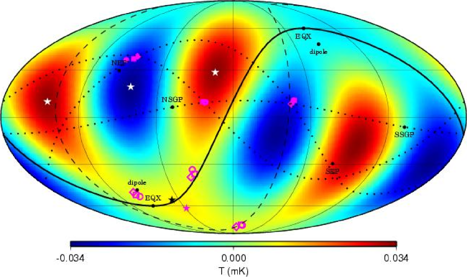
Figure 2: The $\ell=3$ multipole from the Tegmark et al. (2003) cleaned map, presented in Galactic coordinates. The solid line is the ecliptic plane and the dashed line is the supergalactic plane. The directions of the equinoxes (EQX), dipole due to our motion through the Universe, north and south ecliptic poles (NEP and SEP) and north and south supergalactic poles (NSGP and SSGP) are shown. The multipole vectors are the solid magenta (medium gray in gray scale version) symbols for each map, ILC (circles), TOH (diamonds), and LILC (squares). The open symbols of the same shapes are for the normal vectors for each map. The dotted lines are the great circles connecting each pair of multipole vectors for this map. The light gray stars are particular sums of the multipole vectors which are very close to the temperature minima and maxima of the multipole. The solid black star shows the direction of the vector that appears in the trace of the octopole, $\mathcal{T}_{3}$ (29), of the TOH map. The solid magenta (again medium gray in the gray scale version) star is the direction to the maximum angular momentum dispersion for the octopole, again for the TOH map.

3.4 Relation to minima/maxima directions

The directions toward the minima and maxima of each multipole are simple to see and at first glance appear to be an equally useful representation (see Gluck & Pisano 2005). This, however, is not the case.

Consider again the quadrupole (20). The extrema of $Q$ on the sphere occur where the angular momentum is zero. That is, they are the solutions of

$$0 = -\mathrm{i}\mn@boldsymbol{L}Q(\mn@boldsymbol{r})$$ (32)

$$= (\hat{\mn@boldsymbol{v}}^{(2,1)}\times{\hat{\mn@boldsymbol{e}}})(\hat{\mn@boldsymbol{v}}^{(2,2)}\cdot\hat{\mn@boldsymbol{e}})+(\hat{\mn@boldsymbol{v}}^{(2,2)}\times{\hat{\mn@boldsymbol{e}}})(\hat{\mn@boldsymbol{v}}^{(2,1)}\cdot\hat{\mn@boldsymbol{e}}).$$

The solutions of these equations occur (by inspection) along the directions

$$\hat{\mn@boldsymbol{e}}=\hat{\mn@boldsymbol{v}}^{(2,\pm)}\equiv\frac{\hat{\mn@boldsymbol{v}}^{(2,1)}\pm\hat{\mn@boldsymbol{v}}^{(2,2)}}{|\hat{\mn@boldsymbol{v}}^{(2,1)}\pm\hat{\mn@boldsymbol{v}}^{(2,2)}|}=\frac{\hat{\mn@boldsymbol{v}}^{(2,1)}\pm\hat{\mn@boldsymbol{v}}^{(2,2)}}{\sqrt{2(1\pm\hat{\mn@boldsymbol{v}}^{(2,1)}\cdot\hat{\mn@boldsymbol{v}}^{(2,2)})}}$$ (33)

It is easily seen that $\hat{\mn@boldsymbol{v}}^{(2,+)}\cdot\hat{\mn@boldsymbol{v}}^{(2,-)}=0$. Thus we see that for the quadrupole the maxima and minima are orthogonal to each other and lie in the same plane as the multipole vectors. The quadrupole multipole vectors bracket the two hot spots — the maxima occur half way between the two multipole vectors.

The quadrupole multipole vectors $\hat{\mn@boldsymbol{v}}^{(2,1)}$ and $\hat{\mn@boldsymbol{v}}^{(2,2)}$ contain 4 pieces of information and thus fully specify the shape of the quadrupole (the fifth piece of information being the amplitude $A^{(2)}$). The same is not true of the ${\hat{\mn@boldsymbol{v}}}^{(2,\pm)}$, the directions to the maxima and minima. Since the minima and maxima are orthogonal, these vectors contain only three pieces of information — for example, the direction of the first maximum, and the orientation of the plane of the maxima and minima. The ratio of the amplitudes of the two maxima and minima is unspecified. That is, we do not know the relative strengths of the maxima and minima.

For higher multipoles the minima/maxima directions, unlike the multipole vectors, persist in not containing the full information. The minima and maxima directions will again lack information about the relative amplitude of the extrema. There are also additional problems concerning the definition of the minima/maxima directions: In the case of a pure $Y_{\ell 0}$ mode, there are degenerate rings of minima/maxima, which do not allow to assign a unique direction. Moreover, the number of minima and maxima for a fixed value of $\ell$ is not unique. For a pure mode (spherical harmonic) the number of extrema depends on $\ell$ and $m$ in general. To see that it is instructive to remember that $\ell$ corresponds to the total number of nodal lines and $m$ counts the number of meridians that are nodal lines. With this rule in mind one can easily see that, e.g. $Y_{32}$ has four maxima and four minima, whereas $Y_{33}$ has three maxima and three minima. For a general multipole there is no rule on how many minima and maxima we should expect and thus the minimum/maximum directions are only of limited use. Conversely, multipole vectors always contain $2\ell$ pieces of information, including information on the location, number and relative amplitudes of the minima and maxima.

Therefore, while one might have at first imagined the minima/maxima directions to be independent, they are actually strongly correlated. This weakens the statistical power of tests of the distribution of these directions. For these reasons, the statistical properties of the minima/maxima directions are not considered further in this work.

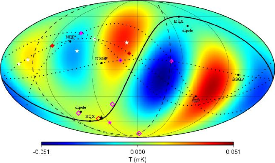
Figure 3: The $\ell=2+3$ multipoles from the Tegmark et al. (2003) cleaned map, presented in Galactic coordinates. This is a combination of Figs. 1 and 2 with only the multipole vectors for the TOH map shown for clarity. The solid line is the ecliptic plane and the dashed line is the supergalactic plane. The directions of the equinoxes (EQX), dipole due to our motion through the Universe, north and south ecliptic poles (NEP and SEP) and north and south supergalactic poles (NSGP and SSGP) are shown. The $\ell=2$ multipole vectors are plotted as the solid red (dark gray in gray scale version) diamond and their normal is the open red (dark gray in the gray scale version) diamond. The $\ell=3$ multipole vectors are the solid magenta (medium gray in gray scale version) diamonds and their three normals are the open magenta (medium gray in the gray scale version) diamonds. The dotted lines are the great circles connecting the multipole vectors for this map (one for the quadrupole vectors and three for the octopole vectors). The minimum and maximum temperature locations of the $\ell=2$ multipole are shown as the white stars. The light gray stars are particular sums of the $\ell=3$ multipole vectors which are very close to the temperature minima and maxima of the octopole. The solid black star shows the direction of the vector that appears in the trace of the octopole, $\mathcal{T}_{3}$ (29). The solid magenta (again medium gray in the gray scale version) star is the direction to the maximum angular momentum dispersion for the octopole, again for the TOH map.

3.5 Relation to Land-Magueijo vectors

Magueijo (1995) discussed an alternative approach to the $\ell$-th multipole, which is well known to be a representation of a symmetric trace-free tensor of rank $\ell$. Much as for the multipole vectors, in this approach one recasts the $\ell$-th multipole as a $3\times 3\times\cdots\times 3$ ($\ell$ dimensional) Cartesian tensor, ${\cal O}^{i_{1}\cdots i_{\ell}}$ (with $i_{n}=1,2,3$). One then realizes that the information this Cartesian tensor encodes can be recast as $2\ell-2$ scalars, the $2\ell-2$ independent invariant contractions of the rank $\ell$ trace-free symmetric tensor, and three degrees of freedom associated with an orthonormal frame. (The orientation of the $z$-axis of the frame is two degrees of freedom. The orientation of the $x$-axis within the plane orthogonal to the $z$-axis is the third. The $y$-axis is then fixed by orthonormality and the convention of right-handedness.)

Land & Magueijo (2005b) discussed the two scalars and the frame associated with the microwave background quadrupole. The two scalars are the power-spectrum and the bispectrum. The vectors of the frame are the eigenvectors of the $3\times 3$ Cartesian quadrupole tensor. This has the advantage that, at least for the quadrupole, one has clearly separated the issue of non-Gaussianity (the bispectrum) from that of statistical anisotropy (the frame). Land and Magueijo claimed that the frame they found was independent of the multipole vectors described in Schwarz et al. (2004). However, Schwarz and Starkman (private communication, 2004 as referenced in Land & Magueijo 2005d) showed that, in fact, two of the axes of the frame are parallel to the sum and difference of the quadrupole multipole vectors $\hat{\mn@boldsymbol{v}}^{(2,1)}\pm\hat{\mn@boldsymbol{v}}^{(2,2)}$. The third is, of course, parallel to their cross-product.

Explicitly, for a quadrupole with multipole vectors $\hat{\mn@boldsymbol{v}}^{(2,1)}$ and $\hat{\mn@boldsymbol{v}}^{(2,2)}$, the Cartesian tensor representation of the quadrupole (20) is

$${\cal Q}_{ij}=\frac{{\hat{\mn@boldsymbol{v}}^{(2,1)}}_{i}{\hat{\mn@boldsymbol{v}}^{(2,2)}}_{j}+{\hat{\mn@boldsymbol{v}}^{(2,1)}}_{j}{\hat{\mn@boldsymbol{v}}^{(2,2)}}_{i}}{2}-\frac{1}{3}{\hat{\mn@boldsymbol{v}}^{(2,1)}}\cdot{\hat{\mn@boldsymbol{v}}^{(2,2)}}\delta_{ij}.$$ (34)

This $3\times 3$ matrix can be diagonalized. The three eigenvectors making up the Land and Magueijo orthonormal frame are

$$\mn@boldsymbol{v}^{(\mathrm{LM})}_{1} \parallel \hat{\mn@boldsymbol{v}}^{(2,1)}\times\hat{\mn@boldsymbol{v}}^{(2,2)}$$

$$\mn@boldsymbol{v}^{(\mathrm{LM})}_{2} \parallel \hat{\mn@boldsymbol{v}}^{(2,1)}+\hat{\mn@boldsymbol{v}}^{(2,2)}$$ (35)

$$\mn@boldsymbol{v}^{(\mathrm{LM})}_{3} \parallel \hat{\mn@boldsymbol{v}}^{(2,1)}-\hat{\mn@boldsymbol{v}}^{(2,2)}.$$

It is noteworthy that $\mn@boldsymbol{v}^{(\mathrm{LM})}_{2}$ and $\mn@boldsymbol{v}^{(\mathrm{LM})}_{3}$ are in the directions of the quadrupole maxima (or minima), while $\mn@boldsymbol{v}_{1}^{(\mathrm{LM})}$ is the quadrupole area vector $\mn@boldsymbol{w}^{(2;1,2)}$. (The claim by Land & Magueijo (2005b) that these vectors did not coincide with the quadrupole multipole vectors or area vector of Schwarz et al. (2004) arose because Schwarz et al. (2004) corrected for the kinetic quadrupole as discussed in Sec. 2.4).

A difficulty that arises with the Land and Magueijo approach is how to go beyond the quadrupole. Land & Magueijo (2005d) note that the $2\ell-2$ independent scalars associated with the $\ell$-th multipole are just the $2\ell-2$ linearly independent combinations of dot-products of the $\ell$ multipole vectors. The orthonormal frame is then constructed out of the multipole vectors, as they were for the quadrupole. However, there are $\ell$ multipole vectors and so $\ell(\ell-1)$ different ways to construct the frame (not to mention a much larger number of ways to choose the set of independent scalars). To define a unique orthonormal frame Land & Magueijo (2005e) chose the two vectors that have the two largest values of

$$K_{i}=\sum_{j\neq i}\left(\hat{\mn@boldsymbol{v}}_{i}\cdot\hat{\mn@boldsymbol{v}}_{j}\right)^{2}.$$ (36)

This is not a unique choice and it is unclear how to fairly choose such a frame. When they claim that it is this orthonormal frame that one should use to test statistical isotropy, we must ask which of the many possible allowed choices of frame is the correct one. As Land & Magueijo (2005e) point out the choice of frame is crucial and their scheme is increasingly sensitive to small fluctuations in the positions of the multipole vectors as $\ell$ grows. This leads to discontinuous noise in the Euler angles of the orthogonal frame making it difficult to interpret the results. As Land & Magueijo (2005e) also point out different orderings of the vectors will be sensitive to different features in the data. Without a unique and well understood prescription this approach does not lead to further understanding. The multipole vectors, on the other hand are unique. It is true, as Copi et al. (2004) and Schwarz et al. (2004) point out, and as reiterated by Land & Magueijo (2005d), that they contain information on both statistical isotropy and non-Gaussianity. Optimal separation of these two properties remains an open problem.

3.6 Polydipoles

The directions of the multipole vectors are somewhat difficult to interpret physically. We would argue that in large measure this is due to the removal of the traces done in constructing the multipole vector expansion (9). An alternative approach would be to write the general function $f(\theta,\phi)$ in a slightly different way:

$$f(\theta,\phi)=\sum_{\ell=0}^{\infty}{\cal P}_{\ell}(\theta,\phi)\equiv\sum_{\ell=0}^{\infty}A_{\rm P}^{(\ell)}\prod_{i=1}^{\ell}({\hat{\mn@boldsymbol{p}}}^{(\ell,i)}\cdot{\hat{\mn@boldsymbol{e}}}).$$ (37)

The ${\cal P}_{\ell}$’s, which we term polydipoles, are similar to the multipoles $f_{\ell}$ in equation (9), except for our failure to remove the traces in their construction. But it is this failure which makes them easily visualized: ${\cal P}_{\ell}(\theta,\phi)$ is the simple product of $\ell$ dipoles. Therefore there are $\ell$ great circles on which ${\cal P}_{\ell}(\theta,\phi)$ vanishes — the great circles are normal to each of the polydipole vectors ${\hat{\mn@boldsymbol{p}}}^{(\ell,i)}$. These are clearly related to the $\ell$ nodal curves of $Y_{\ell m}$.

Unfortunately the polydipole expansion (37) is unstable in the following important sense. Suppose that in expanding $f(\theta,\phi)$ we at first neglect all contributions with angular momentum greater than $L$ and calculate $f_{\ell}$ and ${\cal P}_{\ell}$ for $\ell=1,\ldots,L$. If we then increase $L$, the $f_{\ell}$’s do not change (since the spherical harmonics are an orthogonal basis) but the ${\cal P}_{\ell}$ generally do. Thus, the polydipole expansion is well-defined only if the angular power spectrum falls sufficiently quickly at large $\ell$. The precise condition for convergence of the polydipole expansion has not been determined.

The “leading” term in a multipole $f_{\ell}$ (by which we mean the part excluding ${\cal T}_{\ell}$ in (9)) is a polydipole, which we may term the associated polydipole of that multipole. (Note that the multipole vectors are not however the vectors one would get in the polydipole expansion, so the $\ell$th polydipole in a polydipole expansion is not the associated polydipole of the $\ell$th multipole in a multipole expansion.) To the extent that it is easier to visualize the polydipole, it is of some limited interest.

4 The Strange Properties of the Quadrupole and the Octopole

As we have already remarked, the microwave background anisotropies on large angular scales seem to have several unusual properties. Most widely known is that the power in the quadrupole, $C_{2}$, is substantially less than is expected from the models that fit the rest of the angular power spectrum (and other) data. The power in the octopole is also less than expected, though within cosmic variance error bars. By $\ell=4$ the power in the CMB is entirely consistent with theoretical expectations. This was first found by COBE (Bennett et al., 1996) and has now been confirmed by WMAP. The precise statistical significance of this deviation is a matter of some dispute (Efstathiou, 2004; Slosar et al., 2004; Bielewicz et al., 2004; O’Dwyer et al., 2004).

It has also been known since COBE, but had largely been forgotten until confirmed by WMAP (Spergel et al., 2003), that the two-point angular correlation function of the microwave background

$$C(\theta)=\langle T(\hat{\mn@boldsymbol{e}}_{1})T(\hat{\mn@boldsymbol{e}}_{2})\rangle$$ (38)

(where $\hat{\mn@boldsymbol{e}}_{1}\cdot\hat{\mn@boldsymbol{e}}_{2}=\cos\theta$) is nearly zero at angular scales between about $60\degr$ and $170\degr$. Spergel et al. (2003) argued that, given the best fitting $\Lambda$CDM model, this is unlikely at the $0.15$% level. What has been under-appreciated, is that this vanishing of $C(\theta)$ is not merely due to the lack of quadrupole power, but also due to the lack of octopole power, and maybe even to the ratio of $C_{2}:C_{3}:C_{4}$ (Luminet et al., 2003).

These anomalies relate exclusively to the power in the various multipoles. More recently, attention has turned to the “shapes”, “phase relationships” or “orientations” of the multipoles, i.e. to the information contained in the multipole vectors. As remarked above, several groups of authors have noticed particular anomalies. In this section, we will first describe them, mostly in the language of multipole vectors, before proceeding to try to assign them some statistical significance in the next section.

We believe that the observed lack of power at large angles justifies singling out the two most responsible multipoles for particular scrutiny. To do so is no more dubious than the practice of firefighters to respond to the house where the fire alarm is ringing rather than to all the houses in the neighborhood. That these lowest multipoles represent a physically interesting scale — the recent scale of the horizon, especially the scale of the horizon at approximately dark energy domination — makes it doubly justified to focus our attention, at least initially, on them.

Table 1 contains the multipole vectors and area vectors for the quadrupole and octopole that will be discussed below.

Table 1: Multipole vectors, $\hat{\mn@boldsymbol{v}}^{(\ell,i)}$, and oriented area vectors, $\mn@boldsymbol{w}^{(\ell;i,j)}$, for the quadrupole and octopole in Galactic coordinates $(l,b)$. All vectors are given for the TOH cleaned map after correcting for the kinetic quadrupole and the coordinates are consistent with how they are plotted in Figs. 1–3 and 6. The magnitudes for the oriented area vectors are also given.

Vector	$l$		$b$		Magnitude
$\hat{\mn@boldsymbol{v}}^{(2,1)}$	$118$$\aas@@fstack{\circ}$	$9$	$25$$\aas@@fstack{\circ}$	$1$	—
$\hat{\mn@boldsymbol{v}}^{(2,2)}$	$11$$\aas@@fstack{\circ}$	$2$	$16$$\aas@@fstack{\circ}$	$6$	—
$\mn@boldsymbol{w}^{(2;1,2)}$	$74$$\aas@@fstack{\circ}$	$3$	$-56$$\aas@@fstack{\circ}$	$6$	0.990
$\hat{\mn@boldsymbol{v}}^{(3,1)}$	$86$$\aas@@fstack{\circ}$	$9$	$39$$\aas@@fstack{\circ}$	$3$	—
$\hat{\mn@boldsymbol{v}}^{(3,2)}$	$22$$\aas@@fstack{\circ}$	$6$	$9$$\aas@@fstack{\circ}$	$2$	—
$\hat{\mn@boldsymbol{v}}^{(3,3)}$	$-44$$\aas@@fstack{\circ}$	$9$	$8$$\aas@@fstack{\circ}$	$2$	—
$\mn@boldsymbol{w}^{(3;1,2)}$	$101$$\aas@@fstack{\circ}$	$6$	$-49$$\aas@@fstack{\circ}$	$8$	0.902
$\mn@boldsymbol{w}^{(3;2,3)}$	$-6$$\aas@@fstack{\circ}$	$3$	$-79$$\aas@@fstack{\circ}$	$5$	0.918
$\mn@boldsymbol{w}^{(3;3,1)}$	$38$$\aas@@fstack{\circ}$	$4$	$-38$$\aas@@fstack{\circ}$	$9$	0.907

4.1 The queerness of the quadrupole

Figure 1 shows the $\ell=2$ multipole from the Tegmark et al. (2003) cleaned map after subtraction of the kinetic quadrupole. The solid line is the ecliptic plane and the dashed line is the supergalactic plane. The directions of the equinoxes (EQX), dipole due to our motion through the Universe, north and south ecliptic poles (NEP and SEP) and north and south supergalactic poles (NSGP and SSGP) are shown. The multipole vectors are plotted as the solid red symbols for each map (see figure caption), while the open symbols of the same shapes are for the normal vector for each map. The dotted line is the great circle connecting the two multipole vectors for this map. The minimum and maximum locations of the temperature in this multipole are shown as the white stars. The following observations can be made about the quadrupole:

1. The great circle defined by the quadrupole multipole vectors $\hat{\mn@boldsymbol{v}}^{(2,1)}$ and $\hat{\mn@boldsymbol{v}}^{(2,2)}$ passes through the NEP and SEP. This is especially true for the TOH and LILC maps, with some slight deviation for the ILC map. We can rephrase this to say that the (normalized) quadrupole area vector $\hat{\mn@boldsymbol{w}}^{(2;1,2)}$ lies on the ecliptic plane.

2. The axis of this great circle (i.e., $\hat{\mn@boldsymbol{w}}^{(2;1,2)}$) is aligned with both the dipole and the equinoxes.

4.2 The oddness of the octopole

Figure 2 shows the $\ell=3$ multipole from the Tegmark et al. (2003) cleaned map. Many of the features are the same as for the quadrupole map (see Fig. 1). Note that there are now 3 multipole vectors (closed symbols) and 3 normal vectors (open symbols) plotted. Also there are 3 dotted lines showing the great circles connecting each pair of multipole vectors for this map. Several perplexing observations can also be made about the properties of the octopole.

1. The octopole has three multipole vectors: $\hat{\mn@boldsymbol{v}}^{(3,1)}$, $\hat{\mn@boldsymbol{v}}^{(3,2)}$ and $\hat{\mn@boldsymbol{v}}^{(3,3)}$. One of these, $\hat{\mn@boldsymbol{v}}^{(3,1)}$, lies quite near the ecliptic poles. Therefore, the two great circles defined by the pairs $(\hat{\mn@boldsymbol{v}}^{(3,1)},\hat{\mn@boldsymbol{v}}^{(3,2)})$ and the pair $(\hat{\mn@boldsymbol{v}}^{(3,1)},\hat{\mn@boldsymbol{v}}^{(3,3)})$ each nearly pass through the ecliptic poles. But in fact, one of these great circles passes much closer to the poles than the position of $\hat{\mn@boldsymbol{v}}^{(3,1)}$. The associated area vectors, $\mn@boldsymbol{w}^{(3;1,2)}$ and $\mn@boldsymbol{w}^{(3;3,1)}$, therefore lie on (or nearly on) the ecliptic.

2. The third pair of multipole vectors, $(\hat{\mn@boldsymbol{v}}^{(3,2)},\hat{\mn@boldsymbol{v}}^{(3,3)})$ define a great circle that includes the supergalactic poles. This pair also lies within $9\degr$ of the Galactic plane. The associated area vector $\mn@boldsymbol{w}^{(3;2,3)}$, therefore lies on the supergalactic plane and only $10\aas@@fstack{\circ}5$ from the Galactic poles.

3. The octopole is noticeably planar, but not overwhelmingly so. Namely, the area vectors of the octopole cluster only somewhat compared to expectations.

4. The three maxima and three minima are very nearly at $\pm\hat{\mn@boldsymbol{v}}^{(3,1)}\pm\hat{\mn@boldsymbol{v}}^{(3,2)}\pm\hat{\mn@boldsymbol{v}}^{(3,3)}$, even though these are not generically where the angular momentum is zero. (Note that there are 8 such choices but only 6 are either minima or maxima direction.) This contrasts with the quadrupole, where the extrema can be shown analytically to be at $\pm\hat{\mn@boldsymbol{v}}^{(2,1)}\pm\hat{\mn@boldsymbol{v}}^{(2,2)}$ (see section 3.4).

5. The vector from the octopole trace, $\mathcal{T}_{3}$, (see Eqn. 29) lies on the ecliptic plane. The importance of this vector is unclear. Note that $\mathcal{T}_{3}$ is proportional to the difference between the octopole and the polydipole, $\mathcal{P}_{3}$.

4.3 The remarkable relation of the quadrupole and the octopole

Figure 3 shows the sum of $\ell=2$ and $\ell=3$ in the TOH cleaned map, after kinetic quadrupole subtraction. We can see that, beyond the separate oddities of $\ell=2$ and $\ell=3$, there are additional unexpected relationships between the quadrupole and octopole:

1. The quadrupole normal vector $\hat{\mn@boldsymbol{w}}^{(2;1,2)}$ (open red symbols) — or equivalently the quadrupole MAMD axis $\hat{\mn@boldsymbol{n}}_{2}$ — is aligned with the octopole MAMD axis $\hat{\mn@boldsymbol{n}}_{3}$ (magenta star). It is also aligned with the three octopole area vectors (open magenta symbols), especially with one of them.

2. The ecliptic carefully traces a zero of the combined map, doing so almost perfectly over the entire hemisphere centered on the Galactic center, and even relatively well over the antipodal hemisphere.

3. Two of the extrema south of the ecliptic are clearly stronger than any north of the ecliptic. The weakest southern extremum is essentially equal in power to the strongest northern extremum. (It is slightly stronger in the LILC map, slightly weaker in the TOH and ILC maps.)

5 Statistics

We now revisit the statistics used to quantify the alignment of the various vectors with each other and with the Solar System. In Schwarz et al. (2004), we considered the dot-products, $A_{i}$, of the three octopole area vectors with the quadrupole area vector, and the mutual dot-products, $D_{i}$, of the three octopole normal vectors (area vectors normalized to unit length) with the quadrupole normal vector. We found that both the $A_{i}$ and the $D_{i}$ are unusually large. Note that we can take as a convention that $A_{i}\geq 0$ since each vector is ambiguous in sign. The various dot-products are shown in Table 2. As we emphasized in Schwarz et al. (2004), all of the aforementioned alignments are statistically significant at 99.8% C.L. or higher.

To compute all probabilities we compare statistics applied to WMAP maps to that applied to Monte Carlo simulations. Unless otherwise noted, Monte Carlo simulations are comprised of 100,000 realizations of Gaussian random, statistically isotropic maps with WMAP’s (inhomogeneous) pixel noise.

Table 2: Values of various vector dot-products for the TOH cleaned map, corrected for the kinetic quadrupole. We show the values of the dot-products of the three octopole area vectors with the quadrupole area vector ($A_{i}$, $i=1,2,3$); the dot-products of the three octopole normal vectors with the quadrupole normal vector ($D_{i}$, $i=1,2,3$; the normals are the unit area vectors); and the dot-products of the four quadrupole and octopole area and normal vectors with the north ecliptic pole (NEP), the north Galactic pole (NGP), the north supergalactic pole (NSGP), the dipole and the equinox.

	Value of the dot-product
Test	${\mn@boldsymbol{w}}^{(2;1,2)}$	${\mn@boldsymbol{w}}^{(3;1,2)}$	${\mn@boldsymbol{w}}^{(3;1,3)}$	${\mn@boldsymbol{w}}^{(3;2,3)}$
$A_{i}$	—	0.851	0.783	0.762
$\mn@boldsymbol{w}\cdot\mathrm{NEP}$	0.027	0.161	0.041	0.481
$\mn@boldsymbol{w}\cdot\mathrm{NGP}$	0.827	0.688	0.570	0.903
$\mn@boldsymbol{w}\cdot\mathrm{NSGP}$	0.392	0.262	0.630	0.0011
$\mn@boldsymbol{w}\cdot\mathrm{dipole}$	0.974	0.883	0.755	0.674
$\mn@boldsymbol{w}\cdot\mathrm{equinox}$	0.968	0.886	0.681	0.766
$D_{i}$	—	0.953	0.872	0.838
$\hat{\mn@boldsymbol{w}}\cdot\mathrm{NEP}$	0.027	0.179	0.045	0.523
$\hat{\mn@boldsymbol{w}}\cdot\mathrm{NGP}$	0.835	0.763	0.629	0.983
$\hat{\mn@boldsymbol{w}}\cdot\mathrm{NSGP}$	0.396	0.291	0.694	0.0012
$\hat{\mn@boldsymbol{w}}\cdot\mathrm{dipole}$	0.984	0.979	0.832	0.733
$\hat{\mn@boldsymbol{w}}\cdot\mathrm{equinox}$	0.978	0.982	0.751	0.834

5.1 Requirements for robust statistics

In previous work (Schwarz et al., 2004), we used a particular set of statistics, for example, for a set of vectors that have dot-products $\{A_{i}\mid i=1,\ldots,n\}$ (with one another, or with a particular physical direction on the sky) with “unusually” high values. We asked what is the probability that a random Monte Carlo map has the highest dot-product higher than $A_{1}$, the second highest one higher than $A_{2}$, the third highest one higher than $A_{3}$, and so on down to the $n\mbox{-}th$ such dot product. For several cases that number was, as reported, very small. For example, for the dot products between the quadrupole area vector $\mn@boldsymbol{w}^{(2;1,2)}$, and each of the three octopole area vectors $\left\{\mn@boldsymbol{w}^{(3;1,2)},\mn@boldsymbol{w}^{(3;2,3)},\mn@boldsymbol{w}^{(3;3,1)}\right\}$, only 21 out of 100,000 MC maps (for the TOH DQ-corrected map) satisfied the criterion, i.e. only 21 had $A_{1}$ larger than the TOH value of $A_{1}$, $A_{2}$ larger than the TOH value of $A_{2}$ and $A_{3}$ larger than the TOH value of $A_{3}$.

One can ask if this statistic preferentially returns a small probability even if there is really none to be found. This is clearly not the case — the vector dot-products could have been either large, small or “average”; we noticed they were large and found an easy to understand statistic that quantified the effect. Weeks (private communication) however has pointed out that the above-described statistics for the $A_{i}$ do not define an ordering relation on the set of possible $A_{i}$; they therefore implicitly incorporate some a posteriori knowledge. One would therefore like to confirm this result with different, independent statistics.

5.2 S and T statistics — definitions

To quantify the various alignments we found, it is desirable to choose the statistics in such a way that the a posteriori knowledge of the particular nature of the alignments is not used to find unjustly small probabilities. With that in mind we define and discuss two statistics, $S$ and $T$, which do define ordering relations. The first of these was briefly mentioned and used in Schwarz et al. (2004) as suggested by Weeks.

Two natural choices of statistics which define ordering relations on the three dot-products $A_{i}$, each lying in the interval $[0,1]$, are:

$$S \equiv {1\over 3}\left(A_{1}+A_{2}+A_{3}\right)$$ (39)

$${\rm and}$$

$$T \equiv 1-{1\over 3}\left[(1-A_{1})^{2}+(1-A_{2})^{2}+(1-A_{3})^{2}\right].$$ (40)

Both $S$ and $T$ can be viewed as the suitably defined “distance” to the vertex $(A_{1},A_{2},A_{3})=(0,0,0)$. A third obvious choice, $(A_{1}^{2}+A_{2}^{2}+A_{3}^{2})/3$, is just $2S-T$. Of course many other choices exist, involving higher powers of $A_{i}$.

One could also ask about the probability that, for example, two out of three normals are aligned, and so we generalize the definitions to

$$S^{(n,m)} \equiv {1\over m}\sum_{i=1}^{m}A_{i}$$ (41)

$$T^{(n,m)} \equiv 1-{1\over m}\sum_{i=1}^{m}(1-A_{i})^{2},$$ (42)

where the $A_{i}$ are ordered from largest to smallest Note that, if the $A_{i}$ are large (near $1$), both $S^{(n,m)}$ and $T^{(n,m)}$ will be large (near $1$).

One could further generalize these statistics to arbitrary weighting by different alignments; for example

$$S^{(n;\mn@boldsymbol{\alpha})}\equiv\left.\sum_{i=1}^{n}\alpha_{i}A_{i}\right/\sum_{i=1}^{n}\alpha_{i}$$ (43)

with $0\leq\alpha_{i}\leq 1$. Hereafter we consider only the values $\alpha_{i}=0$ or $1$. Finally, there is nothing special about the area vector products $A_{i}$ and we apply the statistics $S^{(n,m)}$ to dot-products of the vector normals, $D_{i}$, and also to dot-products of the normals with specific directions or planes in the sky (ecliptic plane, NGP, supergalactic plane, dipole and equinox) that were discussed in Schwarz et al. (2004). When comparing to planes, we order the dot products (taken with the plane’s axis), from smallest to largest.

5.3 S and T statistics — quadrupole and octopole

Figure 4 shows histograms of $S^{(n,m)}$ statistics (left column) and $T^{(n,m)}$ statistics (right column) for Gaussian random, statistically isotropic MC maps, as well as values for the TOH DQ-corrected map. The statistics shown are $S^{(3,m)}$ and $T^{(3,m)}$ for the intrinsic alignment of the octopole area vectors with the quadrupole area vector, and $S^{(4,m)}$ and $T^{(4,m)}$ for the alignment of normals with the ecliptic plane, Galactic poles, and supergalactic plane. The dipole and equinox alignments are similar to the ecliptic plane and are not shown.

Note several interesting features in Fig. 4. First, the probabilities for the algebraically-related values of $S^{(n,1)}$ and $T^{(n,1)}$ are by definition identical, since they measure the extremeness of a single parameter. Second, evidence for alignment of the quadrupole and octopole and for alignment of multipoles with the ecliptic plane (and similarly with the dipole and equinoxes) is strongest when all dot-products are considered — i.e. when $m=n$. This gives us further confidence that these probabilities are generally not dominated by one or two unusual alignments, but rather when alignment of all four normals, either mutual or with the specified direction, are considered.

We note that the alignment of normals with either the supergalactic plane or the Galactic poles is dominated by a single normal, $\hat{\mn@boldsymbol{w}}^{(3;2,3)}$. In the case of the supergalactic plane, this normal is only $0\aas@@fstack{\circ}07$ away from the plane (in the TOH map), while the other three are not particularly close to the plane at all; see Table 2, Figure 1 and Schwarz et al. (2004). Therefore $S^{(4,1)}<S^{(4,m)}$ for $m\geq 2$. Although this normal is still within approximately $1\aas@@fstack{\circ}5$ in the ILC and LILC maps, this is still sufficient to raise the probability of $S^{(4,1)}$ to approximately $10$%. The fact that only the $S^{(4,1)}$ statistic and only the TOH map show small probabilities suggests that the supergalactic correlation is a statistical fluctuation.

The same normal $\hat{\mn@boldsymbol{w}}^{(3;2,3)}$ is approximately $10\degr$ from the Galactic pole. This is largely responsible for the measured correlation of the quadrupole and octopole with the Galactic pole, although it is true that $S^{(4,4)}<S^{(4,1)}$ for this case. We discuss this further in Sec. 5.4.

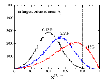
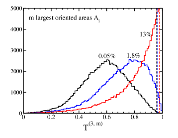
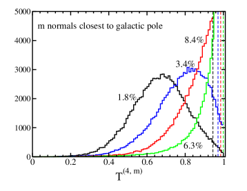
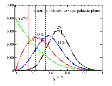
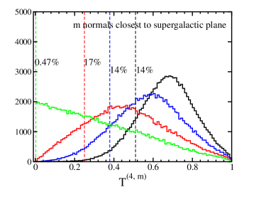
Figure 4: Histograms of $S^{(n,m)}$ statistics (left column) and $T^{(n,m)}$ statistics (right column) for Gaussian random, statistically isotropic Monte Carlo maps with $m=1\ldots n$ of the most aligned area vectors considered separately in each panel. First row panels show the $n=3$ mutual dot-products of quadrupole and octopole area vectors $A_{i}$, second row shows dot-products of the $n=4$ normals with the ecliptic plane, third row shows dot-products of the $n=4$ normals with the north Galactic pole while the fourth row shows dot-products of the $n=4$ normals with the supergalactic plane. Specific values for the WMAP (TOH DQ-corrected map), for each $m$, are shown with vertical lines. The numbers show the percentage of MC maps that have a more extreme value (i.e. larger mutual dot-products $A_{i}$, larger products with the NGP, or smaller dot-products with the NEP and NSGP). In other words, the numbers show the extremeness of each vertical line’s value in the corresponding histogram. Note that the statistical significance is strongest when all vectors are considered (that is, when $m=n$), except for the supergalactic plane where a single octopole normal is only $0\aas@@fstack{\circ}07$ away from this plane while the other three are not particularly unusual.

Table 3: Table of probabilities (in percent) for the seven different tests using the TOH, LILC and ILC maps. We show the results based on both DQ-corrected and uncorrected maps. The statistics $S^{(n,n)}$, computed for each microwave background map and compared to 100,000 realizations of Gaussian random, statistically isotropic maps with WMAP’s pixel noise, has been used to compute all probabilities. Except for the test $D_{i}$, all tests are based on the dot-products of the area vectors, $\mn@boldsymbol{w}$, of the quadrupole and octopole.

Test	TOH DQ-corr	LILC DQ-corr	ILC DQ-corr	TOH uncorr	LILC uncorr	ILC uncorr
$A_{i}$	0.117	0.602	0.289	0.582	2.622	0.713
$D_{i}$	1.246	1.309	2.240	1.262	1.309	2.567
ecliptic plane	1.425	1.480	2.006	1.228	1.735	2.724
NGP	0.734	0.940	0.508	0.909	1.265	0.497
SG plane	14.4	13.4	8.9	11.6	10.2	6.5
dipole	0.045	0.214	0.110	0.093	0.431	0.207
equinox	0.031	0.167	0.055	0.064	0.315	0.080

In the absence of any model, $S^{(n,n)}$ and $T^{(n,n)}$ statistics seem the fairest choice, and the one we adopt. These statistics treat planes and directions identically (i.e. the ordering of the relevant dot-products does not matter). Table 3 shows the probabilities for the seven different tests applied on the TOH, LILC and ILC maps using the $S^{(4,4)}$ statistic. We show the results based on both DQ-corrected and DQ-uncorrected maps.

Finally, there has been some confusion regarding constraints from the application of the $S$ statistic to the normalized, $D_{i}$, and unnormalized, $A_{i}$, area vectors. It has been claimed that the $S$ statistic applied to the area vectors $A_{i}$ is both not a measure of alignment between the octopole and quadrupole and not a very robust statistic. It was argued that one should only use the $D_{i}$. The heuristic argument is that $S$ applied to the $A_{i}$ is not actually a measure of alignment since the $A_{i}$ incorporate information about the lengths of the area vectors, not just their directions (see, for example, Weeks 2004). However, what this means is that the $S$ statistic applied to the $A_{i}$ weights the contribution of each plane according to how well the two associated multipole vectors define that plane — the closer they are to orthogonal, the more well defined the plane is, and the more heavily the plane is weighted; the more nearly parallel they are, the less well defined the plane is and the smaller its weighting in the statistic. This weighting thus seems entirely intuitive and appropriate.

The confusion noted above has arisen from inconsistently applying the test to maps, some with the kinetic quadrupole correction applied and others without it. The specific concern about the robustness of this statistical test was that the $S$ statistic applied to the $A_{i}$ of the LILC map was apparently much less unlikely than the $S$ statistic applied to the $A_{i}$ of the TOH map (Weeks, 2004). However, this result compared the Doppler-corrected TOH map to the uncorrected LILC map. The former has probability around $0.1\%$, whereas the latter has probability $2.6\%$. When we Doppler-correct the LILC map (as one should), we find that the probability falls to around $0.6\%$, comparable to that of the TOH map (see Table 3). Also the Doppler corrected ILC map yields a similar $0.2\%$ probability. Far from challenging the robustness of the $S$ statistic for the area vectors, the probabilities derived from different maps support it.

5.4 The evidence for ecliptic (and other) alignment

The values in Table 3 show alignment of the area vectors of the quadrupole and octopole with each other and with some specific physical directions. Also shown in Table 3 is the statistical evidence for a correlation with the dipole and equinox direction (at larger $99.7\%$C.L. in all three maps), with the NGP (at larger $99\%$C.L.) and the ecliptic plane (at larger $98\%$C.L.). As discussed in Sec. 5.3, our use of the $S^{(4,4)}$ statistic (instead of the $S^{(4,1)}$ statistic) shows that the correlation with the supergalactic plane is not significant.

Previously we have claimed that there is evidence for ecliptic alignment, but not for Galactic alignment. Yet Table 3 shows a slightly higher significance for the Galactic than the ecliptic alignment. In this Section we demonstrate why the ecliptic correlation is significant and the Galactic one is not. Simultaneously, we consider the suggestion by Bielewicz et al. (2005) that the only important correlation is between the quadrupole and octopole area vectors themselves. We show that actually there is a $>98$% C.L. further alignment with the ecliptic plane (and argue that this alignment is in fact $>99.9$% C.L. unlikely), but that the additional alignment with the Galaxy is not significant.

To begin we take the correlations in the quadrupole and octopole (their area vectors) to be fixed as measured. We then compute 100,000 rotations of the TOH quadrupole and octopole on the sky and compute the $S^{(4,4)}$ statistic for each direction in each of these rotated microwave background skies (see Bielewicz et al. (2005) for a similar approach). The results are shown in Fig. 5. The histogram is the distribution of the $S^{(4,4)}$ we get from these TOH rotated skies and the dashed vertical lines are the values of $S^{(4,4)}$ for each of the ecliptic plane, NGP, supergalactic plane, dipole and equinox axes. In Table 4, we list the percentiles of the values of $S^{(4,4)}$ for these five physical directions for all three of the TOH, the ILC and the LILC maps. (The distributions for the ILC and LILC maps are quite similar to the TOH distribution.)

The results are striking. The percentile for the ecliptic plane is between $0.2$% (LILC) and $1.7$% (ILC). The percentile for the Galactic pole is between $87$% and $90$%, so that the two-sided probability is only between $74$% and $80$%. (We justify below why a two-sided probability is not appropriate for the ecliptic plane alignment.) This shows that, given the observed shapes and alignment of the quadrupole and octopole, the evidence from the area vectors for additional correlation with the ecliptic is at least 10 times stronger than for additional correlation with the Galaxy. There is also mild evidence for additional correlation with the dipole or equinox at approximately the 95% C.L. (approximately the 90% C.L. when we take two-sided probabilities).

Qualitatively we can understand from inspection of Fig. 3 why the quadrupole and octopole normals are so much better correlated with the ecliptic than with the Galactic pole. These four normals essentially surround the ecliptic, therefore it is relatively hard to be more correlated; similar is true, though to a lesser extent for the dipole and equinox directions. On the other hand just one of the normals comes somewhat close to the Galactic pole, while the other three are further away. The situation for the dipole and equinox is intermediate to these two.

It is also very important to notice that the quadrupole area vector does not contain all the information about the quadrupole. That means the information that a zero of the sum of quadrupole and octopole traces the ecliptic for about $1/3$ of the sky is not contained in our $S^{(4,4)}$ statistics. Moreover, the $S^{(4,4)}$ statistics does not make use of all the information contained in the octopole area (normal) vectors. To see this consider a somewhat idealized sky which is dominated by $Y_{33}$ in some frame. (The is nearly true for the $\ell=2+3$ sky.) In this case, all the $\ell=3$ multipole vectors lie approximately in a single plane, and the three normal vectors are closely aligned, and define a small circle. Any rotation around the axis defined by the centre of that small circle will give rise to the same results in our statistical tests, because this rotation merely leads to a rotation of the $Y_{33}$ minima and maxima within the octopole plane. The three minima and three maxima are separated by three nodal lines, which are great circles. For one of those great circles to be the ecliptic, the axis of rotation (the direction defined by the three normal vectors) would have to lie on the ecliptic. This is what we have nearly found to be the case in the data.

However, placing the normal vectors on the ecliptic plane does not itself guarantee that the ecliptic plane is one of the null contours between extrema. The freedom to rotate all the multipole vectors in their plane remains. With $60\degr$ between extrema, the chance of the ecliptic plane being a null-contour within the observed tolerance of about $3\aas@@fstack{\circ}5$ is about $6$%. Since this rotational freedom is entirely independent of the alignment of the area vectors, we can multiply the probability of the area-vector alignment by the probability of the rotational alignment to obtain at most $0.1$% (ILC), and as little as $0.01$% (LILC). (It is not appropriate to use two-sided probabilities, because if the normal vectors had been aligned with the ecliptic poles rather than the ecliptic plane, then the ecliptic plane could not have been a null contour between extrema.) The ecliptic plane only traces the null-contour over one third of the sky due to the fact that the sky isn’t a pure $Y_{33}$ mode. However, the ecliptic plane also doesn’t pass between just any two extrema but instead splits the weaker extrema in the north from the stronger extrema in the north. Thus these two effects approximately cancel each other leaving us with the probabilities estimated above. Though this is an estimate and a more detailed statistical analysis is warranted, the probability of the quadrupole and octopole being this aligned with the solar system is unlikely at greater than $99.9$% C.L.

We note that it has been suggested that one should reduce the significance of this discovery by some large number of possible “physical great circles” with which we could have noticed a correlation — that our focus on the ecliptic is purely (and by implication fatally) a posteriori (Bielewicz et al., 2005; Slosar & Seljak, 2004). To the contrary, we would argue that given the experiment there are precisely two great circles and their axes with which one must look for correlations — the ecliptic and the Galactic equator. The former because WMAP orbits the sun deep within the solar system, and correlations with the ecliptic could be a sign of either systematic errors or a local foreground; the latter because the Galaxy is an important foreground source, and correlations to the Galactic equator would be a sign of residual Galaxy contamination (cf. Sec. 6).

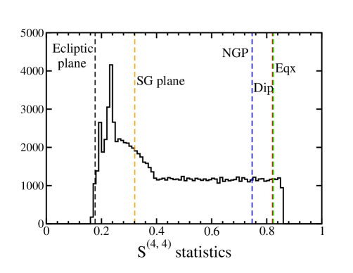
Figure 5: Histogram of the $S^{(4,4)}$ statistics applied to the TOH map quadrupole and octopole area vectors and a fixed direction or plane on the sky, where the area vectors have been rotated together in a random direction $10^{5}$ times. Vertical lines show the $S$ statistics of the actual area vectors applied to the ecliptic plane, NGP, supergalactic plane, dipole and equinox directions (Table 4 shows the actual product percentile ranks among the random rotations for all three full-sky maps). This Figure and Table 4 show that, even given the relative location of the quadrupole-octopole area vectors (i.e. their mutual alignment), the ecliptic plane, dipole and equinox alignments are unlikely at the $\ga 95\%$ C.L. while the NGP and supergalactic plane alignments are not.

Table 4: Percentile ranks of the quadrupole-octopole area vector dot-products with specific directions, among the $10^{5}$ such products where the area vectors have been rotated together in a random direction. We show dot-products for the TOH, LILC and ILC area vectors, and the NEP, NGP, NSGP, dipole and equinox directions. This Table shows that, even given the relative location of the quadrupole-octopole area vectors (i.e. their mutual alignment), the ecliptic plane, dipole and equinox alignments are unlikely at the $\ga 95\%$ C.L. while the NGP and supergalactic ones are not.

Test	TOH DQ-corr	LILC DQ-corr	ILC DQ-corr
ecliptic plane	1.0	0.2	1.7
NGP	87	88	90
SG plane	34	33	25
dipole	95.6	93.8	94.5
equinox	96.1	94.4	96.4

5.5 Single multipole alignment test for $\ell\leq 50$

So far we have devoted attention to alignments of the area vectors defined by the quadrupole and octopole. We would now like to investigate alignment in higher multipoles. To simplify the analysis, we consider a single multipole $\ell$ at a time. We then ask whether the multipole in question is unusually planar. Note however that this test is by no means exhaustive in finding unusual correlations — for example, we are not considering pairs of multipoles, as we did for the quadrupole and octopole. In fact, the octopole, when considered alone, is not unusually planar as first shown by Tegmark et al. (2003) and further illustrated using our tests below. Nevertheless, considering the more complicated tests applied to higher multipoles is not efficient at this time without a specific suspected theory or model in mind. Moreover, we are curious to investigate whether the “bites” observed on the angular power spectrum at a handful of multipoles (Hinshaw et al., 2003a) are somehow correlated to the multipole vector alignments in those multipoles. Therefore, we proceed with testing the single multipole alignment of area vectors.

For a fixed multipole $\ell$ we have $N_{\ell}=\ell(\ell-1)/2$ area (headless) vectors $\mn@boldsymbol{w}_{i}$. We would like to find the plane that is defined by these vectors. We define the plane as the one whose normal, $\hat{\mn@boldsymbol{n}}$, has the largest dot product with the sum of the area vectors. Since $\mn@boldsymbol{w}_{i}\cdot\hat{\mn@boldsymbol{n}}$ is defined only up to a sign, $\mn@boldsymbol{w}_{i}$ is headless, we take the absolute value of each dot product. Therefore, we need to find $\hat{\mn@boldsymbol{n}}$ that maximizes

$$\mathcal{S}\equiv\frac{1}{N_{\ell}}\sum_{i=1}^{N_{\ell}}\left|\mn@boldsymbol{w}_{i}\cdot\hat{\mn@boldsymbol{n}}\right|.$$ (44)

An exact procedure to find the best aligned direction is non-trivial due to the presence of the absolute value. Instead of writing an absolute value we replace $\mn@boldsymbol{w}_{i}$ by $s_{i}\mn@boldsymbol{w}_{i}$, where $s_{i}$ is $\pm 1$, such that there are only positive terms in the sum. The problem is that we cannot know the signs before we know the best aligned directions and thus we have to try out all the possibilities. There are $N_{\ell}$ area vectors, and thus there are $2^{N_{\ell}}$ possible choices for the set $\{s_{i}\}$. As is easily seen, for large $\ell$ this becomes computationally more expensive than a numerical search for the best aligned direction. For any fixed set of signs $\{s_{i}\}$, the best aligned direction $\hat{\mn@boldsymbol{n}}$ expressed in spherical coordinates, $(\theta,\phi)$, is given by

$$\tan\phi = \left.\left(\sum s_{i}w_{i,y}\right)\right/\left(\sum s_{i}w_{i,x}\right)$$ (45)

$$\tan\theta = \left.\left[\sum s_{i}\left(w_{i,x}\cos\phi+w_{i,y}\sin\phi\right)\right]\right/\left(\sum s_{i}w_{i,z}\right),$$

where $w_{i,x}$ denotes the $x$ component of $\mn@boldsymbol{w}_{i}$, etc.

In practice, we used an iterative solution to the problem: pick some trial direction $\hat{\mn@boldsymbol{n}}$ so that we can immediately compute $\mathcal{S}$. Repeat many times for $\hat{\mn@boldsymbol{n}}$ randomly chosen on a unit sphere, and simply find one that has maximal $\mathcal{S}$. We find that the search converges after a few thousand trials for the direction $\hat{\mn@boldsymbol{n}}$.

We compute $\mathcal{S}_{\rm WMAP}$ for any given multipole $\ell$ in the TOH map, and then compare it to the value of $\mathcal{S}_{\rm MC}^{(i)}$, at that multipole, computed in a large number of Monte Carlo realizations of a Gaussian random, statistically isotropic sky with WMAP’s pixel noise added. We then rank-order $\mathcal{S}_{\rm WMAP}$ among the $\mathcal{S}_{MC}^{(i)}$. A low rank indicates that the WMAP areas are roughly aligned, or equivalently, that the multipole vectors are planar and most of the power lies in the corresponding plane. Conversely, a high rank would imply that the multipole in question is non-planar relative to a Gaussian random, statistically isotropic expectation. We use 10,000 Monte Carlo realizations at $l\leq 20$ and at any $l$ that has a very low or high rank in order to obtain sufficient statistics; at all other $\ell$ we use 1000 realizations.

Table 5: Ranks of the $\mathcal{S}$ statistics, R, given as percentiles. Low ranks indicate multipoles that are planar (i.e. their area vectors are aligned), while high ranks indicate multipoles that are non-planar. The statistic $\mathcal{S}$, defined in Eqn. 44, is applied to the TOH cleaned map and compared with Gaussian random, statistically isotropic skies to obtain the ranks. We used 10,000 realizations of such skies for $\ell\leq 20$ and for $\ell=44$, and 1000 realizations for all other multipoles. Values within 5 percentiles of 0 or 100 are shown in bold.

Single-$\ell$ Ranks of the $\mathcal{S}$ Statistic (%)
$\ell$	R	$\ell$	R	$\ell$	R	$\ell$	R	$\ell$	R
2+3	0.35	11	42	21	32	31	33	41	26
2	—	12	19	22	48	32	46	42	3
3	7	13	3	23	20	33	65	43	86
4	75	14	5	24	15	34	11	44	99.7
5	99.7	15	62	25	48	35	13	45	35
6	4	16	4	26	46	36	96	46	31
7	45	17	3	27	96	37	89	47	49
8	77	18	18	28	80	38	47	48	27
9	95	19	19	29	58	39	86	49	91
10	65	20	29	30	4	40	12	50	19

Table 5 shows the ranks of the $\mathcal{S}$ statistic for $3\leq\ell\leq 50$, given as percentages. For example, 25% would indicate that 25% of Monte Carlo maps are more planar and 75% are less planar at that $\ell$. Note that, while the octopole alone is planar only at the 92% C.L., the quadrupole and octopole together are planar at 99.65% C.L. The planarity of the quadrupole and octopole is therefore very significant, in agreement with other tests (see e.g. $A_{i}$ and $D_{i}$ in Table 3). The $\ell=5$, in contrast, is non-planar and only 0.3% of Monte Carlo realizations exhibited lower planarity. What has been called the “sphericity” of $\ell=5$ was first pointed out by Eriksen et al. (2004a); their test found it unusual at the 5-10% level.

Visual inspection of table 5 suggests that there is an excess of both high and low values. Simple attempts to quantify this do indeed find such anomalies at between $95$% C.L. and $99$% C.L. We might therefore conclude that the alignment test as defined in Eqn. (44) gives strong hints of something unusual at $4\leq\ell\leq 50$ in the TOH cleaned map, but without further evidence, the case is not sufficiently strong to stand on its own for any bold claims. Moreover, we find that at $\ell\geq 8$, the values of the $\mathcal{S}$ statistic differ substantially among the TOH, ILC and LILC maps.

Apart from looking at the $\mathcal{S}$ statistics, we also inspected the best aligned directions $\hat{\mn@boldsymbol{n}}$ (the direction that maximize $\mathcal{S}$). We would expect that only the best aligned directions of planar multipoles have a well defined meaning. For $\ell<8$ only $\ell=6$ is singled out by our statistics. We find the corresponding vector at $(l,b)=(152\aas@@fstack{\circ}4,50\aas@@fstack{\circ}3)$, which is $46\aas@@fstack{\circ}2$ from the ecliptic pole. Among the higher best aligned directions, $\ell=21$ and $\ell=44$ are within $2\aas@@fstack{\circ}6$ and $9\aas@@fstack{\circ}0$, respectively, of the dipole. All other vectors are more than $10\degr$ from any physical direction studied in this work.

In addition to the $\mathcal{S}$ statistic described above, we also applied Bingham’s statistic test of isotropy (Fisher et al., 1993; Morgan et al., 2005). Let us assume we have $N$ unit vectors with components $(x_{i},y_{i},z_{i})$ $(i=1,\ldots,N)$ and that we want to check whether they are distributed isotropically. We construct the orientation matrix

$$\mathsf{T}=\frac{1}{N}\sum^{N}_{i=1}\left(\begin{array}[]{ccc}x_{i}x_{i}&x_{i}y_{i}&x_{i}z_{i}\\ y_{i}x_{i}&y_{i}y_{i}&y_{i}z_{i}\\ z_{i}x_{i}&z_{i}y_{i}&z_{i}z_{i}\end{array}\right)\,,$$ (46)

which is real and symmetric with unit trace, so that that the sum of its eigenvalues $e_{k}$ ($k=1,2,3$) is unity. For an isotropic distribution all three eigenvalues should be equal to $1/3$ to within statistical fluctuations. Bingham’s modified statistic ${\cal B}^{\star}$ (Bingham, 1974) is defined as

$${\cal B}^{\star} = {\cal B}\left(1-\frac{1}{N}\left[\frac{47}{84}+\frac{13}{147}{\cal B}+\frac{5}{5292}{\cal B}^{2}\right]\right)\,,{\,\,\,\,\rm where}$$

$${\cal B} = \frac{15N}{2}\sum^{3}_{k=1}\left(e_{k}-\frac{1}{3}\right)^{2}.$$ (47)

For isotropically distributed vectors and $N\gg 1$, ${\cal B}^{\star}$ is distributed as $\chi^{2}_{5}$. Here we compare WMAP’s value of ${\cal B}^{\star}$ for a given multipole to Monte Carlo simulations directly, and therefore do not require assuming $N\gg 1$.

Bingham’s statistic results for $2\leq\ell\leq 50$ are broadly consistent with those for the $\mathcal{S}$ statistic shown in Table 5 (and hence we do not show them separately). We find that $\ell=5$ is non-planar at the $99.8\%$ C.L. but, apart from that, other multipoles are neither planar nor non-planar at a level not expected from such a statistical sample. Finally, note that Bingham’s statistic, being general and coordinate independent, does not use all information and is typically not as strong as the coordinate dependent tests.

5.6 Higher multipole angular momentum vectors

The angular momentum dispersion (19) can be maximized for all multipoles and thus serve as a statistic. That is we can find the axis $\hat{\mn@boldsymbol{n}}_{\ell}$ around which $(\Delta L)_{\ell}^{2}$ is maximized. The spherical harmonics provide an irreducible representation of the rotation group in three dimensions and transform as $\mn@boldsymbol{Y}_{\ell}^{\prime}=\mn@boldsymbol{Y}_{\ell}^{T}\mathsf{D}^{(\ell)}$ where $\mn@boldsymbol{Y}_{\ell}$ is a vector of the $\ell$-th multipole spherical harmonics ($2\ell+1$ components) and $\mathsf{D}^{(\ell)}$ is a rotation of this multipole. Since a scalar function (such as the temperature) is invariant under rotations the $a_{\ell m}$ must transform as $\mn@boldsymbol{a}_{\ell}^{\prime}=\mathsf{D}^{\dagger}\mn@boldsymbol{a}_{\ell}$ under rotations. The rotations can be parametrized in terms of the Euler angles $\alpha$, $\beta$, $\gamma$ in the $zyz$ representation as

$$\mathsf{D}(\alpha\,\beta\,\gamma)=\exp\left(\frac{i\alpha}{\hbar}L_{z}\right)\exp\left(\frac{i\beta}{\hbar}L_{y}\right)\exp\left(\frac{i\gamma}{\hbar}L_{z}\right)$$ (48)

where $L_{y}$ and $L_{z}$ are the $y$ and $z$ components of the angular momentum operator, respectively. The discussion here follows Edmonds (1960). For an alternative representation see appendix A of de Oliveira-Costa et al. (2004).

To perform the maximization it is convenient to use the matrix representation for the rotations

$$D^{(\ell)}_{m^{\prime}m}(\alpha\,\beta\,\gamma)=e^{im^{\prime}\gamma}d^{(\ell)}_{m^{\prime}m}e^{im\alpha},$$ (49)

where

$$d^{(\ell)}_{m^{\prime}m}\!\!\!\! = \!\!\!\!\sum_{k}\frac{(-1)^{\ell-m^{\prime}-k}\sqrt{(\ell+m^{\prime})!(\ell-m^{\prime})!(\ell+m)!(\ell-m)!}}{k!(l-m^{\prime}-k)!(l-m-k)!(m+m^{\prime}+k)!}$$ (50)

$$\quad{}\times\left(\cos\frac{\beta}{2}\right)^{2k+m^{\prime}+m}\left(\sin\frac{\beta}{2}\right)^{2\ell-2k-m^{\prime}-m}.$$

In this representation, the angular momentum dispersion (19) becomes

$$(\Delta L)^{2}_{\ell}\!\!\!\! = \!\!\!\!\sum_{m^{\prime},m^{\prime\prime}}a_{\ell m^{\prime}}^{*}a_{\ell m^{\prime\prime}}e^{i(m^{\prime}-m^{\prime\prime})\gamma}\sum_{m}m^{2}d^{(\ell)}_{m^{\prime}m}(\beta)d^{(\ell)}_{m^{\prime\prime}m}(\beta)$$ (51)

$$\equiv \sum_{m^{\prime},m^{\prime\prime}}H^{(\ell)}_{m^{\prime}m^{\prime\prime}}(\gamma)G^{(\ell)}_{m^{\prime\prime}m^{\prime}}(\beta)$$

$$= \mathop{\rm Tr}\nolimits\left(\mathsf{H}^{(\ell)}(\gamma)\mathsf{G}^{(\ell)}(\beta)\right).$$

Notice that this expression separates into a term that depends only on $\gamma$ and the $a_{\ell m}$, $\mathsf{H}^{(\ell)}(\gamma)$, and a term that only depends on $\beta$, $\mathsf{G}^{(\ell)}(\beta)$. To extremize this function we take derivatives of $(\Delta L)^{2}_{\ell}$ with respect to $\beta$ and $\gamma$ which also separates. It is easy to show that

$$\partial_{\gamma}H^{(\ell)}_{m^{\prime}m^{\prime\prime}}(\gamma)=i(m^{\prime}-m^{\prime\prime})H^{(\ell)}_{m^{\prime}m^{\prime\prime}}(\gamma)$$ (52)

and that both $G^{(\ell)}_{m^{\prime\prime}m^{\prime}}(\beta)$ and $\partial_{\beta}G^{(\ell)}_{m^{\prime\prime}m^{\prime}}(\beta)$ can be calculated quickly and efficiently (see Edmonds (1960) for details). These rotation angles are related to standard Galactic coordinates via

$$(l,b)=(\gamma-180\degr,90\degr-\beta).$$ (53)

Finally, we will find it convenient to work with the normalized angular momentum dispersion (the $t$ statistic of de Oliveira-Costa et al. (2004))

$$(\Delta\tilde{L})^{2}_{\ell}\equiv(\Delta L)^{2}_{\ell}\left/\ell^{2}\sum_{m}\left|a_{\ell m}\right|^{2}\right..$$ (54)

The normalized dispersion takes a value between $(\ell+1)/3\ell$ and one.

Table 6: The maximum angular momentum dispersion results for the TOH cleaned map. Shown in the table is the multipole number, $\ell$, the Galactic coordinates of the direction in which the axis around which the angular momentum dispersion is maximized, $(l,b)$, the value of the normalized angular momentum dispersion around this axis, $(\Delta\tilde{L})_{\ell}^{2}$, and the percentage of Monte Carlos that had a maximum angular momentum dispersion larger than the value found from the TOH map. Values within 5 percentiles of 0 and 100 are shown in bold. See the text for details.

$\ell$	$l$		$b$		$(\Delta\tilde{L})_{\ell}^{2}$	MC Larger
$2\mbox{+}3$	$-112$$\aas@@fstack{\circ}$	$7$	$59$$\aas@@fstack{\circ}$	$7$	$0.962$	$\mathbf{\hphantom{0}0.37\%}$
$2$	$105$$\aas@@fstack{\circ}$	$7$	$56$$\aas@@fstack{\circ}$	$6$	$0.993$	—
$3$	$121$$\aas@@fstack{\circ}$	$6$	$62$$\aas@@fstack{\circ}$	$0$	$0.942$	$11.24\%$
$4$	$-106$$\aas@@fstack{\circ}$	$0$	$36$$\aas@@fstack{\circ}$	$3$	$0.637$	$75.93\%$
$5$	$-170$$\aas@@fstack{\circ}$	$0$	$24$$\aas@@fstack{\circ}$	$0$	$0.484$	$\mathbf{99.44\%}$
$6$	$-160$$\aas@@fstack{\circ}$	$5$	$44$$\aas@@fstack{\circ}$	$1$	$0.817$	$\mathbf{\hphantom{0}3.00\%}$
$7$	$-119$$\aas@@fstack{\circ}$	$7$	$54$$\aas@@fstack{\circ}$	$8$	$0.585$	$58.13\%$
$8$	$149$$\aas@@fstack{\circ}$	$7$	$20$$\aas@@fstack{\circ}$	$1$	$0.546$	$62.28\%$
$9$	$162$$\aas@@fstack{\circ}$	$1$	$77$$\aas@@fstack{\circ}$	$9$	$0.504$	$80.69\%$
$10$	$153$$\aas@@fstack{\circ}$	$8$	$11$$\aas@@fstack{\circ}$	$1$	$0.511$	$70.17\%$
$11$	$-76$$\aas@@fstack{\circ}$	$9$	$12$$\aas@@fstack{\circ}$	$2$	$0.540$	$45.15\%$
$12$	$46$$\aas@@fstack{\circ}$	$3$	$37$$\aas@@fstack{\circ}$	$2$	$0.565$	$28.75\%$
$13$	$-71$$\aas@@fstack{\circ}$	$7$	$41$$\aas@@fstack{\circ}$	$7$	$0.651$	$\mathbf{\hphantom{0}2.73\%}$
$14$	$59$$\aas@@fstack{\circ}$	$3$	$9$$\aas@@fstack{\circ}$	$3$	$0.636$	$\mathbf{\hphantom{0}2.60\%}$
$15$	$-81$$\aas@@fstack{\circ}$	$3$	$31$$\aas@@fstack{\circ}$	$1$	$0.503$	$49.27\%$
$16$	$137$$\aas@@fstack{\circ}$	$9$	$78$$\aas@@fstack{\circ}$	$7$	$0.632$	$\mathbf{\hphantom{0}1.82\%}$
$17$	$-163$$\aas@@fstack{\circ}$	$5$	$30$$\aas@@fstack{\circ}$	$2$	$0.593$	$\mathbf{\hphantom{0}4.70\%}$
$18$	$152$$\aas@@fstack{\circ}$	$8$	$19$$\aas@@fstack{\circ}$	$0$	$0.540$	$14.85\%$
$19$	$-121$$\aas@@fstack{\circ}$	$2$	$60$$\aas@@fstack{\circ}$	$3$	$0.530$	$16.20\%$
$20$	$124$$\aas@@fstack{\circ}$	$2$	$20$$\aas@@fstack{\circ}$	$9$	$0.500$	$28.78\%$

We have maximized the normalized angular momentum dispersion for $\ell=2$ to $20$ for the TOH cleaned map. The ILC and LILC maps give similar results. The results are shown in table 6. For each multipole we provide the direction in Galactic coordinates, $(l,b)$, for the axis around with the angular momentum dispersion is maximized and the value of the maximum angular momentum dispersion. We have also performed 10,000 Monte Carlo simulations of Gaussian random, statistically isotropic skies and found the maximum angular momentum dispersion for each one of them. The final column in the table gives the percentage of MC skies that had an angular momentum dispersion larger than that for the WMAP data. We have also done the same procedure for a joint fit to the quadrupole and octopole ($\ell=2\mbox{+}3$). That is, we find the single axis that maximizes both multipoles.

We find that the octopole is planar, but only at 89% C.L. The strong correlation between the quadrupole and octopole is seen by the fact that less than $0.4\%$ of all Gaussian random, statistically isotropic skies have the quadrupole and octopole this well aligned. We again confirm the “sphericity” of $\ell=5$ first pointed out by Eriksen et al. (2004a). We find the angular momentum dispersion to be very low — all but $0.56\%$ of the MC skies have a value larger than the WMAP data. They have also suggested that $\ell=6$ is planar; by this test it is somewhat planar with only $3\%$ of MC skies being more planar than the data. We find a total of $5$ multipoles that are somewhat planar (less than $5\%$ of MC skies having a larger angular momentum dispersion), those being $\ell=6$, $13$, $14$, $16$, and $17$. We only find the $\ell=5$ multipole to be particularly non-planar.

Setting aside the $\ell=2+3$ result, we see that $6$ of the $18$ angular momentum dispersions are in either the top or bottom 5 percentile. The probability of having $6$ or more of the $18$ so anomalously high or low is $0.6$%. We also see that of these $6$, all but $\ell=5$ are in the top 5 percentile. The probability of having $5$ or more of the $18$ so anomalously high is $0.15$%.

Inspecting the directions of maximum angular momentum dispersion we find that only the $\ell=4$ direction is close to one of the physical directions under consideration: its distance to the ecliptic pole is $10\aas@@fstack{\circ}3$. Note that this confirms the qualitative impression from looking at the $\ell=4$ map (see Schwarz et al. (2004)) that this mode has its minima and maxima aligned with the ecliptic plane. It is also interesting to note that the directions given in table 6, especially for the planar multipoles, are consistent with the ones found as the best aligned directions.

These results are another suggestion that the higher $\ell$ multipoles are not statistically isotropic. Reassuringly, comparison of Tables 5 and 6 shows the same $5$ multipoles which had a high angular momentum dispersion also exhibited comparably low ranks of the $\mathcal{S}$ statistic, while $\ell=5$ showed a high rank of $\mathcal{S}$. This difference in range of $\ell$ in Secs. 5.6 and 5.5 was purely a result of computational limitations.

5.7 “Shape” statistic

The angular momentum dispersion searches for planarity through a weighted average that favors modes with $m=\ell$. Land & Magueijo (2005a) have suggested the use of the “shape” statistic which finds the preferred axis and the preferred $m$ for each multipole. The statistic is defined as

$$r_{\ell}=\max_{m,\hat{\mn@boldsymbol{n}}}r^{(\ell)}_{m}$$ (55)

where

$$r^{(\ell)}_{m}\equiv\left(2-\delta_{m,0}\right)\left|a_{\ell m}\right|^{2}\left/\sum_{m}\left|a_{\ell m}\right|^{2}\right..$$ (56)

and $\hat{\mn@boldsymbol{n}}$ is the $z$-axis of the coordinate system in which the $a_{\ell m}$ are computed. Note that the angular momentum dispersion is a weighted sum of these terms,

$$(\Delta L)^{2}_{\ell}=\frac{1}{\ell^{2}}\sum_{m=0}^{\ell}m^{2}r^{(\ell)}_{m}.$$ (57)

The maximization of the shape statistic (55) follows the same formalism as for the angular momentum dispersion and will not be discussed further (see Sec. 5.6). We have performed this maximization and confirm the results of Land & Magueijo (2005a). In particular, we find that the surface defined by $r_{\ell}$ is complicated with many local maxima. The results are quite sensitive to the data and are not consistent among the three full-sky maps made from the WMAP data (see Fig. 2 of Land & Magueijo (2005a)). Unfortunately this sensitivity is not understood in terms of features of the data. That is, the variability in the results cannot be understood in terms of features such as non-Gaussianity or a violation of statistical isotropy. The sensitivity of the shape statistic is related to the difficulty in uniquely defining the Land-Magueijo vectors (Land & Magueijo 2005e, also see Sec. 3.5). For these reasons, the shape statistic does not serve as a robust statistic for separating nor understanding Gaussianity versus statistical isotropy.

6 Foregrounds

So far, we have taken into account the effects of noise in the full-sky cleaned maps by including the WMAP pixel noise into our Monte Carlos. We now explore the effect of the foregrounds on the quadrupole-octopole anomaly.

While it has repeatedly been emphasized that there might be residual foreground contamination left in the cleaned maps, it seems that such a contamination should lead to Galactic and not ecliptic correlations. Here we explicitly show this with a quantitative analysis. We slowly add the measured WMAP foreground contaminations to WMAP full-sky maps and monitor how the directions defined by the quadrupole and octopole change.

Figure 6: Trajectories of the multipole vectors and their normals as increasing amounts of the foreground is added to or subtracted from the microwave background map. We have use the synchrotron V-band foreground and the TOH cleaned map; the coefficient $c$ shows the rms contribution of the foreground to the microwave background (see Eqns. 58 and 59). The solid diamond symbols show the zero-foreground locations of the multipole vectors while the solid stars refer to their pure-foreground locations. Similarly, the open diamond and star symbols refer to the beginning and end points of the normal vectors. On each trajectory we label a few values of the coefficient $c$. The top panel shows $\ell=2$ (two vector and one normal) and the bottom panel shows $\ell=3$ (three vectors and three normals). Not all trajectories end on plotted symbols. For these trajectories they end on the multipole vector (or normal) that is the negative of the plotted vector at the start of the trajectory. Note that, in the large-foreground limit, the quadrupole vectors move near the $z$-axis and the normal into the Galactic plane, while for the octopole all three normals become close to the Galactic disk at $90^{\circ}$ from the Galactic center. Therefore, as expected Galactic foregrounds lead to Galactic, and not ecliptic, correlations of the quadrupole and octopole.

Let $T_{\rm CMB}(\hat{\mn@boldsymbol{n}})$ be the cleaned-map microwave background temperature in some direction, and $T_{\rm FOR}(\hat{\mn@boldsymbol{n}})$ the temperature from one of the three basic foreground maps (thermal dust, free-free emission or synchrotron emission) provided by the WMAP team. We form the total contaminated map as

$$T_{\rm tot}(\hat{\mn@boldsymbol{n}})=T_{\rm CMB}(\hat{\mn@boldsymbol{n}})+c\,T_{\rm FOR}(\hat{\mn@boldsymbol{n}})\sqrt{\mathop{\rm Var}\nolimits(T_{\rm CMB})\over\mathop{\rm Var}\nolimits(T_{\rm FOR})}.$$ (58)

where $c$ is the foreground fraction. Note that the second term has been normalized so that

$$\mathop{\rm Var}\nolimits(T_{\rm tot}) = \mathop{\rm Var}\nolimits(T_{\rm CMB})+c^{2}\,\mathop{\rm Var}\nolimits(T_{\rm FOR}){\mathop{\rm Var}\nolimits(T_{\rm CMB})\over\mathop{\rm Var}\nolimits(T_{\rm FOR})}$$ (59)

$$= \mathop{\rm Var}\nolimits(T_{\rm CMB})(1+c^{2})$$

so that the rms contribution to the total rms temperature from the added foreground is a factor, $c$, relative to the contribution of the cleaned microwave background map. (For reference, the constant $\sqrt{\mathop{\rm Var}\nolimits(T_{\rm CMB})/\mathop{\rm Var}\nolimits(T_{\rm FOR})}$ is of order unity in all cases we consider.) In Copi et al. (2004), we have performed tests with $c\leq 0.2$ and found no significant changes to the results in that paper. Note that the contribution in power of known foregrounds to the microwave background, after removing the foregrounds, is estimated to be less than a percent in the V and W bands (Bennett et al., 2003a). However this estimate is for the multipole range $2\leq\ell\leq 100$ while the foreground contamination is most significant at low multipoles (see Fig. 10 in Bennett et al. 2003a). Therefore it is reasonable to assume that the contribution of residual foregrounds at large angular scales is less than about 10% in power, or $c\la 0.3$.

We have added increasing amounts of foreground, corresponding to $c$ taking values from zero (no foreground) to $\pm$ 1000 (essentially pure foreground) and recomputed the multipole vectors and their normals. Fig. 6 shows the trajectories of the multipole vectors and their normals as increasing amount of the foreground (V-band synchrotron map produced by WMAP) is added to the microwave background map. The solid diamond symbols show the zero-foreground locations of the multipole vectors while the solid stars refer to their pure-foreground locations. Similarly, the empty diamond and star symbols refer to the zero- and pure-foreground normal vectors. On each trajectory we label a few positive and negative values of the coefficient $c$. The top panel of Fig. 6 shows $\ell=2$ (two vector and one normal) and the bottom panel shows $\ell=3$ (three vectors and three normals).

In the pure-foreground limit, the quadrupole vectors move near the $z$-axis and their normal into the Galactic plane as is expected for an almost pure $Y_{20}$ mode (see the discussion in Sec. 2.2). In the same limit, two of the octopole multipole vectors move close to the Galactic poles and one close to the Galactic center. Consequently, all three normals become close to the Galactic disk at $90^{\circ}$ from the Galactic center. This is indeed the signature of the expected $\mathrm{Re}(Y_{31})$ domination in the foreground octopole. Therefore, both the vectors and their normals clearly migrate from locations correlated with the ecliptic and other directions discussed in Schwarz et al. (2004) and in this paper to locations specified by the Galactic foreground emission. Further, note that appreciable admixture of the foreground ($|c|\ga 0.1$ for the quadrupole and $|c|\ga 0.3$ for the octopole) is necessary for this migration to become apparent by eye. This confirms the argument in Sec. 2.2 that the quadrupole foreground is the most critical one.

The reader might notice that two of the octopole multipole vectors are within $10\degr$ of the Galactic plane, or, equivalently, one of the octopole normals is about $10\degr$ from the Galactic poles. One might ask if that could be a sign of residual Galactic contamination of the cleaned full-sky maps. However, as seen in figure 5 and table 4, given the observed pattern of quadrupole and octopole area vectors, the alignment of these area vectors with the NGP is significant at $<90$% C.L. (compared to a 99% C.L. correlation with the ecliptic plane). Moreveor, since a correlation of the normal with the Galactic plane would have been even at least as noteworthy, this 90% C.L. figure should be reduced to 80%.

We also observe that when adding foreground, one of the two multipole vectors close to the Galactic plane moves far away from that plane. The other multipole vector close to the Galactic centre does not move very far (about $10\degr$). But, a $10\degr$ alignment of one of the cleaned-map multipole vectors with one of the foreground multipole vectors is not statistically significant by any statistical test applied in this work. Even less so when we consider that we would remarked as well on a similar alignment of a cleaned-map area vector with a foreground area vector.

Finally, we do not expect more than one foreground multipole vector to lie near the Galactic plane since the dominant fairground mode of the octopole is indeed $\mathrm{Re}(Y_{31})$. The second biggest foreground mode is $\mathrm{Re}(Y_{33})$, which has its three multipole vectors in the Galactic plane at $l=30\degr$, $90\degr$ and $150\degr$. But, the cleaned full-sky map does not resemble that pattern either. We are not able to identify a Galactic contamination of the cleaned full-sky maps and thus see no evidence to question more significant ecliptic correlations found in the previous sections.

We have checked that the results are qualitatively unchanged if we use the W-band synchrotron map, or the V-band free-free and dust foreground maps instead of the V-band synchrotron map. We have done some further testing, recomputing the $S$ statistics applied to different alignments but now with the foreground incrementally added to both the microwave background and Monte Carlo maps. We found that the results are consistent with those inferred from Fig. 6 and indicate that large admixture of the known Galactic foreground would not cause the alignments found in Schwarz et al. (2004).

Results of this investigation are therefore in agreement with the intuitive expectation: Galactic foregrounds lead to Galactic, and neither ecliptic nor dipole, correlations of the quadrupole and octopole. In fact, it is difficult to see how any known foreground that has most of its power in the Galactic plane can lead to the solar system correlations that we find.

7 Effects of cut skies

As mentioned in Copi et al. (2004), Galaxy cuts of a few degrees or larger introduce significant uncertainties to the reconstructed full-sky multipole vectors. This is precisely why we used the cleaned full-sky maps — sky cuts of 20 degrees or so would simply lead to large uncertainties in our statistical tests. Nevertheless, we would like to look at the issue of sky cuts in more detail; in particular, we would like to explore how correlation significance varies as we introduce a sky cut.

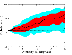
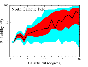
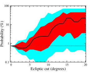
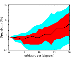
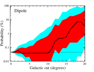
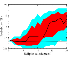
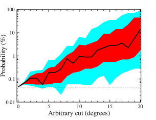
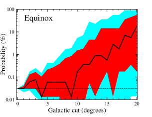
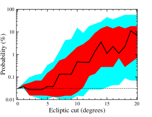
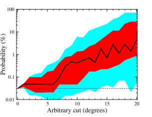
Figure 7: Quadrupole-octopole probabilities for the TOH DQ-corrected map for an increasingly larger isolatitude cut of $\pm$(degrees shown), performed symmetrically around the Galactic plane (left column), ecliptic plane (central column) or an arbitrarily chosen plane (right column). We consider the $S$ statistic probabilities applied to the ecliptic plane, north Galactic pole, dipole and the equinoxes (first to fourth row respectively). The solid line is the mean value, while the dark and light regions represent 68% C.L. and 95% C.L. regions, respectively, from 1000 realizations of reconstructed $a_{\ell m}$ coefficients that take into account the noise in the reconstruction process. The dashed line denotes the probability obtained from the full-sky map, corresponding to the case of zero cut.

We are interested in finding the full-sky (true) $a_{\ell m}$ which are derived from the full-sky temperature distribution and denoted by $a_{\ell m}^{t}$. In general, we cannot view the full sky as the Galaxy obscures our field of view and must be cut out. There are well know techniques for relating the cut sky decomposition, $a_{\ell m}^{c}$, to the true sky decomposition (Wandelt et al., 2001; Mortlock et al., 2002). We briefly discuss the key facts here. The decompositions are related by

$$a_{\ell m}^{c}=\sum_{\ell^{\prime}m^{\prime}}W_{\ell\ell^{\prime},mm^{\prime}}a_{\ell^{\prime}m^{\prime}}^{t}$$ (60)

where

$$W_{\ell\ell^{\prime},mm^{\prime}}\equiv\int_{S_{\rm cut}}Y_{\ell^{\prime}m^{\prime}}^{*}(\Omega)Y_{\ell m}(\Omega)\mathrm{d}\Omega$$ (61)

and $S_{\rm cut}$ is the cut sphere. There are fast, stable recursion relations for calculating these $W_{\ell\ell^{\prime},mm^{\prime}}$ (Wandelt et al., 2001; Mortlock et al., 2002). In this work, we restrict ourselves to longitudinal cuts symmetric across the Galactic ($xy$) plane. In this case, $m=m^{\prime}$ and $\mathsf{W}$ is a symmetric matrix. For notational convenience we will drop the $m$ index and keep in mind that the subsequent equations hold independently for each $m$. Thus we write

$$a_{\ell}^{c}=\sum_{\ell^{\prime}}W_{\ell\ell^{\prime}}a_{\ell^{\prime}}^{t}.$$ (62)

Since information is lost in the cut, $\mathsf{W}$ is not an invertible matrix. We can, however, replace $\mathsf{W}$ with an invertible matrix $\mathsf{\tilde{W}}$ constructed from $\mathsf{W}$ by removing the rows and columns with small eigenvalues. That is, $\mathsf{\tilde{W}}\equiv\mathsf{\tilde{V}}\mathsf{\tilde{\lambda}}\mathsf{\tilde{V}}^{T}$ where $\mathsf{\tilde{\lambda}}$ is the diagonal matrix of eigenvalues such that $\tilde{\lambda}_{j}=\lambda_{j}$ if $\lambda_{j}>\lambda_{\rm threshold}$ and $\tilde{\lambda}_{j}=\tilde{\lambda}_{j}^{-1}=0$ otherwise. A threshold of $\lambda_{\rm threshold}<0.1$ is typically sufficient and is used in this analysis. An estimate, $\tilde{a}_{\ell}^{t}$ for the true decomposition is

$$\tilde{a}_{\ell}^{t}=\sum_{\ell^{\prime}}\tilde{W}_{\ell\ell^{\prime}}^{-1}a_{\ell^{\prime}}^{c}.$$ (63)

We can prevent leakage of power from non-cosmological monopole and dipole modes by projecting out these modes using a partial Householder transformation (see Appendix C of Mortlock et al. 2002 for details).

There is an error in this approximation which is evident from the fact that

$$\tilde{\mn@boldsymbol{a}}^{t}=\mathsf{\tilde{W}}^{-1}\mn@boldsymbol{a}^{c}=\mathsf{\tilde{W}}^{-1}\mathsf{W}\mn@boldsymbol{a}^{t}$$ (64)

and $\mathsf{\tilde{W}}^{-1}\mathsf{W}\neq\mathsf{I}$ due to the loss of information in the cut. Our error in the approximation is found to be

$$\left\langle\left|\mn@boldsymbol{a}^{t}-\tilde{\mn@boldsymbol{a}}^{t}\right|^{2}\right\rangle = \left\langle\left(\mn@boldsymbol{a}^{t}-\tilde{\mn@boldsymbol{a}}^{t}\right)^{*}\left(\mn@boldsymbol{a}^{t}-\tilde{\mn@boldsymbol{a}}^{t}\right)^{T}\right\rangle$$

$$= \left(\mathsf{I}-\mathsf{\tilde{W}}^{-1}\mathsf{W}\right)\left\langle(\mn@boldsymbol{a}^{t})^{*}(\mn@boldsymbol{a}^{t})^{T}\right\rangle\left(\mathsf{I}-\mathsf{\tilde{W}}^{-1}\mathsf{W}\right)^{T}.$$

Here $\langle(a^{t}_{\ell})^{*}a^{t}_{\ell}\rangle={\cal C}_{\ell}$ and this error can be readily calculated.

Fig. 7 shows the quadrupole-octopole correlation probabilities with the sky cut between zero and $\pm$20 degrees performed along the Galactic plane (left column), ecliptic plane (central column) or an arbitrarily chosen plane (right column). We consider the $S$ statistic probabilities applied to the ecliptic plane, north Galactic pole, dipole and the equinoxes (first to fourth row respectively). The solid line is the mean value, while the dark and light regions represent 68% C.L. and 95% C.L. regions, respectively, from 1000 realizations of reconstructed $a_{\ell m}$ coefficients that take into account the noise in the reconstruction process. While the increasing cut clearly increases error in the vector reconstruction and therefore uncertainty in the final probability, it is clear that in essentially all cases the probabilities remain consistent with the full-sky values at 95% C.L., and in most cases at the 68% C.L. for cuts up to 10 degrees.

This figure clearly shows that sky cuts of a few degrees or larger introduce significant uncertainty in the extracted multipole vectors and their normals, leading to increased error in all alignment tests. Nevertheless, the cut-sky alignments are consistent with their full-sky values even for relatively large cuts. Note that the shift of the mean value of the alignments (black curves in the panels of Fig. 7) to less significant values, as the cut is increased, is entirely expected: an unlikely event, in the presence of noise in the data, becomes less unlikely because any perturbation will shift the multipole and area vectors away from their aligned locations. While the results of this exercise are in good agreement with those found by Slosar & Seljak (2004) and Bielewicz et al. (2005), unlike these authors, we emphasize that the cut sky is always expected to lead to shift in the alignment values and to increased errors (see again Fig. 7).

8 Comparisons with COBE

Since the alignments we are studying are on very large scales (i.e. quadrupole and octopole scales), it is natural to ask whether they can be seen in COBE-DMR maps (Bennett et al., 1996). COBE angular resolution is about $7\degr$, which is more than sufficient for this test. However, full-sky maps produced by the COBE team are very noisy (G. Hinshaw, private communication) while, as discussed in Sec. 7, using the cut sky maps produces too much uncertainty in the vectors for Galaxy cuts larger than a few degrees.

Fortunately, Markov chain Monte Carlo (MCMC) Gibbs sampler realizations of the full-sky COBE maps have been produced. Using their Global Estimation Method, Wandelt et al. (2004) generate 10,000 realizations of the COBE sky consistent with DMR measurements and expected foregrounds. Following their own conservative approach, we drop the first 1000 maps which might be affected by the burn-in of the MCMC, and choose every 200th map from the remaining 9000. The resulting 45 maps are essentially uncorrelated and their analysis is computationally undemanding. We then compute the $S$ statistic for each COBE map and rank-order it relative to 100,000 Monte Carlo realizations of the Gaussian random, statistically isotropic sky. The COBE derived values for the statistic $S$ is represented by histograms, while a WMAP full-sky map is represented by a single value. We then ask whether the two are consistent. Note that we have corrected all COBE maps for the DQ using the procedure described in Sec. 2.4.

The results are shown in Fig. 8. The $x$-axis in each panel shows the logarithm of the probability of $S$ (the probability is simply its rank relative to 100,000 Monte Carlo realizations of the Gaussian random, statistically isotropic sky). The vertical lines show values for the TOH, ILC and LILC maps. The histogram shows values for the 45 COBE maps produced using the MCMC Gibbs sampler. Obviously, there is significant variation in the COBE statistics which traces to the fact that the MCMC maps are based on incomplete sky information. Nevertheless, we see that the statistically significant alignments found with WMAP are in most cases consistent to the results from COBE. For example, 11 out of 45 COBE maps show the alignment with the north ecliptic pole that is equally or less likely than that in the WMAP maps, while 4 to 8 COBE maps (depending on which WMAP map is considered) show equal or less likely alignment with the equinoxes. Note too that the alignment with the supergalactic plane differs significantly in the three WMAP maps. Consequently, the comparison of MCMC-derived COBE maps with WMAP cleaned full-sky maps shows that COBE data are consistent with WMAP in regards to all alignments found in Schwarz et al. (2004).

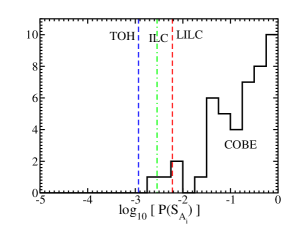
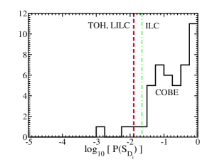
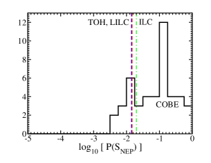
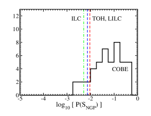
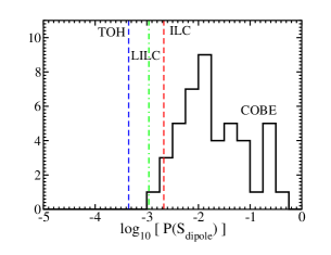
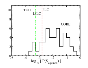
Figure 8: The oriented area statistics from full-sky WMAP maps compared to those from Markov chain Monte Carlo realizations of the COBE full sky based on COBE-DMR cut-sky data. We consider the $S$ statistic applied to the dot-products of quadrupole-octopole area vectors ($A_{i}$) and the normals ($D_{i}$), as well as the sum (i.e. the $S$-statistic) of the four dot-products of the area vectors, one quadrupole and three octopole, with the special directions or planes — the ecliptic plane, NGP, dipole and equinox. The WMAP maps considered for the TOH, ILC and LILC as shown by the vertical lines. The histograms are from a total of 45 MCMC COBE maps from Wandelt et al. (2004) (their maps 1000, 1200, …, 9800) which are sufficiently separated in the chain so as to be essentially uncorrelated.

9 Angular Power spectrum — ecliptic plane versus ecliptic poles

There are at least three points in the binned WMAP angular TT power spectrum that deviate from the predictions of the best fit $\Lambda$CDM model at comparable or greater statistical significance to the power deviation of the quadrupole. These are clearly seen in Fig. 12 of Bennett et al. (2003b) in the bins $\ell=20\mbox{--}24$, $\ell=37\mbox{--}44$ and $\ell=201\mbox{--}220$, which are visibly low, high and low respectively. These deviations are approximately 2, 2.5 and 1.5 times the estimated error in the average $C_{\ell}$ in each of those bins. In each case, this is largely cosmic variance dominated, with only a small fraction of the error being due to statistical error. Nevertheless, it should be appreciated that the statistical significance of these deviations may decline in the second or third year WMAP maps.

Various explanations have been offered for these deviations in the angular power spectrum as arising from fundamental physics (e.g. Gordon & Hu (2004); Enqvist et al. (2005) and references therein). However, it is instructive to examine the angular power spectrum computed separately using data from the ecliptic plane versus data from the ecliptic pole. This is presented in Fig. 7 of Hinshaw et al. (2003b). [Note that this Figure has been replaced in the final, published version of the paper (Hinshaw et al., 2003a) with a cross-band power spectrum that shows some of the same features.] The figure caption instructs the reader to “note that some of the ‘bite’ features that appear in the combined spectrum are not robust to data excision.” Specifically, the three deviations at $\ell\approx 22$, $40$ and $210$ are found only in the ecliptic polar data and not in the ecliptic planar data. This suggests that there are some continuous parameters — the latitude of the planar-polar division, the orientation of the reference plane relative to the ecliptic, etc. — as a function of which the separation is approximately maximized by the WMAP team’s choice of an ecliptic planar-polar division.

A more detailed study is merited after future data releases. In the meantime, the dip at the first peak, while the least significant, has the virtue of being in a region of the angular power spectrum that has previously been probed by multiple experiments — TOCO (Torbet et al., 1999; Miller et al., 1999), Saskatoon (Netterfield et al., 1996), Boomerang (Netterfield et al., 2002; Jones et al., 2005), Maxima (Hanany et al., 2000), and Archeops (Benoit et al., 2003; Tristram et al., 2005). Of these, only Archeops saw evidence of a dip in the power at the first peak, though it was of limited statistical significance. Other experiments, saw no such dip with greater statistical confidence. However, other than WMAP only Archeops covered a significant portion of the north ecliptic hemisphere; the others covered much less sky or the southern-sky. Thus if the dip in the first peak is localized to the northern sky, especially to the region near the north ecliptic pole, all the experiments could be consistent. Notably, Archeops also shows evidence of excess of power at $\ell\simeq 40$.

Figure 7 of Hinshaw et al. (2003b) contains further perplexing anomalies in the low-$\ell$ sky — the angular power spectra extracted from the ecliptic planar and polar regions disagree for $\ell<10$. The differences are much larger than would be expected from statistics alone, these low-$\ell$ $C_{\ell}$’s being very well measured (as can be seen from the error bars in Fig. 8 of the same paper):
1) There is a nearly complete absence of ecliptic polar power in the $\ell=6-7$ bin that is highly reminiscent of the findings in tables 5 and 6 that $\ell=6$ is very “planar.” This suggests further that said planarity is closely aligned with the ecliptic, and that this connection extends to $\ell=7$ as well. This is also reflected by the fact that the best aligned vectors for $\ell=6$ and $\ell=7$ from Sec. 5.5 are $46^{\circ}$ and $23^{\circ}$, respectively, from the ecliptic pole, which already indicates that there is little power in the (ecliptic) polar cap region defined as $\beta>30^{\circ}$ in the WMAP analysis.
2) The aplanarity of $\ell=5$ (and to a lesser extent $\ell=4$), as seen again in tables 5 and 6, may also be reflected in the notably even distribution of power between the plane and poles.
3) There is a dramatic deficit in ecliptic planar power compared to ecliptic polar power at $\ell=2$ and $\ell=3$.

If indeed there is contamination of the microwave background from some source in the ecliptic (north?) polar region that is responsible for the deviations at $\ell\approx 22,40$ and $210$, then it is possible that this contamination is also the source of the low-$\ell$ microwave background in the polar regions. In this case, the maximum cosmic contribution to the CMB at low $\ell$’s would be the lesser of the ecliptic planar and polar values (barring an exceptional cancellation). In particular, the cosmic $C_{2}$ and $C_{3}$ would be bounded by the ecliptic (planar) values. These are dramatically lower than the customary values as extracted from the full sky with a Galactic cut, and considerably less consistent with theoretical expectations than even the current low values.

10 Conclusion

The multipole vector formalism first introduced to the study of the CMB by Copi et al. (2004) has proven to be a useful means of studying the structure of the CMB particularly on large scales. In this work, we have provided an extensive discussion of the multipole vector formalism highlighting the fact that the multipole vectors provide an alternative, complete representation of a scalar function on a sphere (see Sec. 3 for details). In particular, we have pointed out that the algorithm of Copi et al. (2004) converts the standard spherical harmonic decomposition into the multipole vector representation first discussed by Maxwell (18). We have shown how the multipole vector formalism relates to the previously studied maximum angular momentum dispersion (MAMD) directions, Land-Magueijo vectors, and temperature minima/maxima directions. Note that, unlike the multipole vectors, neither the MAMD nor the minima/maxima directions contain the full information of a multipole, and are thus not complete representations of the microwave sky. The Land-Magueijo vectors and scalars are a complete representation, but suffer from a rapid proliferation of arbitrary choices for $\ell>2$.

As noted, the multipole vectors are an excellent way to study alignments and correlations in the microwave sky. We have provided a qualitative description of the striking properties of the quadrupole and octopole in Sec. 4. We note that there are strange properties for the quadrupole and octopole individually as well as jointly. Not all of these unexpected properties are independent of each other and an explanation, whether statistical fluke, residual foreground contamination, or real CMB features, remains to be determined.

By eye the properties of the quadrupole and octopole multipole vectors seen in Figs. 1–3 are striking. To quantify these correlation we have used the $S$ and $T$ statistics for the oriented area and normal vectors (see Sec. 5.2) and applied them to the quadrupole and octopole (see Sec. 5.3). We confirm the alignment of the quadrupole and octopole planes at greater than $99$% C.L. We also confirm that the quadrupole-octopole planes are aligned with the geometry and direction of motion of the solar system. In particular, they are perpendicular to the ecliptic plane at approximately $98$% C.L. and to the dipole and equinox at $>99.8$% C.L. They are also perpendicular to the Galactic poles at $>99$% C.L.

We have shown that the alignment with the ecliptic plane remains at 99% C.L. when the quadrupole-octopole alignment is taken as given (for the TOH-DQ map; similar or stronger results hold for the other maps, see Sec. 5.4). The correlations with the dipole and equinox remain at approximately the 95% C.L. However, the correlations with other directions, such as the Galactic poles, do not persist. This strongly supports the reality of the ecliptic correlation in the data and suggests that the aforementioned alignment with the Galactic poles is accidental.

We further stress that the 99% C.L. correlation of the quadrupole-octopole planes with the ecliptic plane is a lower bound. As is evident from Fig. 3 and discussed in more detail in Sec. 5.4 the ecliptic plane carefully threads its way between the temperature minima and maxima of the $\ell=2+3$ map separating the weak power in the northern ecliptic sky from the strong power in the southern ecliptic sky. This extra feature that is manifest in the multipole vectors is not contained in our statistics of oriented area (nor normal) vectors. Thus the analyses discussed in this work and in the literature which rely solely on dot-products of the oriented area (or normal) vectors are not using all the information available in the multipole vectors. Dot-products of oriented area (and normal) vectors are well suited for identifying and defining planes but do so at the expense of the information of the structure with respect to these planes. (For the quadrupole the area vector contains only three out of four pieces of information, the normal only two. For the octopole the complete information is contained in the three normals, but the dot-product statistic misses several degrees of freedom.) We have estimated that including this extra structure strengthens the 99% C.L. bound on the correlation of the quadrupole-octopole with the ecliptic plane to between $99.93$% C.L. (for the ILC map) and $99.996$% C.L. (for the LILC map).

In this work, we have continued to use cleaned, full-sky maps produced from the first year WMAP data. The concern with using these maps is the potential for residual Galactic foregrounds biasing the results. Though it is difficult to see how Galactic contaminations can lead to ecliptic correlations, we have studied this in two different ways: we have explored the properties of the foreground multipole vectors (in Sec. 6) and we have explored how the multipole vectors and our results change when we perform a symmetric cut across the Galactic (and other) planes (in Sec. 7). As expected a Galactic foreground is dominated by the $Y_{20}$ and $\mathrm{Re}(Y_{31})$ modes. These are very different from the modes that dominate in the full-sky maps. As shown in Fig. 6 this corresponds to the multipole vectors and normals for the full-sky maps being in very different locations than those for the foregrounds. As foreground contamination is slowly added to the full-sky maps we see how the full-sky multipole vectors move to the foreground multipole vectors. We have found that large foreground contaminations ($|c|\approx 0.3$ for the quadrupole, $|c|\approx 1\mbox{--}3$ for the octopole) are required to make the full-sky multipole vectors look like those from the known foreground maps.

An alternative to using foreground maps is to mask out all information in the regions of the sky dominated by foregrounds. This is a more conservative approach but throws away information about the CMB in some regions of the sky. For this reason any results from such a cut sky analysis will be weaker than the corresponding full-sky analysis. In Sec. 7, we considered symmetric cuts across the Galactic (and other) planes to access the effect on the multipole vectors and correlations we have found from the full-sky analyses. As seen in Fig. 7 even small cuts lead to large uncertainties in our results. This is true independent of the plane about which we cut. The correlations we report from the full sky remain consistent in the cut sky analysis but are weakened as expected. This result is consistent with the power equalization reconstruction by Bielewicz et al. (2005) the cut sky analysis of Slosar & Seljak (2004).

As a final comparison of the quadrupole and octopole alignments we calculated the correlations for COBE maps (see Sec. 8). Again the results are consistent with those from the WMAP full-sky maps (as shown in Fig. 8) but do not have the statistical significance.

The lack of power on the largest angular scales first observed by COBE and more recently confirmed by WMAP has motivated much of the study of the low multipole moments, in particular the quadrupole and octopole. However, these are not the only multipole bands where there are peculiar features in the power spectrum. We have extended some of the studies to higher multipoles (Secs. 5.5 and 5.6). Our tests suggest that there may exist peculiarities in these multipole ranges not solely in the power, but also in the structure of the multipoles. These studies, however, are not complete and thus it is not possible to assign statistical significance to them. They do, however, point the way for future work.

To conclude, using the multipole vector decomposition we have shown that the quadrupole and octopole of the microwave background sky are correlated with each other at a level that is excluded from being chance in excess of 99%. This comes about from a preponderance of peculiar correlations and is statistically independent of their observed lack of power. This observation is in bold contradiction to the predictions of pre-existing cosmological model, and argues against an inflationary origin for these fluctuations. In addition, there is strong evidence (again of greater than 99% confidence) that the microwave background at these multipoles is correlated with the geometry and direction of motion of the solar system. The observed signal is most unlikely to be due to residual contamination of the full-sky microwave background maps by known Galactic foregrounds.

These results strongly suggest that either there is additional, unexplained foreground contamination of the microwave background, potentially from a source local to our solar system or its neighborhood, or that there is an unexpected systematic error in the WMAP maps. We remain convinced by the WMAP team’s arguments that there is no unexpected systematic error (Bennett et al. 2003a; see also Finkbeiner 2004). In particular, it is very hard to see how a north-south ecliptic asymmetry, or a quadrupole-octopole plane perpendicular to the ecliptic could be induced in the WMAP instrument or analysis pipeline. COBE, with largely independent error sources, saw compatible correlations. There is also the tantalizing suggestion by Archeops of a deficit in power near the first peak which is localized on the sky to the region of the ecliptic north pole.

The astute reader will note that we have persisted in our failure to offer either a satisfactory possible explanation for an ecliptic-correlated foreground (especially one apparently concentrated in a plane perpendicular to the ecliptic) or a prediction that can be convincingly tested. Both are failings which we intend to remedy in the near future. However, we note that should indeed the low-$\ell$ microwave background prove to be dominated by a new foreground, this would imply that, barring an unexpected foreground alignment, the power in the underlying cosmic contribution at these multipoles is likely to be suppressed below even the currently observed too-low value. It is at least amusing to note that the scale on which the lack of large scale correlations is then manifested is comparable to the horizon scale at the onset of cosmic acceleration. At the least this profound lack of large-angle correlations would further challenge generic inflationary models, maybe even general relativity on the scale of the observable universe will need to be reconsidered.

Whatever the origin of these low-$\ell$ correlations, it is clearly necessary to reconsider any inferences drawn from the low-$\ell$ WMAP data, including the temperature-polarization cross-correlation. For example, our work suggests that the evidence for early reionization of the universe, resting as it does on the low-$\ell$ TE angular power spectrum should be viewed with a healthy dose of skepticism.

On the experimental side, we are eagerly waiting for two new major and largely independent probes of the large-angle microwave background radiation that may shed new light on the anomalies discussed in this paper: polarization measurements by WMAP (though they are expected to be systematics-dominated on large scales), and measurements of temperature and polarization by the Planck experiment.

References

- Bennett et al. (1996) Bennett C. L., et al., 1996, ApJ, 464, L1
- Bennett et al. (2003a) Bennett C. L., et al., 2003a, ApJS, 148, 97
- Bennett et al. (2003b) Bennett C. L., et al., 2003b, ApJS, 148, 1
- Benoit et al. (2003) Benoit A., et al., 2003, A&A, 399, L19
- Bielewicz et al. (2005) Bielewicz P., Eriksen H. K., Banday A. J., Górski K. M., Lilje P. B., 2005, astro-ph/0507186
- Bielewicz et al. (2004) Bielewicz P., Górski K. M., Banday A. J., 2004, MNRAS, 355, 1283
- Bingham (1974) Bingham C., 1974, Ann. Stat., 2, 1201
- Cayon et al. (2005) Cayon L., Jin J., Treaster A., 2005, astro-ph/0507246
- Chiang et al. (2003) Chiang L.-Y., Naselsky P. D., Verkhodanov O. V., Way M. J., 2003, ApJ, 590, L65
- Copi et al. (2004) Copi C. J., Huterer D., Starkman G. D., 2004, Phys. Rev., D70, 043515
- Cruz et al. (2005) Cruz M., Martinez-Gonzalez E., Vielva P., Cayon L., 2005, MNRAS, 356, 29
- de Oliveira-Costa et al. (2004) de Oliveira-Costa A., Tegmark M., Zaldarriaga M., Hamilton A., 2004, Phys. Rev., D69, 063516
- Dennis (2004) Dennis M. R., 2004, J. Phys. A: Math. Gen., 37, 9487
- Dennis (2005) Dennis M. R., 2005, J. Phys. A: Math. Gen., 38, 1653
- Donoghue & Donoghue (2005) Donoghue E. P., Donoghue J. F., 2005, Phys. Rev., D71, 043002
- Edmonds (1960) Edmonds A. R., 1960, Angular Momentum in Quantum Mechanics, 2nd edn. Princeton University Press, Princeton, NJ
- Efstathiou (2004) Efstathiou G., 2004, MNRAS, 348, 885
- Enqvist et al. (2005) Enqvist K., Hannestad S., Sloth M. S., 2005, J. Cosmo. Astropart. Phys., 0502, 004
- Eriksen et al. (2004a) Eriksen H. K., Banday A. J., Górski K. M., Lilje P. B., 2004a, ApJ, 612, 633
- Eriksen et al. (2005) Eriksen H. K., Banday A. J., Górski K. M., Lilje P. B., 2005, ApJ, 622, 58
- Eriksen et al. (2004b) Eriksen H. K., Hansen F. K., Banday A. J., Górski K. M., Lilje P. B., 2004b, ApJ, 605, 14
- Finkbeiner (2004) Finkbeiner D. P., 2004, ApJ, 614, 186
- Fisher et al. (1993) Fisher N. J., Lewis T., Embleton B., 1993, Statistical Analysis of Spherical Data. Cambridge University Press, Cambridge, England
- Górski et al. (2005) Górski K. M., Hivon E., Banday A. J., Wandelt B. D., Hansen F. K., Reinecke M., Bartelmann M., 2005, ApJ, 622, 759
- Gluck & Pisano (2005) Gluck M., Pisano C., 2005, astro-ph/0503442
- Gordon & Hu (2004) Gordon C., Hu W., 2004, Phys. Rev., D70, 083003
- Hajian & Souradeep (2003) Hajian A., Souradeep T., 2003, ApJ, 597, L5
- Hajian & Souradeep (2005) Hajian A., Souradeep T., 2005, astro-ph/0501001
- Hajian et al. (2005) Hajian A., Souradeep T., Cornish N., 2005, ApJ, 618, L63
- Hanany et al. (2000) Hanany S., et al., 2000, ApJ, 545, L5
- Hansen et al. (2004a) Hansen F. K., Banday A. J., Górski K. M., 2004a, MNRAS, 354, 641
- Hansen et al. (2004b) Hansen F. K., Cabella P., Marinucci D., Vittorio N., 2004b, ApJ, 607, L67
- Hinshaw et al. (1996) Hinshaw G., Branday A. J., Bennett C. L., Górski K. M., Kogut A., Lineweaver C. H., Smoot G. F., Wright E. L., 1996, ApJ, 464, L25
- Hinshaw et al. (2003a) Hinshaw G., et al., 2003a, ApJS, 148, 135
- Hinshaw et al. (2003b) Hinshaw G., et al., 2003b, astro-ph/0302217, v1
- Jones et al. (2005) Jones W. C., et al., 2005, astro-ph/0507494
- Kamionkowski & Knox (2003) Kamionkowski M., Knox L., 2003, Phys. Rev., D67, 063001
- Katz & Weeks (2004) Katz G., Weeks J., 2004, Phys. Rev., D70, 063527
- Komatsu et al. (2003) Komatsu E., et al., 2003, ApJS, 148, 119
- Lachieze-Rey (2004) Lachieze-Rey M., 2004, astro-ph/0409081
- Land & Magueijo (2005a) Land K., Magueijo J., 2005a, astro-ph/0502237
- Land & Magueijo (2005b) Land K., Magueijo J., 2005b, MNRAS, 357, 994
- Land & Magueijo (2005c) Land K., Magueijo J., 2005c, astro-ph/0507289
- Land & Magueijo (2005d) Land K., Magueijo J., 2005d, MNRAS, L59
- Land & Magueijo (2005e) Land K., Magueijo J., 2005e, astro-ph/0502574
- Larson & Wandelt (2004) Larson D. L., Wandelt B. D., 2004, ApJ, 613, L85
- Luminet et al. (2003) Luminet J. P., Weeks J., Riazuelo A., Lehoucq R., Uzan J. P., 2003, Nat., 425, 593
- Magueijo & Medeiros (2004) Magueijo J., Medeiros J., 2004, MNRAS, 351, L1
- Magueijo (1995) Magueijo J. C. R., 1995, Phys. Lett., B342, 32
- Mather et al. (1999) Mather J. C., Fixsen D. J., Shafer R. A., Mosier C., Wilkinson D. T., 1999, ApJ, 512, 511
- Maxwell (1891) Maxwell J. C., 1891, A Treatise on Electricity and Magnetism, 3rd edn., Vol. I. Clarendon Press, London
- McEwen et al. (2005) McEwen J. D., Hobson M. P., Lasenby A. N., Mortlock D. J., 2005, MNRAS, 359, 1583
- Miller et al. (1999) Miller A. D., et al., 1999, ApJ, 524, L1
- Morgan et al. (2005) Morgan B., Green A. M., Spooner N. J., 2005, Phys. Rev., D71, 103507
- Mortlock et al. (2002) Mortlock D. J., Challinor A. D., Hobson M. P., 2002, MNRAS, 330, 405
- Mukherjee & Wang (2004) Mukherjee P., Wang Y., 2004, ApJ, 613, 51
- Naselsky et al. (2005a) Naselsky P., Chiang L.-Y., Olesen P., Novikov I., 2005a, astro-ph/0505011
- Naselsky et al. (2005b) Naselsky P. D., Novikov I. D., Chiang L.-Y., 2005b, astro-ph/0506466
- Netterfield et al. (1996) Netterfield C. B., Devlin M. J., Jarosik N., Page L., Wollack E. J., 1996, astro-ph/9601197
- Netterfield et al. (2002) Netterfield C. B., et al., 2002, ApJ, 571, 604
- O’Dwyer et al. (2004) O’Dwyer I. J., et al., 2004, ApJ, 617, L99
- Park (2004) Park C.-G., 2004, MNRAS, 349, 313
- Peebles & Wilkinson (1968) Peebles P. J., Wilkinson D. T., 1968, Phys. Rev., 174, 2168
- Peiris et al. (2003) Peiris H. V., et al., 2003, ApJS, 148, 213
- Prunet et al. (2005) Prunet S., Uzan J., Bernardeau F., Brunier T., 2005, Phys. Rev., D71, 083508
- Schwarz et al. (2004) Schwarz D. J., Starkman G. D., Huterer D., Copi C. J., 2004, Phys. Rev. Lett., 93, 221301
- Slosar & Seljak (2004) Slosar A., Seljak U., 2004, Phys. Rev., D70, 083002
- Slosar et al. (2004) Slosar A., Seljak U., Makarov A., 2004, Phys. Rev., D69, 123003
- Spergel et al. (2003) Spergel D. N., et al., 2003, ApJS, 148, 175
- Tegmark et al. (2003) Tegmark M., de Oliveira-Costa A., Hamilton A. J., 2003, Phys. Rev., D68, 123523
- Tojeiro et al. (2005) Tojeiro R., Castro P. G., Heavens A. F., Gupta S., 2005, astro-ph/0507096
- Torbet et al. (1999) Torbet E., et al., 1999, ApJ, 521, L79
- Tristram et al. (2005) Tristram M., et al., 2005, A&A, 436, 785
- Vielva et al. (2004) Vielva P., Martinez-Gonzalez E., Barreiro R. B., Sanz J. L., Cayon L., 2004, ApJ, 609, 22
- Wandelt et al. (2001) Wandelt B. D., Hivon E., Górski K. M., 2001, Phys. Rev., D64, 083003
- Wandelt et al. (2004) Wandelt B. D., Larson D. L., Lakshminarayanan A., 2004, Phys. Rev., D70, 083511
- Weeks (2004) Weeks J. R., 2004, astro-ph/0412231