A COMPLETE Look at The Use of IRAS Emission Maps to Estimate Extinction and Dust Temperature

Abstract

We have created new dust temperature and column density maps of Perseus, Ophiuchus and Serpens using 60 and 100 $\mu$m data from the IRIS recalibration of IRAS data. We describe an optimized method for finding the dust temperature, emissivity spectral index, and optical depth using optical and NIR extinction maps. The creation of these temperature and extinction maps (covering tens of square degrees of molecular clouds) is one of the first results from the ongoing COordinated Molecular Probe Line Extinction Thermal Emission (COMPLETE) Survey of Star Forming regions. However, while the extinctions derived from the IRIS emission maps are globally accurate, we warn that FIR emission is not a good proxy for extinction on the scale of one pixel ($\sim$5′).

In addition to describing the global dust properties of these clouds, we have found two particularly interesting features in the column density and temperature maps. In the Ophiuchus dark cloud complex, the new dust temperature map shows a little known warm (25 K) dust ring with 2 pc diameter. This shell is approximately centered on the B star $\rho$-Ophiuchus, 1^∘ north of the well-studied $\rho$-Oph star-forming cluster. In Perseus, the column density map shows a 10 pc diameter ring, a feature not apparent in the filamentary chain of clouds seen in molecular gas. These rings are further discussed in detail in companion papers to this one.

1 Introduction

The goal of the COMPLETE Survey is to use a carefully chosen set of observing techniques to fully sample the density, temperature and velocity structure of three of the five large star-forming complexes observed in the NASA-sponsored Spitzer Legacy Survey “From Molecular Cores to Planet-forming Disks” (c2d) described in Evans et al. (2003).

The c2d Survey, started in late 2003, is producing high-resolution infrared spectroscopy, and near- through far-infrared images of each of its 5 pc scale target complexes. COMPLETE is providing fully-sampled milimeter spectral-line, extinction, and thermal emission maps for the same regions, at arcminute resolution or better (Goodman, 2004). Phase II of COMPLETE, begun recently, provides higher-resolution observations using the same suite of techniques for a large subset of the high-density cores evident at lower resolution.

In this paper we present new temperature and extinction maps of the Perseus, Serpens and Ophiuchus star-forming regions, produced from 60 and 100 $\mu$m flux-density maps obtained from IRIS (Improved Reprocessing of the IRAS Survey), and normalized using optical/NIR extinction maps generated by Alves, Lombardi & Foster (2005) and Cambrésy (1999). Previous all-sky thermal dust emission maps by Schlegel, Finkbeiner & Davis (1998) [SFD] include these regions. However, the SFD maps were based on low-resolution temperature data and optimized for low extinction regions. It has been established that the SFD maps lose accuracy at $A_{V}>0.5$ mag (Arce & Goodman, 1999; Cambrésy et al., 2005), so they are not adequate for mapping column density in the high-extinction areas targeted in the COMPLETE survey. We show here that reanalysis of the IRAS data can yield column density and color temperature maps that are more accurate at high and low levels of extinction on the large scale, though their use on the scale of the data ($\sim$ 5′) is more limited.

In Section 2 we describe the IRIS flux measurements and NIR/optical-based extinction maps. In Sections 3 and 4 we present and explain the equations used to determine the the dust optical depth and conversion to visual extinction, and the parameters needed in those equations. In Section 5 we compare the results of our analysis technique to those from other extinction tracers. The results are summarized in Section 6.

2 Data

2.1 IRAS/IRIS

IRIS images of flux-density at 60 and 100 $\mu$m were obtained for each of our three target regions from the IRIS website (Miville-Deschênes & Lagache, 2005). Image details are given in Table 1. The maps have units of MJy sr^-1, are made with gnomic projection and have spatial resolution smoothed to 4.3′ at 100 $\mu$m.

IRIS data offer excellent correction for the effects of zodiacal dust and striping in the images and also provide improved gain and offset calibration. Earlier releases of the IRAS data did not have the appropriate zero point calibration, which can have serious consequences on the derived dust temperature and column density (Arce & Goodman, 1999). To test the zero point calibration of the IRIS data, we allowed two free parameters in the fit (one each for the 60 and 100 micron zero points) to convert IRIS fluxes to visual extinction (see Section 4). We find that values of the free parameters are consistent with zero, and thus provide independent evidence that the zero point calibrations of the IRIS data at 60 and 100 µm are correct.

2.2 Optical and NIR Extinction Maps

Here we describe the NIR and optical extinction maps used to recalibrate the IRIS maps presented in this paper. We have obtained extinction maps of Serpens and Ophiuchus from Cambrésy (1999), which are based on an optical star counting method with variable resolution (but we regrid these maps to the constant resolution of the IRIS images). The optical photometry data used by Cambrésy come from the USNO-PMM catalogue (Monet, 1996). Extinction maps of Perseus and Ophiuchus have been constructed from the 2MASS point source catalog as part of COMPLETE by Alves, Lombardi & Foster (2005) using the “NICER” algorithm, which is a revised version of the NICE method described in Lada et al. (1994) and Lombardi & Alves (2001). NICE and NICER combine direct measurements of near-infrared color excess and certain techniques of star counting to derive mean extinctions and map the dust column density distribution through a cloud (Lombardi & Alves, 2001). The 2MASS survey provides the NIR $J,H$ and $K_{s}$ colors of background stars that have been reddened by the molecular cloud. With these measured colors, and knowledge of the intrinsic colors of these stars (measured in a nearby, non-reddened contol field), the amount of obscuring material along the line of sight to each star can be determined. In NICER, the extinction values are calculated for a fixed resolution, which means uncertainties vary from pixel to pixel. Maps of uncertainty for the regions considered are shown in Alves, Lombardi & Foster (2005).

In the Ophiuchus molecular cloud, we have both 2MASS/NICER and optical star counting based extinction maps. It is important to note that the two methods do not give equivalent extinctions. A plot of the optical vs NIR extinctions is shown in Figure 1. A linear fit to the data shows that the slope of the line relating the two quantities is very close to unity (as expected), but there is an offset of roughly 0.71 magnitudes of visual extinction, with the 2MASS derived data points being systematically higher than the optically derived extinctions. The 1$\sigma$ scatter on the least squares fit between the two methods is 0.7 magnitudes in $A_{V}$. Because these methods produce such different results, care must be taken when using any one extinction map as a model to determine dust properties as described in Section 3. In Ophiuchus, where we have both optical and NIR extinction maps, we run the global fitting algorithm for each data set separately, and report both sets of results in Table 2.

In Perseus we only have a NIR based extinction map, and in Serpens we only have an optically derived extinction map, so no intercomparison of the calibration methods is possible for these clouds. We expect that the 2MASS derived extinctions are more accurate than the star counting method of Cambrésy, although in both cases the zero point calibration can be difficult to assess. The optical star counting method chooses the average minimum value in the map as the “zero level” of extinction (Cambrésy, 1999), and the NICER method uses the average minimum H-K color to determine the minimum extinction in the map. Both methods rely on the minimum in their map actually corresponding to zero extinction, which if untrue, will cause both methods to underestimate the true extinction. In Ophiuchus, because the NICER algorithm gives higher extinctions, it is likely that the optical star counting algorithm has underestimated the true extinction by approximately 0.71 magnitudes. Our decision to trust the NIR based extinctions over the star counting extinctions is supported by discussion with Drs. Cambrésy and Alves (private communication). To account for the 0.71 mag offset, we have added 0.71 magnitudes to the extinction values derived by Cambrésy (1999) in our optically calibrated calculations for Ophiuchus in Sections 3 and 4.

We expect the Serpens extinction map to suffer from the same “zero level” problem as the Ophiuchus optical extinction map, and therefore include a free parameter in the fit between the optical extinction map and the IRIS emission maps to account for this possibility. We find the best fit occurs between the emission based extinction map and the optical star count based extinction map when the latter map has a constant value of 2.4 magnitudes of visual extinction added to each pixel.

3 Basic Formulae

The basic method that we use to calculate the dust color temperature and column density from the IRAS 60 and 100 $\mu$m flux densities is similar to Wood, Myers & Daugherty (1994) and Arce & Goodman (1999). The temperature is determined by the ratio of the 60 and 100 $\mu$m flux densities. The column density of dust can be derived from either measured flux and the derived color temperature of the dust. The calculation of temperature and column density depend on the values of three parameters: two constants that determine the emissivity spectral index, and the conversion from 100 $\mu$m optical depth to visual extinction. We are able to solve for these parameters explicitly because we have an independent estimate of visual extinction, as will be explained in Section 4.

The dust temperature $T_{d}$ in each pixel of a FIR image can be obtained by assuming that the dust in a single beam is isothermal and that the observed ratio of 60 to 100 $\mu$m emission is due to blackbody radiation from dust grains at $T_{d}$, modified by a power-law emissivity spectral index. The flux density of emission at a wavelength $\lambda_{i}$, is given by

$$F_{i}=[\frac{2hc}{\lambda_{i}^{3}(e^{hc/(\lambda_{i}kT_{d})}-1)}]N_{d}\alpha\lambda_{i}^{-\beta}\Omega_{i},$$ (1)

where $N_{d}$ represents column density of dust grains, $\alpha$ is a constant that relates the flux to the optical depth of the dust, $\beta$ is the emissivity spectral index, and $\Omega_{i}$ is the solid angle subtended at $\lambda_{i}$ by the detector.

Following Dupac et al. (2003), we use the equation,

$$\beta=\frac{1}{\delta+\omega T_{d}}$$ (2)

to describe the observed inverse relationship between temperature and the emissivity spectral index. The parameters ($\delta$ and $\omega$) are derived separately for each cloud and subregion considered in this paper.

With the assumptions that the dust emission is optically thin at 60 and 100 $\mu$m and that $\Omega_{60}\simeq\Omega_{100}$ (true for IRIS images), we can write the ratio, $R$, of the flux densities at 60 and 100 $\mu$m as

$$R=0.6^{-(3+\beta)}\frac{e^{144/T_{d}}-1}{e^{240/T_{d}}-1}.$$ (3)

Once the appropriate value of $\beta$ is known, one can use Equation 3 to derive $T_{d}$. The value of $\beta$ depends on such dust grain properties as composition, size, and compactness. For reference, a pure blackbody would have $\beta=0$, amorphous layerlattice matter has $\beta\sim 1$, and metals and crystalline dielectrics have $\beta\sim 2$.

Once the dust temperature has been determined, the 100 $\mu$m dust optical depth can be calculated as follows:

$$\tau_{100}=\frac{F_{\lambda}(100\mu m)}{B_{\lambda}(100\mu m,T_{d})},$$ (4)

where $B_{\lambda}$ is the Planck function and $F_{\lambda}(100\mu m)$ is the 100 $\mu$m flux.

The 100 $\mu$m optical depth can then be converted to V-band extinction using:

$$A_{V}=X\tau_{100}$$ (5)

where $X$ is a parameter relating the thermal emission properties of dust to its optical absorption qualities.

4 Derivation Of Constants

We can derive the values of the three parameters ($\delta$, $\omega$ and $X$) from the IRIS emission maps and extinction maps from Cambrésy (1999) and Alves, Lombardi & Foster (2005). Each optical and NIR extinction map described in Section 2.2 is used as a “model” extinction map to fit the IRIS-implied column density map using the three adjustable parameters which are explained in Section 3. The IDL task AMOEBA was used to simulateously fit all three parameters with the downhill simplex method of Nelder & Meade (1965). Each combination of these three parameters is used to determine the dust temperature and column density at each point in the map (using the formulae in Section 3). The parameter values determined by this method are those that create a FIR-based extinction map that best matches the NIR color excess or optical star count derived extinction map. This is a statistical point-by-point match, not a spatial match to features in the NIR/optical extinction map. As explained in Section 2.2, we solve for a fourth parameter in Serpens, which is the zero level of the optical extinction map.

Each cloud is considered separately, so the values of $\delta$, $\omega$ and $X$ are different for each cloud. Because Ophiuchus has two independent extinction maps, one from optical star counting (adjusted by the 0.71 mag offset) and one from the NIR color excess method, it has two sets of constants derived for it. In this paper we assume that the values of the three parameters are constant within each image, though of course this does not have to be the case. For instance, it may be the case that areas of especially high or low column density do not share the same visual extinction conversion factor, $X$. Our values for the three parameters for each region fit (four in Serpens) are presented in Table 2.

5 Results and Discussion

5.1 Assumption of Thermal Equilibrium

The derivations of dust temperature and column density from IRIS data rely on the assumption that the dust along each line of sight is in thermal equilibrium. However, the dust models of Désert et al. (1990) show that the emission at 60 and 100 µm have contributions by big dust grains (BGs) and very small dust grains (VSGs). The VSGs are not in thermal equilibrium, and emit mostly in the 60 micron band, while the BGs are the primary contributors at 100 microns and longer. Because of the emission from the VSGs, determining the temperature of the dust from the ratio of 60 and 100 µm fluxes can yield temperatures that are systematically high. An empirical method for determining the color temperature and optical depth of dust using the 60 and 100 micron bands from IRAS is presented in Nagata et al. (2002), but as this method has been calibrated for galaxies and not molecular clouds, we do not employ their method.

In order to remove the contribution of VSGs to the 60 µm flux, we calibrate our temperature maps to those derived by Schlegel, Finkbeiner & Davis (1998) [SFD], which are not currupted by VSG emission because they used maps at 100 µm and longer to derive their temperatures. We smooth the IRIS images to the resolution of the SFD temperature maps, and calculate the temperature based on 100% of the 100 µm flux and a lesser percentage of the 60 µm flux, assuming that $\beta=2$ (as assumed by SFD). The fraction of the 60 µm flux was chosen so as to best match our derived temperatures with the SFD temperatures. The remaining 60 µm flux comes from the VSGs. Note that the temperatures we use in our calculations of column density do not assume that $\beta=2$; we use the temperature dependent form of $\beta$ described in Section 3. However, the 60 µm flux used in Section 3 is adjusted by this determination. By comparison to the SFD temperature maps, we find that the average VSG contribution to the 60 µm flux is 74%, 72% and 85% in Perseus, Ophiuchus and Serpens, respectively.

5.2 Assumption of Uniform Dust Properties

The equations in this paper rely on the assumption that the dust along each line of sight is characterized by a single temperature, emissivity spectral index and emissivity. This is a simplification that our method requires, though we recognize that real molecular clouds are much more complicated.

In their FIR study of interstellar cold dust in the galaxy, Lagache et al. (1998) have found that there are at least two temperature components to the dust population. They find that the warmer component, associated with diffuse dust, has a temperature around 17.5 K, while the colder component, associated with dense regions in the ISM, has a temperature around 15 K. The molecular clouds we study here are expected to have a range of temperatures along some lines of sight that is even wider than seen in Lagache et al. (1998) because the FIRAS data used in this study has a beam size of 7^∘, which is larger than the size of the maps for each cloud studied in this paper. The color temperature that we derive from our isothermal assumption is therefore biased, as is the optical depth. This problem is especially relevant in Serpens, which is only a few degrees above the galactic center, so there are certainly multiple environments integrated into each IRAS beam. A method for determining the amount of 100 µm flux associated with the cold component of the BGs in a molecular cloud is explained in Abergel et al. (1994), Boulanger et al. (1998) and Laureijs et al. (1991). Nevertheless, Jarrett, Dickman & Herbst (1989) find in Ophiuchus that there is a very tight linear correlation between FIR optical depth (determined in much the same way as presented here) and visual extinction for $A_{V}\leq 5$, so we trust that the errors introduced by our method are not prohibitively large.

5.3 Temperature and Column Density Maps

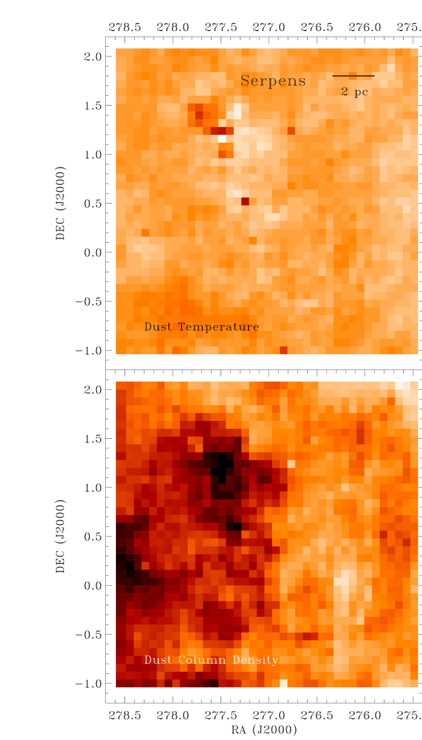
Figure 3: Dust color temperature map (top) and column density map (bottom) of Serpens created from IRIS 60 and 100 $\mu$m images.

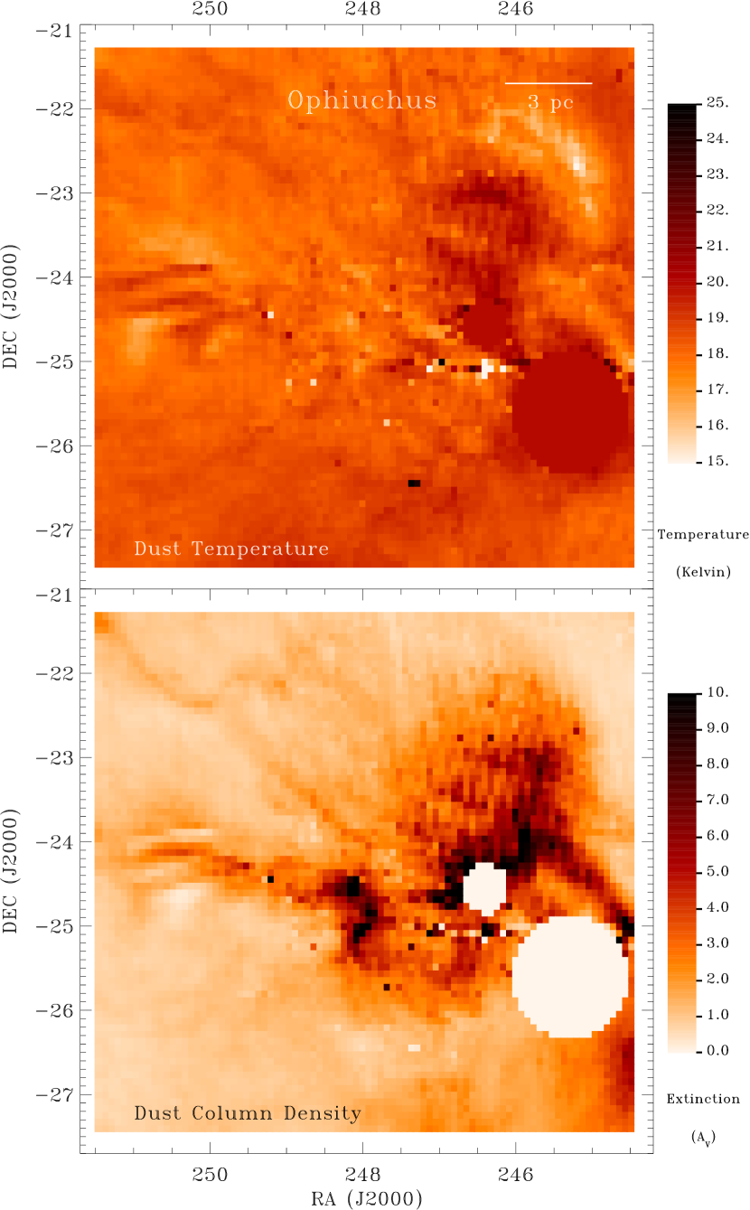
Figure 4: Dust color temperature map (top) and column density map (bottom) of Ophiuchus created from IRIS 60 and 100 $\mu$m images. The two white circles have been excluded due to contamination from B stars.

The dust color temperature and column density maps derived from our parameter fits and IRIS data are among the first publicly available data products distributed by the COMPLETE team. Temperature and extinction maps of Perseus, Ophiuchus and Serpens derived from the IRIS data are shown in Figures 2, 3 and 4. FITS files of these maps can be downloaded from the COMPLETE web page.

In Perseus, there is a striking ring of emission that is centered on a region of warm material. This ring has been discussed by Andersson et al. (2000), Pauls & Schwartz (1989) and Fiedler et al. (1994) and is discussed in more detail in a companion paper to this one (Ridge et al., 2005). The Perseus ring does not stand out in the NICER extinction map as visibly as in the IRIS column density map because it is not a true column density feature. It is difficult to determine from emission maps alone if individual features are the result of changing dust properties or column density enhancements.

A warm dust ring is evident in Ophiuchus in the temperature map, centered at the position 16:25:35, -23:26:50 (J2000). This ring was reported by Bernard, Boulanger & Puget (1993) in a discussion of the far-infrared emission from Ophiuchus and Chameleon, but they did not investigate its nature or possible progenitor. The B star $\rho$-Ophiuchus and a number of X-ray sources are projected to lie within this shell of heated gas. The Ophiuchus ring will be further discussed in a future paper (Li et al., 2005).

5.4 Temperature and Extinction Distributions

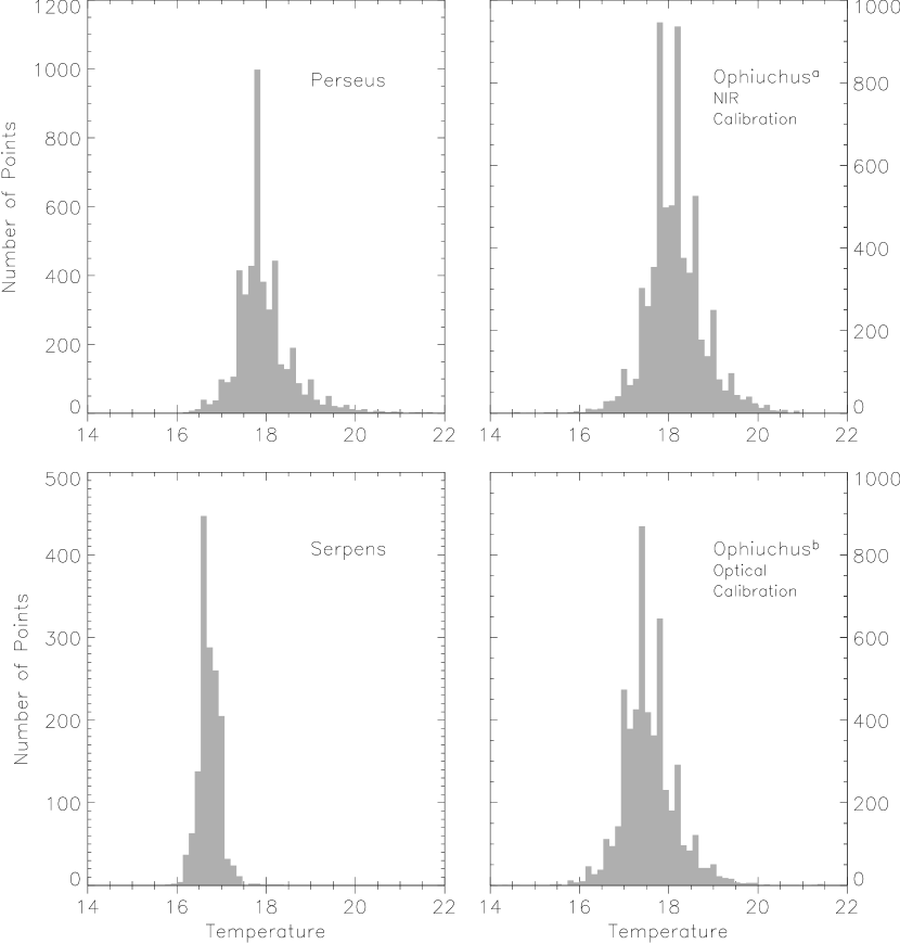
Figure 5: The filled histograms show the temperature derived from the 60/100$\mu$m flux density ratio in Perseus, Serpens and Ophiuchus after the calibration described in Section 2. The Ophiuchus^a histogram (top right) is calibrated to the 2MASS extinction map. The Ophiuchus^b histogram (bottom right) is calibrated to the Cambrésy data.

In Figure 5 we show histograms of the dust temperature in Perseus, Serpens, and Ophiuchus. Each distribution peaks near 17 K, and all except Serpens have a spread of several degrees. The dust temperatures that we derive are, to an extent, calibrated with those derived by Schlegel, Finkbeiner & Davis (1998) (see Section 5.1).

It has been shown for Taurus by Arce & Goodman (1999) that using IRAS 60 and 100 $\mu$m flux densities to determine dust column density gives results consistent with other methods, such as the color excess method (e.g. NICE/NICER), star counts (e.g. Cambrésy (1999)), and using an optical (V and R) version of the average color excess method used by Lada et al. (1994). Here we compare the IRIS derived extinction maps of Perseus, Serpens, and Ophiuchus with maps created by some of these other methods.

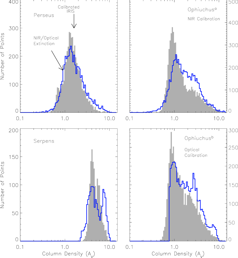
Figure 6: The filled histograms show the extinction derived from the 60/100$\mu$m flux density ratio in Perseus, Serpens and Ophiuchus after the calibration described in Section 2. The blue open histogram shows the NIR/optical derived extinction (from Alves, Lombardi & Foster (2005) and Cambrésy (1999)). The Ophiuchus^a histogram (top right) is calibrated to the 2MASS extinction map. The Ophiuchus^b histogram (bottom right) is calibrated to the Cambrésy data.

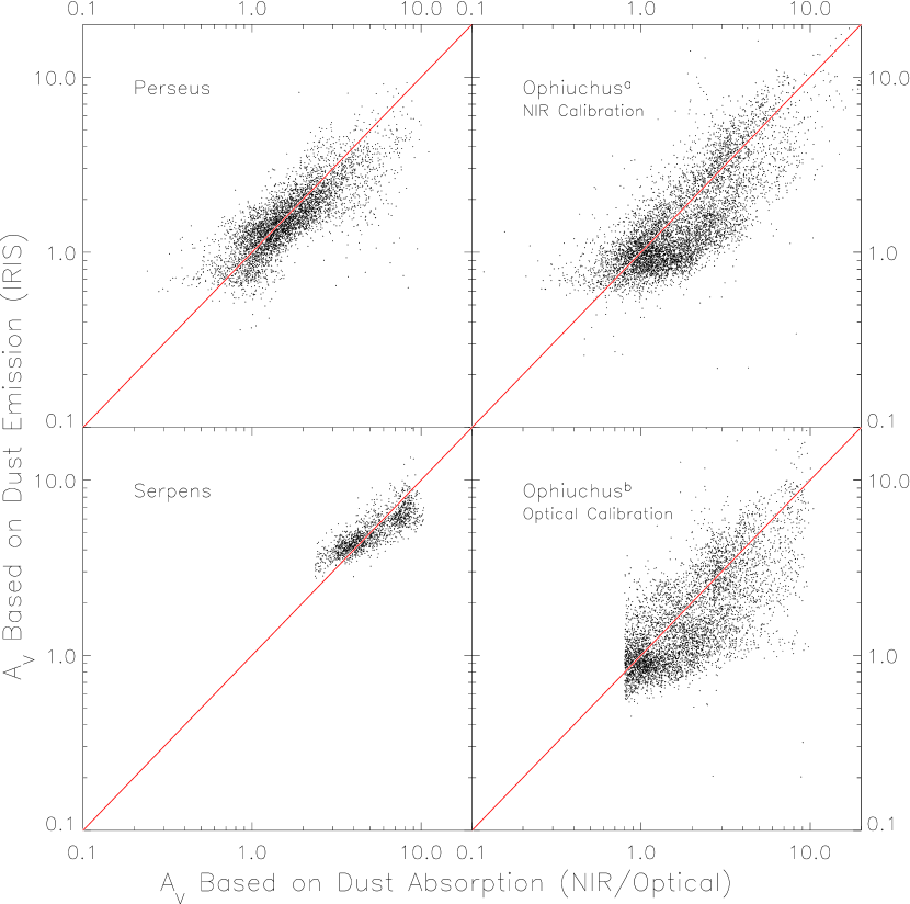
Figure 7: Scatter plot of the corrected IRIS extinction (derived from the 60/100$\mu$m flux density ratio in Perseus, Serpens and Ophiuchus) and the model extinction (from Alves, Lombardi & Foster (2005) and Cambrésy (1999)). The Ophiuchus^a IRIS extinction (top right) is calibrated to the 2MASS extinction map. The Ophiuchus^b IRIS extinction (bottom right) is recalibrated to the Cambrésy data. Note that the data are shown here in log-log plots for clarity of display, but all the fitting is of linear (not log) quantities. The sharp cutoff in the Ophiuchus^b panel is a result of having added 0.71 magnitudes to the optically derived extinction. The sharp cutoff in the Serpens panel is a result of having added 2.2 magnitudes to the optically derived extinction.

Our method requires the FIR-derived extinction to best match the NIR or optical-derived extinction, and the global agreement can be seen in Figure 6. However, the point-to-point extinction values can be significantly different between the two methods, as shown in Figure 7. The large scatter in these extinction plots ($1\sigma\simeq 1$ mag $A_{V}$) is likely the result of the various assumptions used in our calculations. For instance, it is unlikely to be the case that all of the dust along a given line of sight can be well characterized by a single temperature or emissivity spectral index, especially along lines of sight through the denser regions of the molecular clouds. It is also likely that the dust optical depth to visual extinction conversion factor ($X$) is not constant throughout a cloud volume. The flux detected by IRAS comes preferentially from warmer dust, while the extinction maps made from NIR and optical data have no temperature bias, so it is also possible (and in many regions likely) that the dust doing most of the FIR emitting is not the same dust responsible for most of the extinguishing at shorter wavelengths. The scatter for each cloud is shown in Table 3.

As a test to see if the parameters determined for one cloud can be successfully used to describe another, we used the Perseus fits for $\delta$, $\omega$ and $X$ for the Ophiuchus 60 and 100 $\mu$m IRIS maps and compared the derived extinction to the 2MASS extinction map of Ophiuchus. The median point-to-point difference was 0.8 magnitudes of visual extinction, with a standard deviation of 1.9 magnitudes. When the optimized parameters for Ophiuchus are used, the median point-to-point difference is only 0.2 mag, with a scatter of 1.2 mag. We conclude that the fits for one cloud are unlikely to be appropriate for other clouds, and therefore caution should be used in attempts to estimate extinction within molecular clouds from IRAS emission maps alone.

We have derived separate values for $\delta$, $\omega$ and $X$ for various regions within Perseus to see if the dust properties are significantly different there than in the cloud as a whole. The regions considered were B5, IC348, NGC1333, the emission ring, and the area surveyed by the c2d Spitzer Legacy project. The locations and sizes of the Perseus sub-regions are shown in Table 1. The values of $\delta$, $\omega$ and $X$ for these sub-regions are shown in Table 2 and displayed in Figure 2. The value of $\delta$ varies by about 10 percent, $\omega$ varies by about 20 percent and $X$ varies by 20 percent in these sub-regions of Perseus. NGC1333 varies much more significantly from the other sub-regions of Perseus.

We conclude that the method described here for converting dust emission to visual extinction can be used with confidence to find regions with high or low extinction and to determine the average extinction in large areas ($\sim$0.25 square degrees). However, the extinction determined in any individual 5′ pixel should not be trusted to represent the true absolute extinction to better than $\sim$ 2.5 magnitudes (2$\sigma$) of visual extinction. This is made clear by the significant variability in the emissivity spectral index of dust and the conversion from dust optical depth to visual extinction between clouds and within clouds, as shown in Tables 2 and 3.

5.5 Emissivity Spectral Index

The emissivity spectral index that we use in this paper varies with temperature as shown in Equation 2. The values that we find for the parameters $\delta$ and $\omega$ are shown in Table 2. Their values as determined by Dupac et al. (2003) are 0.4 and 0.008 respectively, which comes from a much broader range of environments and many more measurements of the FIR/sub-mm flux. Figure 8 shows the emissivity spectral index that we find for each cloud plotted along with the curve from Dupac et al. (2003). The emissivity spectral index is considerably larger in Ophiuchus than in Serpens, which is somewhat higher than $\beta$ in Perseus. The best-fit curve to the wider range of environments in Dupac et al. (2003) falls between our Serpens and Ophiuchus curves.

6 Summary

We have described a new method that uses NIR color excesses or optical star counts to constrain the conversion of IRIS 60 and 100 $\mu$m data into color temperature and column density maps. Our method also derives the dust emissivity spectral index and the conversion from dust 100 µm optical depth to visual extinction. We test the IRIS 60 and 100 µm zero points and confirm that, unlike earlier releases of IRAS data, the IRIS recalibration is properly zero point corrected. We find the the very small grain contribution to the 60 µm flux is significant.

The dust temperature maps of Perseus, Serpens and Ophiuchus available through the COMPLETE website should be the best dust temperature maps of large star forming regions at 5′ resolution created to date. The dust temperatures derived here are dependent on the emissivity spectral index of the dust, which is solved globally for each molecular cloud, and recorded in Table 2.

Our work here indicates that one can not confidently convert dust 100 µm optical depth to visual extinction without the benefit of having an extinction map made in an alternative manner to use as a model because the conversion constant $X$ varies significantly from cloud to cloud, and even within a cloud (see Table 2). Using the values for the dust emissivity spectral index and visual extinction conversion derived for one cloud results in a significant miscalculation of the extinction in other clouds. Even with the NICER and optical star counting extinction maps used here to calibrate the IRAS data, there is significant point-to-point variation between the two estimates (see Figure 1). In fact, we have shown that in Ophiuchus the optical star count method employed by Cambrésy (1999) has an offset from the NICER method applied to the 2MASS data set of $\sim$ 0.71 magnitudes in A_V, with a scatter of 0.7 magnitudes, so the issue is not simply one of dealing with the FIR dust properties in molecular clouds.

In addition, we have identified two ring structures, one in Perseus and one in Ophiuchus, which are discussed in upcoming papers (Ridge et al., 2005) and (Li et al., 2005) respectively.

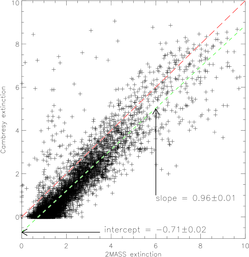
Figure 1: Scatter plot of the Ophiuchus optical star counting (Cambrésy, 1999) and NIR color excess method (Alves, Lombardi & Foster, 2005) extinctions in Ophiuchus. The green line (short dashes) is the best fit line to the data sets, with the equation shown at bottom of the image. The red (1:1) line (long dashes) is there only to guide the eye. Nearly 60 percent of the data points have 2MASS extinctions less than 2.

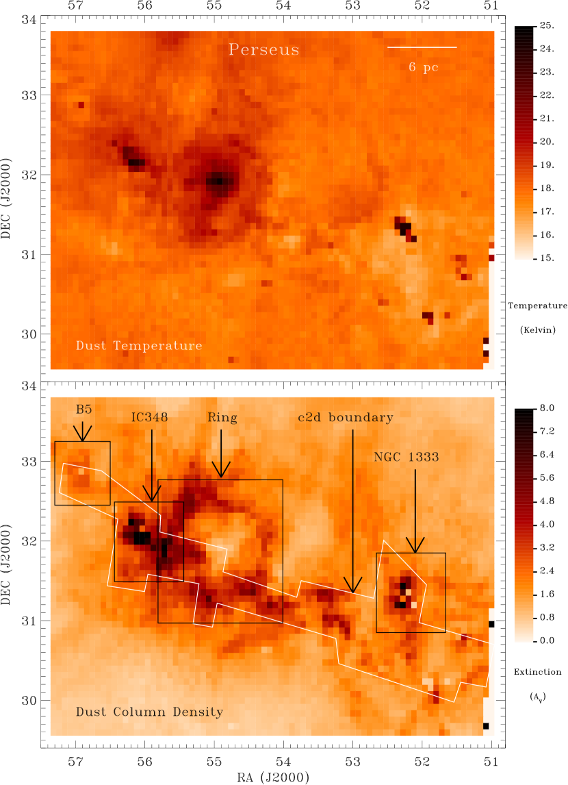
Figure 2: Dust color temperature map (top) and column density map (bottom) of Perseus created from IRIS 60 and 100 $\mu$m images.

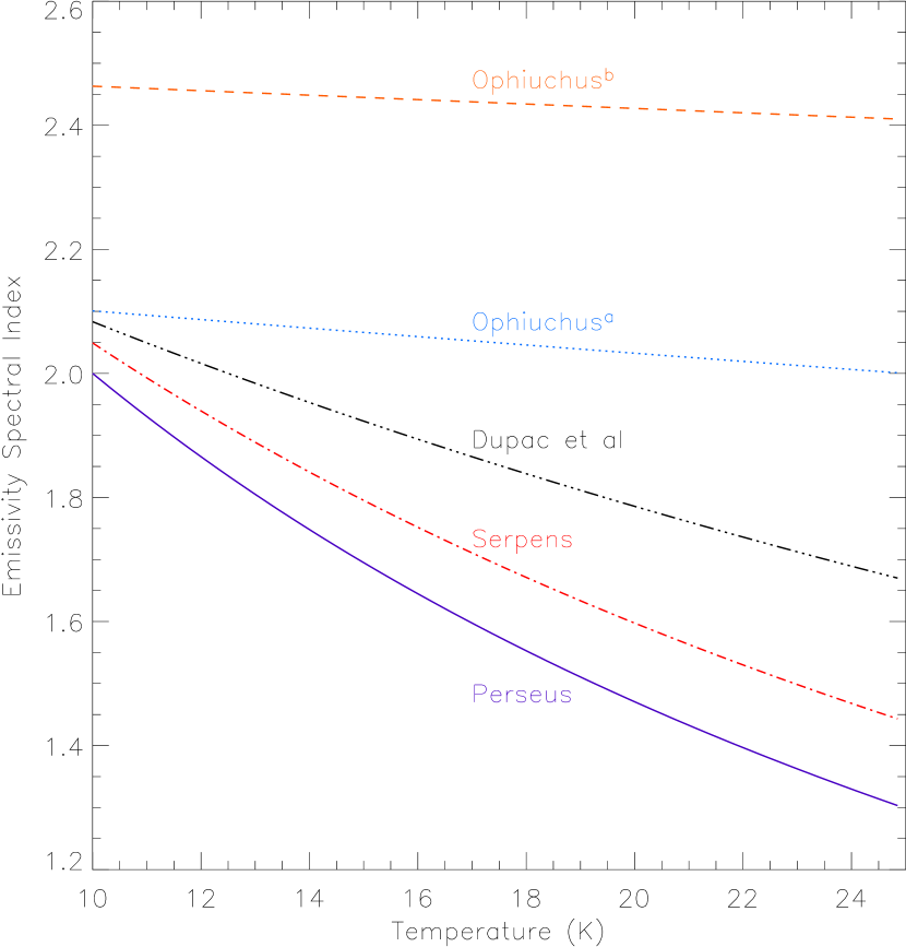
Figure 8: Plot of the emissivity spectral index versus temperature for Perseus, Ophiuchus and Serpens. The Ophiuchus^a curve is for the IRIS data calibrated to the 2MASS extinction map. The Ophiuchus^b curve is calibrated to the Cambrésy data. The Dupac et al curve is the best fit curve to a collection of FIR/sub-mm emission regions as presented in Dupac et al. (2003).

Table 1: IRIS Image Details

Region	Center RA	Center Dec	Image Size
	(degrees)	(degrees)	(degrees)
Perseus	54.30	31.85	6.6$\times$4.5
Perseus Ring	54.91	31.87	1.8$\times$1.8
B5	56.90	32.85	0.8$\times$0.8
IC348	55.94	31.99	1.0$\times$1.0
NGC1333	52.16	31.35	1.0$\times$1.0
Ophiuchus	247.95	-24.00	6.9$\times$6.8
Serpens	277.00	0.50	3.0$\times$3.0

Note. — All positions are given in equatorial J2000 equinox coordinates.

Table 2: Best Fit IRAS/dust Parameters

Cloud	$\delta$	$\omega$	$X$	$A_{V}$ offset
				(mag $A_{V}$)
Perseus	0.32	0.0180	1100	–
B5	0.38	0.0140	1200	–
IC348	0.33	0.0160	1000	–
NGC1333	0.64	0.0010	1300	–
c2d Area	0.36	0.0140	1200	–
Ring	0.38	0.0150	990	–
Ophiuchus	0.46	0.0016	510	–
Ophiuchus	0.40	0.0006	350	0.71
Serpens	0.35	0.0139	800	2.36

Note. — Best fit values for the parameters used to convert IRIS flux to visual extinction

Table 3: Scatter between IRAS implied extinction and NIR/optical derived extinction

Cloud	Median Difference	1$\sigma$ Scatter Between Methods	Scatter Between Methods	$\tau_{100}$/$A_{V}$
	(mag $A_{V}$)	(mag $A_{V}$)	Percent	10-4 mag-1
Perseus	-0.1	0.9	30	9 $\pm$ 3
Ophiuchus	-0.2	1.2	50	17 $\pm$ 9
Ophiuchus	-0.2	1.4	50	23 $\pm$ 13
Serpens	0.0	1.2	20	12 $\pm$ 3

Note. — Median difference between the different ways to estimate extinction within a molecular cloud (IRIS $A_{V}$ - NIR/optical $A_{V}$), and the scatter between the methods (see Section 5.4).

References

- Abergel et al. (1994) Abergel, A., Boulanger, F., Mizuno, A., & Fukui, Y. 1994, ApJ, 423, L59
- Andersson et al. (2000) Andersson, B.-G., Wannier, P. G., Moriarty-Schieven, G. H., & Bakker, E. J. 2000, AJ, 119, 1325
- Alves, Lombardi & Foster (2005) Alves, J., Lombari, M., & Foster, J. In prep.
- Arce & Goodman (1999) Arce, H. G. & Goodman, A. A. 1999, ApJ, 517, 264
- Arce & Goodman (1999) Arce, H. G. & Goodman, A. A. 1999, ApJ, 512, L135
- Bernard, Boulanger & Puget (1993) Bernard, J. P., Boulanger, F., & Puget, J. L. 1993, A&A, 277, 609
- Boulanger et al. (1998) Boulanger, F., Bronfman, L., Dame, T. M., & Thaddeus, P. 1998, A&A, 332, 273
- Cambrésy (1999) Cambrésy, L. 1999, A&A, 345, 965
- Cambrésy et al. (2005) Cambrésy, L., Jarrett, T. H., & Beichman, C. A. 2005, A&A, 435, 131
- Désert et al. (1990) Désert, F.-X., Boulanger, F., & Puget, J. L. 1990, A&A, 237, 215
- Dupac et al. (2003) Dupac, X., et al. 2003, A&A, 404, L11
- Evans et al. (2003) Evans, N. J., et al. 2003, PASP, 115, 965
- Fiedler et al. (1994) Fiedler, R., Pauls, T., Johnston, K. J., & Dennison, B. 1994, ApJ, 430, 595
- Goodman (2004) Goodman, A. A. 2004, ASP Conf. Ser. 323: Star Formation in the Interstellar Medium: In Honor of David Hollenbach, 323, 171
- Jarrett, Dickman & Herbst (1989) Jarrett, T. H., Dickman, R. L., & Herbst, W. 1989, ApJ, 345, 881
- Lada et al. (1994) Lada, C. J., Lada, E. A., Clemens, D. P., & Bally, J. 1994, ApJ, 429, 694
- Lagache et al. (1998) Lagache, G., Abergel, A., Boulanger, F., & Puget, J.-L. 1998, A&A, 333, 709
- Laureijs et al. (1991) Laureijs, R. J., Clark, F. O., & Prusti, T. 1991, ApJ, 372, 185
- Li et al. (2005) Li, D., Goodman, A. A., Ridge, N., & Schnee, S. In prep.
- Lombardi & Alves (2001) Lombardi, M., & Alves, J. 2001, A&A, 377, 1023
- Miville-Deschênes & Lagache (2005) Miville-Deschênes, M., & Lagache, G. 2005, ApJS, 157, 302
- Monet (1996) Monet, D. 1996, BAAS, 188, 5404
- Nagata et al. (2002) Nagata, H., Shibai, H., Takeuchi, T. T., & Onaka, T. 2002, PASJ, 54, 695
- Nelder & Meade (1965) Nelder, J. & Meade, R. 1965, Computer Journal, 7, 308
- Pauls & Schwartz (1989) Pauls, T., & Schwartz, P. R. 1989, in The Physics and Chemistry of Interstellar Molecular Clouds, ed G.W. . T.J. Armstrong (Berlin: Springer), 225
- Ridge et al. (2005) Ridge, N., Schnee, S., & Goodman, A. A. Submitted to ApJ
- Schlegel, Finkbeiner & Davis (1998) Schlegel, D. J., Finkbeiner, D. P., & Davis, M. 1998, ApJ, 500, 525
- Wood, Myers & Daugherty (1994) Wood, D. O. S., Myers, P. C., & Daugherty, D. A. 1994, ApJS, 95, 457