New Type of Magneto-Rotational Instability in Cylindrical Taylor-Couette Flow

Abstract

We study the stability of cylindrical Taylor-Couette flow in the presence of combined axial and azimuthal magnetic fields, and show that adding an azimuthal field profoundly alters the previous results for purely axial fields. For small magnetic Prandtl numbers $Pm$, the critical Reynolds number $Re_{c}$ for the onset of the magneto-rotational instability becomes independent of $Pm$, whereas for purely axial fields it scales as $Pm^{-1}$. For typical liquid metals, $Re_{c}$ is then reduced by several orders of magnitude, enough that this new design should succeed in realizing this instability in the laboratory.

The magneto-rotational instability (MRI) is one of the most important processes in astrophysics, with applications ranging from accretion disks to entire galaxies r1 ; r2 . There is therefore great interest in trying to study this instability in the laboratory r3 ; r4 ; r5 ; r6 ; r7 ; r8 ; r9 ; r10 . These experiments are complicated by the extremely small magnetic Prandtl numbers of liquid metals, which necessitate very large rotation rates. Here we report on a new type of magneto-rotational instability, that operates even at infinitesimal Prandtl number, and correspondingly at far lower rotation rates. This new instability should be much easier to obtain experimentally, and may also have considerable astrophysical implications.

The magneto-rotational instability is a mechanism for transporting angular momentum. Consider, for example, an accretion disk around a newly forming star. In order for material to fall inward, it must transfer its angular momentum to material further out. The difficulty is how to accomplish this. In particular, a Keplerian angular velocity profile, for which $\Omega\sim r^{-3/2}$, is known to be hydrodynamically stable (at least linearly), by the familiar Rayleigh criterion. Purely viscous coupling in a laminar flow is many orders of magnitude too small though; if this were the angular momentum transport mechanism, stars would take so long to form that none would yet exist today, some 14 billion years after the Big Bang.

This conundrum was solved by Balbus & Hawley r1 , who showed that such a Keplerian profile may be hydrodynamically stable, but is nevertheless magnetohydrodynamically unstable. The addition of a magnetic field opens up a new way of coupling fluid parcels, namely via the magnetic tension in the field lines, and thereby allows for a new instability, the magneto-rotational instability, that has no analog in the purely hydrodynamic problem. Coupling the fluid in this way is then so much more efficient at transporting angular momentum that this mechanism can indeed yield accretion rates more in line with those observed. Something as basic as the time it takes for a star to form is thus magnetically controlled.

Subsequent to this work, it was soon realized that this instability had actually been discovered decades earlier, by Velikhov r11 , who had not considered it in an astrophysical context though. Instead, he had viewed it simply as the magnetohydrodynamic extension of the so-called Taylor-Couette problem, consisting of the flow between differentially rotating cylinders. See for example r12 for a review of this problem, one of the oldest in fluid dynamics.

Once the connection is made to the classical Taylor-Couette problem, one immediately recognizes that this should be a way to study this instability in the lab: just take the fluid to be a liquid metal, and apply a magnetic field along the cylinders. This simple design is the basis of most of the MRI experiments proposed to date r3 ; r4 ; r5 ; r6 ; r7 ; r8 . (Sisan et al. r9 claim to have obtained the magneto-rotational instability already, in spherical rather than cylindrical geometry. However, there are enough other instabilities that can arise in this configuration, e.g. r13 , that their results are also open to other interpretations. Indeed, the basic state from which their instability arises is already fully turbulent, indicating that whatever their instability may be, it is certainly not the first instability to set in.)

As simple as it sounds, there is unfortunately also one considerable difficulty associated with these experiments, namely that the rotation rates of the inner and outer cylinders must be enormous. The problem is that the relevant parameter is not so much the hydrodynamic Reynolds number $Re=\Omega_{i}r_{i}^{2}/\nu$, but rather the magnetic Reynolds number $Rm=\Omega_{i}r_{i}^{2}/\eta$, where $\nu$ is the viscosity and $\eta$ the magnetic diffusivity. In its traditional form, the magneto-rotational instability sets in when $Rm=O(10)$. $Re$ is then given by $Rm/Pm$, where $Pm=\nu/\eta$ is the magnetic Prandtl number, a material property of the fluid. Typical values are $\sim$$10^{-5}$ for liquid sodium, $\sim$$10^{-6}$ for gallium, and $\sim$$10^{-7}$ for mercury. $Re$ must therefore be at least $10^{6}$, and possibly larger still, depending on the particular liquid metal one intends to use.

Such large values can be reached in the lab; taking the inner cylinder radius $r_{i}=10$ cm, say, one finds that rotation rates of around 10 Hz are required – large, but achievable. The difficulty lies elsewhere, namely in the ends that would necessarily be present in any real experiment. Due to the Taylor-Proudman theorem, stating that in rapidly rotating systems the flow will tend to align itself along the axis of rotation, end-effects become increasingly important, until at $Re=O(10^{6})$ the flow is controlled almost entirely by the end-plates r14 . That is, while it is possible to achieve such large rotation rates, the flow will look nothing like the idealized infinite-cylinder flow on which all of the theoretical analysis is based.

A new approach is therefore needed if this instability is to be studied in the laboratory. We propose the following: instead of imposing only a uniform axial field $B_{z}=B_{0}$, additionally also impose an azimuthal field $B_{\phi}=\beta B_{0}(r_{i}/r)$, where $\beta$ is a nondimensional measure of the relative magnitudes of $B_{\phi}$ and $B_{z}$, and the dimensional quantity $B_{0}$ will be incorporated into the Hartmann number below. Such a $B_{\phi}$ field can be generated just as easily as a $B_{z}$ field, by running a current-carrying wire down the axis of the inner cylinder (suitably insulated from the fluid, of course). Note also that with neither $B_{z}$ nor $B_{\phi}$ maintained by currents within the fluid itself, the possibility of magnetic instabilities is excluded a priori. The only source of energy to drive an instability is the imposed differential rotation; the magnetic field merely acts as a catalyst.

Given this basic state consisting of these externally imposed magnetic fields, as well as the differential rotation profile $\Omega(r)$ imposed by the rotation rates $\Omega_{i}$ and $\Omega_{o}$ of the two cylinders, we linearize the governing equations about it, and look for axisymmetric disturbances. These are known to be preferred over non-axisymmetric ones for the classical $\beta=0$ MRI, and are therefore the appropriate starting point here as well. The perturbation flow and field may then be expressed as

$${\bf u}=v{\bf\hat{e}}_{\phi}+\nabla\times(\psi{\bf\hat{e}}_{\phi}),\qquad{\bf b}=b{\bf\hat{e}}_{\phi}+\nabla\times(a{\bf\hat{e}}_{\phi}).$$

Taking the $z$ and $t$ dependence to be $\exp(ikz+\gamma t)$, the perturbation equations become

$$Re\,\gamma\,v=D^{2}v+Re\,ik\,r^{-1}(r^{2}\Omega)^{\prime}\,\psi+H\!a^{2}\,ik\,b,$$

$$Re\,\gamma\,D^{2}\psi=D^{4}\psi-Re\,2ik\,\Omega\,v+H\!a^{2}\,ik(D^{2}a+2\beta r^{-2}b),$$

$$Pm\,Re\,\gamma\,b=D^{2}b-Pm\,Re\,ik\,\Omega^{\prime}r\,a+ik\,v-2ik\,\beta r^{-2}\psi,$$

$$Pm\,Re\,\gamma\,a=D^{2}a+ik\,\psi,$$

where $D^{2}=\nabla^{2}-1/r^{2}$, and the primes denote $d/dr$.

Length has been scaled by $r_{i}$, time by $\Omega_{i}^{-1}$, $\Omega$ by $\Omega_{i}$, $\bf u$ by $\eta/r_{i}$, and ${\bf B}_{0}$ and $\bf b$ by $B_{0}$. The various nondimensional parameters are then: (a) the magnetic Prandtl number $Pm=\nu/\eta$ already mentioned above, (b) the ratio $\hat{\mu}=\Omega_{o}/\Omega_{i}$ (this enters into the details of $\Omega(r)=c_{1}+c_{2}/r^{2}$) and the Reynolds number $Re=\Omega_{i}r_{i}^{2}/\nu$, measuring the relative and absolute rotation rates of the two cylinders, (c) the parameter $\beta$ and the Hartmann number $H\!a=B_{0}r_{i}/\sqrt{\rho\mu\eta\nu}$ ($\rho$ is the fluid’s density, $\mu$ the magnetic permeability), measuring the relative and absolute magnitudes of the imposed magnetic fields, and (d) the radius ratio $r_{i}/r_{o}$, which we fixed at $1/2$.

The radial structure of $v$, $\psi$, $b$ and $a$ was expanded in terms of Chebyshev polynomials, typically up to $N=40-80$. These equations and associated boundary conditions (no-slip for $\bf u$, insulating for $\bf b$) then reduce to a large ($4N$ by $4N$) matrix eigenvalue problem, with the eigenvalue being the growth or decay rate $\gamma$ of the given mode. Note also that this numerical implementation is very different from that of r4 , in which the individual components of $\bf u$ and $\bf b$ were used, and discretized in $r$ by finite differencing. Both codes yielded identical results though in every instance where we benchmarked one against the other.

The following sequence of calculations was then carried out. First, we fixed $Pm$, $\beta$ and $\hat{\mu}$, and scanned through a range of values of $Re$, $H\!a$ and $k$, in each case determining whether the given modes grow or decay. We thus found the smallest value of $Re$, and the corresponding $H\!a$ and $k$, that yields a marginally stable solution, one having Re$(\gamma)=0$ (which typically involved solving the basic eigenvalue problem for several thousand combinations of $Re$, $H\!a$ and $k$). By repeating this entire procedure for different values of $Pm$, $\beta$ and $\hat{\mu}$, we obtained the results in Fig. 1.

The dotted curve to the left of $\hat{\mu}=0.25$ is a purely hydrodynamic instability, namely the onset of Taylor vortices, e.g. r12 . As we approach $\hat{\mu}=0.25$ though, we note that $Re_{c}\to\infty$. This critical value $\hat{\mu}=0.25$ ($(r_{i}/r_{o})^{2}$, in general) is precisely the so-called Rayleigh line, beyond which the flow is hydrodynamically stable, because the angular momentum increases outward.

We are more interested therefore in the behavior to the right of $\hat{\mu}=0.25$, where we anticipate that the inclusion of magnetic effects will yield the MRI. We begin with the two curves $\beta=0$, the MRI as it has been considered to date r10 . We see how $Re_{c}$ rises very steeply from the previous nonmagnetic results to the left of $\hat{\mu}=0.25$, and then scales as $Pm^{-1}$, exactly as described above, and in perfect agreement with r4 . And again, because $Pm$ is so small, these values end up being too large for the experiment to succeed r14 .

However, turning next to the results for non-zero $\beta$, we see that $Re_{c}$ is dramatically reduced, over a range of $\hat{\mu}$ extending increasingly far beyond the Rayleigh line. For example, if we focus on how far we can go before $Re_{c}=10^{4}$, say, we obtain $\hat{\mu}=0.253$, 0.264, 0.292 and 0.308 for $\beta=1$, 2, 4 and 8, respectively. Furthermore, within these $\hat{\mu}$ ranges $Re_{c}$ is independent of $Pm$, very different from the previous $Pm^{-1}$ scaling. Indeed, within these ranges one can set $Pm=0$ and still obtain exactly the same solutions. This $Pm=0$ limit was considered before by Chandrasekhar r15 , but for axial fields only, in which case there are no instabilities to the right of the Rayleigh line.

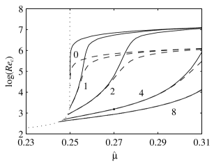
Figure 1: The critical Reynolds number $Re_{c}$ as a function of $\hat{\mu}$. The dotted curve to the left of $\hat{\mu}=0.25$ is a purely nonmagnetic instability. The curves to the right of $\hat{\mu}=0.25$ are the magneto-rotational instability. Solid curves are $Pm=10^{-6}$, dashed curves $Pm=10^{-5}$. The numbers beside pairs of curves indicate $\beta$. Finally, the dot on the $\beta=4$ curves corresponds to the solution shown in Fig. 2.

The explanation for this very different behavior for non-zero $\beta$ lies in the coupling between the azimuthal field $b$ and the meridional circulation $\psi$. If $\beta=0$ these quantities are not directly coupled at all, only indirectly through $v$ and $a$. For non-zero $\beta$ each acts directly on the other. Of these two new terms in the equations, the more important one turns out to be the effect of $\psi$ on $b$. Physically, this corresponds to the meridional circulation $\psi$ advecting the original $B_{\phi}$ and thereby generating a contribution to $b$. It is this new way of maintaining $b$ that allows this instability to proceed even in the $Pm=0$ limit, where the classical $\beta=0$ MRI fails.

Figure 2 shows an example of these new solutions. We note that however dramatically $Re_{c}$ may have been reduced, the spatial structure is much the same as for $\beta=0$, consisting of Taylor vortices elongated slightly in the $z$-direction. There is actually one subtle difference, namely that the up/down symmetry in $z$ has been broken. This is due to the handedness of the imposed field, which distinguishes between $\pm z$ in a way that a purely axial field does not. As a result of this symmetry-breaking, these new modes are also no longer stationary, but instead have Im$(\gamma)\neq 0$, corresponding to a drift in $z$, at the rate Im$(\gamma)/k$. This particular solution has Im$(\gamma)=0.153$ and $k=2.33$, for a drift rate of $0.066\,(r_{i}\Omega_{i})$.

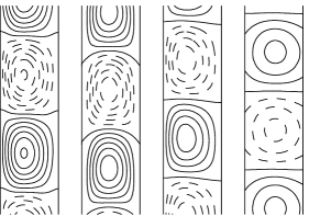
Figure 2: The spatial structure of the eigenmode for $Pm=0$, $\beta=4$ and $\hat{\mu}=0.27$, for which $Re_{c}=1521$ (see Fig. 1), $H\!a=16.3$ and $k=2.33$. From left to right, contours of $v$, $\psi$, $b$ and $a$, with the contour interval for $b$ and $a$ 1/3 that of $v$ and $\psi$. Note the lack of any particular phase relationship between the various quantities, due to the $\pm z$ symmetry-breaking.

Turning next to the Hartmann number $H\!a=16.3$, this translates into a $\sim$12 G field, taking the fluid to be liquid sodium, and $r_{i}=10$ cm. An axial field of that magnitude is certainly easily achievable in the lab. For the azimuthal field we then want 500 G cm/$r$, corresponding to a current of 2500 A in this wire running down the central axis, which is again achievable, if perhaps not quite so easily.

To summarize then, we have shown that the magneto-rotational instability is radically altered if one imposes both axial and azimuthal magnetic fields, becoming independent of the magnetic Prandtl number in the $Pm\to 0$ limit – a result that is all the more remarkable as neither purely axial nor purely azimuthal fields yield anything like it. With this new scaling, the critical Reynolds numbers are reduced by several orders of magnitude, enough that these instabilities could perhaps be attainable in the lab without being disrupted by end-effects (although of course some end-effects will always be present, particularly with this slow drift in $z$). Further computational work includes the nonlinear equilibration of these modes, as well as the possibility of non-axisymmetric instabilities. These and other issues are currently being explored.

Finally, returning briefly to the original astrophysical motivation, we note that virtually all astrophysical bodies do in fact have both axial and azimuthal magnetic fields. These magnetic fields are typically not externally imposed though, but rather generated by electric currents flowing within the system itself. Self-consistently solving for both the large-scale fields as well as the small-scale instabilities is then far more complicated than our analysis here, but the basic ingredients are certainly there for this new type of magneto-rotational instability to play a role.

- (1) S. A. Balbus and J. F. Hawley, Astrophys. J. 376, 214 (1991).
- (2) S. A. Balbus, Ann. Rev. Astron. Astrophys. 41, 555 (2003).
- (3) G. Rüdiger and Y. Zhang, Astron. Astrophys. 378, 302 (2001).
- (4) G. Rüdiger, M. Schultz, and D. Shalybkov, Phys Rev. E 67, art no 046312 (2003).
- (5) H. T. Ji, J. Goodman, and A. Kageyama, Mon. Not. Roy. Astron. Soc. 325, L1 (2001).
- (6) A. Kageyama, H. T. Ji, J. Goodman, F. Chen, and E. Shoshan, J. Phys. Soc. Japan 73, 2424 (2004).
- (7) A. P. Willis and C. F. Barenghi, Astron. Astrophys. 388, 688 (2002).
- (8) K. Noguchi, V. I. Pariev, S. A. Colgate, H. F. Beckley, and J. Nordhaus, Astrophys. J. 575, 1151 (2002).
- (9) D. R. Sisan, N. Mujica, W. A. Tillotson, Y. M. Huang, W. Dorland, A. B. Hassam, T. M. Antonsen, and D. P. Lathrop, Phys. Rev. Lett. 93, art no 114502 (2004).
- (10) R. Rosner, G. Rüdiger, and A. Bonanno, Eds., MHD Couette Flows: Experiments and Models, American Inst. Phys. Conf. Proc. vol 733 (2004).
- (11) E. P. Velikhov, Sov. Phys. JETP 36, 995 (1959).
- (12) R. Tagg, Nonlin. Science Today 4, 1 (1994).
- (13) R. Hollerbach and S. Skinner, Proc. Roy. Soc. London A 457, 785 (2001).
- (14) R. Hollerbach and A. Fournier, In [10], pp. 114–121. See also http://arxiv.org/abs/astro-ph/0506081
- (15) S. Chandrasekhar, Hydrodynamic and Hydromagnetic Stability, Oxford University Press (1961).