The stellar population and interstellar medium in NGC 6822

Abstract

We present a comprehensive study of the stellar population and the interstellar medium in NGC 6822 using high-quality Hi data (obtained with the Australia Telescope Compact Array) and optical broad/narrow-band data (obtained with Subaru and the INT). Our H$\alpha$ observations are an order of magnitude deeper than previous studies and reveal a complex filamentary network covering almost the entire central disk of NGC 6822. We find hitherto unknown Hii regions in the outskirts of NGC 6822 and the companion galaxy. The old and intermediate age stellar population can be traced out to radii of over 0.6^∘ ($>5$ kpc), significantly more extended than the HI disk. In sharp contrast, the distribution of the young, blue stars, closely follows the distribution of the Hi disk and displays a highly structured morphology.

We find evidence for an older stellar population in the companion galaxy – the current star formation activity, although likely to have been triggered by the interaction with NGC 6822, is not the first star formation episode in this object. We show that the properties of the giant kpc-sized hole in the outer Hi disk of NGC 6822 are consistent with it being formed by the effects of stellar evolution.

1. Introduction

Dwarf irregular galaxies are ideal laboratories to study galaxy evolution. Their relatively simple structure, without dominant spiral arms, bulges, and other complicating properties make it more straight-forward to study the various physical processes related to star formation occuring in these galaxies. Their low metallicities and gas-richness suggest that they are still in an early stage of their conversion from gas into stars.

NGC 6822 is one of the closest gas-rich dwarfs in the Local Group. Discovered by Barnard (1884), it was studied in detail by Hubble (1925) who showed that its distance placed it well outside our Milky Way galaxy, making NGC 6822 the first object to be recognized as an “extra-galactic” system (see also Perrine 1922). NGC 6822 is not associated with any of the subgroups in the Local Group (Mateo, 1998; van den Bergh, 1999) but is a member of an extended cloud of irregulars known as the “Local Group Cloud” (Mateo, 1998).

Due to the small distance of $490\pm 40$ kpc (Mateo, 1998) the galaxy appears very extended on the sky: its optical angular diameter is over a quarter of a degree; the Hi disk measures close to a degree (de Blok & Walter, 2000). The galaxy has a total luminosity of $M_{B}\!=\!-15.8$ (Hodge et al., 1991) and a total Hi mass of $1.3\times 10^{8}\ M_{\odot}$ (de Blok & Walter 2000; this work), making it relatively gas-rich. It is a metal poor galaxy, with an ISM abundance of about 0.2 $Z_{\odot}$ (Skillman et al., 1989) and has a star formation rate of $\sim 0.06\ M_{\odot}{\rm yr}^{-1}$ (based on H$\alpha$ and FIR fluxes; Mateo 1998; Israel et al. 1996). Hodge (1980) found evidence for increased star formation between 75 and 100 Myr ago, while Gallart et al. (1996b) showed that the star formation in NGC 6822 increased by a factor of 2 to 6 between 100 and 200 Myr ago. Wyder (2003), from HST imaging, found a spatially variable recent star formation rate in the central parts of NGC 6822. This is all consistent with the mostly constant but stochastic recent star formation histories often derived for dwarf and LSB galaxies. NGC 6822 can be regarded as a rather average and quiescent dwarf irregular galaxy.

Recent optical studies have concentrated on the extended stellar disk of NGC 6822. de Blok & Walter (2003), Battinelli, Demers, & Letarte (2003) and Komiyama et al. (2003) all found that the stellar disk of NGC 6822 extends much further out than the conventional optical appearance suggests. Significant numbers of young stars were found throughout the entire Hi disk. Its inclination, gas-richness and proximity make it an ideal candidate for studying the rotation curve, dark matter content (Weldrake, de Blok, & Walter, 2003) and relation between the stellar population and gaseous ISM. This is a major motivation for this study of the stellar populations and neutral interstellar medium of NGC 6822.

In this paper we present the full Hi data set used earlier in de Blok & Walter (2000) and de Blok & Walter (2003). We re-analyse the Subaru optical data sets described in Komiyama et al. (2003), reaching significantly fainter limiting magnitudes. We discuss the distribution of the old and young stellar populations, and find that NGC 6822 is surrounded by a stellar halo measuring at least a degree in extent. We discuss new deep, wide-field H$\alpha$ images of the entire Hi disk, and find several faint hitherto unknown Hii regions in the outer parts of NGC 6822, including in the NW cloud and on the far rim of the giant hole. Finally, we study the stellar population in the giant hole and find clear evidence for an age gradient, consistent with the idea that star formation is capable of forming giant kpc-sized holes in the ISM. In a companion paper [de Blok & Walter 2005 (Paper II)] we use the data sets presented here to study in detail the star formation threshold in NGC 6822.

In Sections 2, 3 and 4 we describe the various data sets used. Section 5 deals with the stellar populations in NGC 6822, and their relative distributions. There we also discuss the properties of the NW cloud as well as the evolutionary history of the prominent super-giant shell. In Sect. 6 we summarise our results.

2. HI Observations

2.1. Single Dish

NGC 6822 was observed on 16 December 1998 using the ATNF Parkes single-dish telescope in Australia. The narrow-band back-end system (Haynes et al., 1998) of the Multi-Beam system (Staveley-Smith et al., 1996) was used. This set-up uses the central 7 beams. A band width of 4 MHz with 1024 channels and a velocity spacing of 0.8 km s^-1 was used.

An area of $4\times 4$ degrees was observed by scanning the telescope over the sky at a rate of 1 degree per minute, outputting 14 spectra (7 beams $\times$ 2 polarizations) every 5 seconds. Frequency switching was used to determine the bandpass correction. The system temperature was 24 K.

The individual bandpass-corrected single-beam, single-polarization spectra were gridded into a data cube of 4.5 $\times$ 4.5 degrees $\times$ 820 km s^-1 with a pixel size of 4${}^{\prime}\times 4^{\prime}\times 1.6$ km s^-1. The effective beam size was 16.7^′ (2.5 kpc). The total integration time per point was $\sim 35$ s per polarization, resulting in a noise of 0.08 Jy beam^-1 per channel. The corresponding column density sensitivity is $\sim 1.0\cdot 10^{17}$ cm^-2 per 1.6 $\,\mbox{km}\,\mbox{s}^{-1}$ channel for emission filling the beam. These numbers are summarised in Table 1.

With a systemic velocity of $-55$ $\,\mbox{km}\,\mbox{s}^{-1}$, the Hi emission from NGC 6822 partly overlaps with foreground Galactic emission. The velocity range from $\sim-40\,\mbox{km}\,\mbox{s}^{-1}$ to the upper end of the velocity cut-off of the data cube used (at 50 $\,\mbox{km}\,\mbox{s}^{-1}$) was affected by this. In the range $-14\lesssim V\lesssim-3$ $\,\mbox{km}\,\mbox{s}^{-1}$ ($\sim$ 6 channels) the Galactic emission was strong enough to significantly hinder our ability to distinghuish the NGC 6822 signal. The strong Galactic emission profile had broad low-level velocity wings, that showed itself as a slight enhancement of the background (or rather, foreground) level of adjacent channels.

Ultimately, as we want to use this single-dish data to make a zero-spacing correction to the interferometric data described in Sect. 2.2, we need to remove the extra Galactic emission. The data were corrected as follows: in all channels the NGC 6822 emission was blanked, and an annulus of data surrounding the blanked emission was used to interpolate the foreground emission across the blanked area. These interpolated channel maps were subtracted from the original channel maps, leaving only the NGC 6822 signal. The limited spatial resolution of the Parkes data meant that the observed Galactic emission did not change on scales much smaller than the extent of the NGC 6822 emission in each channel, thus ensuring that no significant residuals were introduced by the fitting and subtracting procedure.

The channels between $-14$ and $-3$ $\,\mbox{km}\,\mbox{s}^{-1}$ were severely affected by Galactic emission (the peak flux density of the Galactic emission was generally two orders of magnitude larger than that of the NGC 6822 emission). Here we inferred the NGC 6822 emission from interpolated values using a linear fit in the spectral direction to the (foreground-corrected) emission in adjacent velocity channels. Figure 1 shows the uncorrected and corrected global profiles. These, and the total fluxes will be discussed in Sect. 2.3.

2.2. Interferometric data

NGC 6822 was observed in 1999 and 2000 with the Australia Telescope Compact Array (atca) in its 375, 750D, 1.5A, 6A and 6D configurations. To cover the extent of the Hi disk of NGC 6822 as derived from the single-dish data, we observed 8 pointings. These were hexagonally packed along the major axis of NGC6822. This ensured that most of the Hi disk of NGC 6822 was observed with a constant sensitivity. In all cases we used PKS B1934–638 as the primary calibrator. For the phase calibration we used PKSB 1954–388, which was observed for 5 minutes every 40 minutes. The central positions of the pointings are given in Table 2.

The declination of NGC 6822 meant that in every observing slot the total time on source available was approximately 10 hours. We observed all pointings in mosaicking mode, taking care that the $uv$ tracks were at least Nyquist-sampled. This meant that with the 375 array all 8 pointings could be observed in one observing session. With the 750 array 4 pointings were mosaicked at once. Similarly, 2 pointings were mosaicked per slot with the 1.5 km array. Finally, with the 6 km configurations all pointings were observed individually. Details are given in Table 3. The combination of all arrays gives a fairly homogeneous covering of the $uv$ plane from the shortest baseline of 30 m to the longest 6 km baseline, as Table 3 shows. A correlator configuration with a total bandwidth of 4 MHz and 1024 channels was used. This yields a velocity spacing between channels of 0.8 $\,\mbox{km}\,\mbox{s}^{-1}$. This configuration is identical to that used for the single-dish data.

The data were checked for interference and calibrated using standard procedures in the miriad package. “Dirty” data cubes were created using the “mosaic” option available in the miriad invert task. This option results in a super-uniform weighting scheme, reducing side lobes in individual pointings prior to mosaicking.

Our highest-resolution data cube was built up in several stages. We first constructed a low-resolution cube (with a resolution equivalent to that which would have been obtained with the 375m array alone), and in this cube identified clean regions by hand, after one cycle of 2$\sigma$ clipping. The cube was then clean-ed with the miriad mossdi task to a level of about $0.5\sigma$ using a clean beam of $396.4^{\prime\prime}\times 96.0^{\prime\prime}$. In the following, we will indicate the various resolutions by their minor-axis beam sizes. This lowest resolution cube is thus referred to as ‘B96’.

The clean-ed B96 cube was in turn clipped at $2\sigma$, and checked for spurious noise peaks. The remaining regions were used as clean regions for the next higher resolution cube, B48. Again, mossdi was used for this. The resulting beam size was $174.7^{\prime\prime}\times 48.0^{\prime\prime}$. The same procedure was then used to produce respectively the B24, and finally B12 cubes. We experimented with various velocity resolutions, and found that 1.6 $\,\mbox{km}\,\mbox{s}^{-1}$ gave the optimum balance between resolution and signal-to-noise. Clean beam sizes, and noise levels and column density sensitivities for the 1.6 $\,\mbox{km}\,\mbox{s}^{-1}$ cubes (which will be used in all further analysis) are given in Table 1.

2.3. Global Hi profile

Deriving the global Hi profile of such an extended object as NGC 6822 using interferometric data is not entirely straight-forward. Jorsater & van Moorsel (1995) pointed out that the usual procedure of measuring fluxes in a cleaned map and assuming that the clean beam applies to the whole map is not correct. Rather, a map consists of the sum of the restored clean components [with units Jy (clean beam)^-1] and the residual map [with units Jy (dirty beam)^-1]. If the map is not cleaned extremely deeply, or the dirty beam is non-gaussian, discrepancies between the true flux and the inferred flux can occur: the dirty beam usually has larger wings than the clean beam, leading to an overestimate of the flux. This is especially relevant for extended objects.

Following Jorsater & van Moorsel (1995) we thus compute the true flux

$$G={{D\times C}\over{D-R}}$$

where $G$ is the true flux, $D$ is the flux measured in the dirty (uncleaned) maps, $C$ is the flux measured in the restored clean components map, and $R$ is the flux measured in the residual map. We computed these fluxes for every channel map at each of the four spatial resolutions, using the 1.6 $\,\mbox{km}\,\mbox{s}^{-1}$ cubes. Without this procedure, fluxes in individual channel maps can differ by a factor of two or more from the true flux.

Figure 1 shows the various global Hi profiles. The four global profiles derived from the B96, B48, B24 and B12 data agree very well with each other, with the expected trend that the B24 and B12 data contain slightly less flux than the B96 and B48 data, as they are less sensitive to extended low column density structures.

Also shown are the profiles as derived from the single-dish data. We plot the profile corrected for Galactic emission as well as the original profile. A comparison shows that the uncorrected signal is dominated by Galactic emission from $\sim-50\,\mbox{km}\,\mbox{s}^{-1}$ and upwards.

The peak seen at $\sim-50\,\mbox{km}\,\mbox{s}^{-1}$ in the uncorrected profile is probably not caused by instrumental effects. The emission associated with this peak fills a large fraction of the observed field, shows structure, occurs in multiple channels and is seen to move across the field with velocity. It presumably corresponds with a Galactic Hi  layer with a very low column density of $\sim 4.5\cdot 10^{17}$ cm^-2 and a FWHM velocity width of $\sim 2\,\mbox{km}\,\mbox{s}^{-1}$ (and therefore resolved in the 0.8 $\,\mbox{km}\,\mbox{s}^{-1}$ resolution single dish data).

The NGC 6822 single-dish flux is slightly higher than the interferometric flux, indicating that emission is present at scales larger than that detectable by the shortest baseline ($\sim 20$ m, corresponding to 36^′: although the shortest physical baseline in Table 2 is 31 m, mosaicking decreases the effective shortest baseline to $\sim 20$ m, see Ekers & Rots 1979). Incidentally, this makes the interferometric observations excellent filters, that remove most of the Galactic foreground emission, and elaborate procedures to remove this emission from the atca observations are not necessary.

The higher flux in the single-dish profiles is not a result of residual Galactic emission. In Fig. 1 we indicate the velocity at which the Galactic emission has dropped to $1$ per cent of its peak value ($\sim 50$ Jy beam^-1), as well as the approximate velocity where the level of the Galactic emission equals 2 times the noise in the unaffected parts of the single dish cube. It is clear that the differences in flux are already present in the unaffected parts of the profile. The flux levels also agree well with those derived from HIPASS data (also plotted in Fig. 1 for the unaffected part of the spectrum). Note that the HIPASS fluxes shown here are uncertain by 10 per cent or so. This is due to the HIPASS beam size changing slightly with source size and strength. In Fig. 1 we have adopted the case of a strong and very ($>60^{\prime}$) extended source. See Tables 2 and 3 in Barnes et al. (2001) for more details. Despite these uncertainties the single-dish fluxes agree well with each other.

Table 3 contains the fluxes and Hi masses derived for the various data sets. We can put the following constraints on the Hi mass of NGC 6822. The interferometric profiles serve as a firm lower limit on the Hi mass, independent of Galactic foreground emission, as these observations have had by their nature most large-scale emission filtered out. The average of the B96 and B48 masses is $1.20\cdot 10^{8}$ $M_{\odot}$. The single-dish profile gives an Hi  mass of $1.34\cdot 10^{8}$ $M_{\odot}$.

For $V<-40\,\mbox{km}\,\mbox{s}^{-1}$, the shape of the corrected single-dish profile closely resembles that of the interferometric profiles. Scaling the interferometric profile over this velocity range by a factor of 1.12 makes the two profiles match. We assume that this scaling corrects for missing flux not picked up by the interferometric observations, and therefore adopt the single dish total Hi mass of $1.34\cdot 10^{8}$ $M_{\odot}$as the Hi mass of NGC 6822 in the rest of this paper.

2.4. Zero-spacing correction and channel maps

The miriad task immerge was used to combine the single-dish and interferometric data, and apply the so-called zero-spacing correction.

Figure 2 shows a selection of channel maps of the zero-spacing corrected B12 cube with a velocity spacing of 1.6 $\,\mbox{km}\,\mbox{s}^{-1}$. Due to space limitations only every second channel is shown. The velocity of each channel is shown in the top-left of each sub-panel. The beam is shown in the bottom-right of the first channel. Small residuals of Galactic emission are visible in the channels in the range $-11\lesssim V\lesssim-5$ $\,\mbox{km}\,\mbox{s}^{-1}$.

Primary beam corrections for each pointing are done implicitly during the merging of the mosaic pointings and construction of the data cubes. To give an idea of the area of the mosaic where the sensitivity is highest and most uniform we show in contours the regions where the sensitivity has dropped by to 90, 80 and 60 per cent of the central, highest sensitivity. Comparison with the channel maps shows that essentially all emission lies within the 80 per cent contour, well within the equivalent of what in a single pointed observation would be called the primary beam.

Several distinct features are visible in the channel maps. Firstly, note the clear physical separation between the NW cloud and the main body of the galaxy around $V\sim-100\,\mbox{km}\,\mbox{s}^{-1}$. Within the NW cloud, the high column-density Hi seems compressed into a ridge-like structure ($V\sim-104\,\mbox{km}\,\mbox{s}^{-1}$), and there is a suggestion of hole-like structures to the east of the ridge. This would fit in the picture of the NW cloud as a separate star-forming entity as pointed out by de Blok & Walter (2003), Battinelli et al. (2003) and Komiyama et al. (2003). Also note the low column-density plume that seems to surround the NW cloud and is visible over the range $-113\lesssim V\lesssim-75$ $\,\mbox{km}\,\mbox{s}^{-1}$.

Moving up in velocity we see the main body of the galaxy appear. Here there are clear signs of hole-like structures in the ISM (see e.g. the channel maps at $V=-78.4$ $\,\mbox{km}\,\mbox{s}^{-1}$ and $V=-88.0$ $\,\mbox{km}\,\mbox{s}^{-1}$). The typical size of these holes is $\sim 0.3$ kpc. The high-column density Hi  again is again concentrated in ridge-like structures.

Past the systemic velocity of $-55$ $\,\mbox{km}\,\mbox{s}^{-1}$ we start seeing signs of the super-giant shell in the south-east part of the galaxy. The column density contrast in this part of the galaxy is smaller than in the adjacent central part. This is also the velocity range where residuals of Galactic emission are visible, especially in the $-11.2$ and $-8.0$ $\,\mbox{km}\,\mbox{s}^{-1}$ channels.

2.5. Moment maps

Figure 4 shows the total Hi column density (zeroth moment) map. This map, as well as the velocity field, has also been published in Weldrake et al. (2003), but is reproduced here because of the heavy use that will be made of them later in this paper.

The integrated Hi column density map was constructed by adding clipped B12 channel maps. A similar method was used as when defining clean regions. The B96 cube was clipped at $2.5\sigma$, and the remaining regions were used as a mask for the next higher resolution cube, B48. The resulting masked B48 cube, was then clipped at 2.5$\sigma$, and in turn used as a mask for the B24 cube. The same procedure was then used to produce the B12 cubes.

The resulting moment maps still contained some imperfections. As a second step we then isolated the high signal-to-noise ratio regions of the zeroth moment map as follows. For uniformly tapered maps in velocity $\sigma_{\rm tot}=\sqrt{N}\sigma_{\rm chan}$, where $\sigma_{\rm tot}$ is the noise in a pixel in the integrated column density map, $N$ is the number of channels contributing to that pixel and $\sigma_{\rm chan}$ is the noise in one channel at that pixel. We constructed a noise map corresponding with the column density map, and used these two to isolate those pixels in the column density maps where the signal-to-noise ratio was $>$ 4. These high signal-to-noise ratio maps were used as masks for the higher-order moment maps.

The 4$\sigma$ limit in the total column density map is $\sim 1\cdot 10^{20}$ cm^-2. This is consistent with the noise limit per channel map given in Table 1, when one considers that at the outer edge of the disk approximately 3 channel maps contribute to one moment map pixel.

The same filamentary structure that was already visible in the channel maps is also seen in the total Hi column density map. Signatures of small shells are less clearly visible, mostly due to the integration along the line of sight that tends to smear out structures due to gas at different velocities.

This is an opportune moment to spend a few words on the definition of the edge of the Hi disk of NGC 6822. In the rest of the paper we will often compare the extent of the Hi disk with that of other mass components. It is therefore necessary to check whether it makes sense to speak of the “edge” of the Hi disk. If any edge is simply caused by observational sensitivity effects, where we lose the Hi column density in the noise, then a sensible physical interpretation is not really possible. If however we see a sharp decline in the Hi column density well above the sensitivity limit of the data, then defining an edge to the Hi disk is useful.

As stated above, the $4\sigma$ column density limit of the Hi column density map is $1\cdot 10^{20}$ cm^-2. Figure 5 shows a plot of the observed azimuthally averaged Hi column density (derived using the tilted-ring parameters given in Weldrake et al. 2003, also see below) with the $4\sigma$ column density limit indicated. We see that over the first $\sim 800^{\prime\prime}$ ($\log R<2.9$) (corresponding with the central Hi disk) the column density only drops by a factor of $\sim 1.4$. Beyond that, over a similar radial range, the column density drop by over a factor of 10. The steep drop at the outer radii can be said to define some sort of edge, a sharp transition from the high-column density regime defining the shape of the galaxy to a more diffuse, possibly more pervasive state. In the following we will use a column density level of $5\cdot 10^{20}$ cm^-2 to indicate the edge of the Hi disk.

Figure 6 shows the corresponding velocity field (first moment map). NGC 6822 is in fairly regular solid-body rotation. A full analysis of the kinematics of NGC 6822, and an analysis of its rotation curve has been presented in Weldrake et al. (2003). They find that NGC 6822 has a slowly rising, almost solid body like inner rotation curve that flattens towards larger radii. They also find NGC 6822 is dark-matter dominated, with a ratio of visible (baryonic) to dark matter of $\sim 0.09$ within the last measured point of the rotation curve ($\sim 5$ kpc). We refer to Weldrake et al. (2003) for a more extensive discussion on the properties of the dark matter halo of NGC 6822. We will adopt the orientation parameters derived in that paper.

3. H$\alpha$ observations

3.1. The data

NGC 6822 was observed with the 2.5m INT telescope at La Palma during 12-15 July 2004. We used the Wide Field Camera with a pixel scale of $0.33$ arcsec pixel^-1. Three pointings were observed covering the entire extent of the Hi disc. Each pointing was observed for 4800 seconds. Short $R$-band exposures of 300s per pointing were also obtained to determine the continuum.

Figure 7 compares the observed H$\alpha$ emission with the extent of the Hi disc. Obvious defects due to the subtraction of the continuum have been removed. The image has been median-filtered with a $9\times 9$ pixels window to enhance the extended, low surface brightness structures, and depress the continuum-subtraction residuals. Due to the variable observing conditions an absolute flux calibration could not be obtained. We instead used the list of NGC 6822 Hii regions by Hodge, Lee, & Kennicutt (1989) to obtain a calibration. Our observations are deeper than the ones presented in Hodge, Lee, & Kennicutt (1988), Hodge et al. (1989) and Chyży et al. (2003) and cover a larger area. The limiting H$\alpha$ flux surface density of the Hodge et al. (1989) observations is given as $2\cdot 10^{-17}$ ergs cm^-2 s^-1 arcsec^-1. The limiting flux surface density in our observations is $\sim(1.1\pm 0.2)\cdot 10^{-18}$ erg cm^-2 s^-1 arcsec^-1, where the uncertainty is mainly due to the bootstrapping used to put our fluxes on the Hodge et al. (1989) scale. Our data thus go a factor 10 deeper than previous observations.

Hodge et al. (1989) give a value of $1.8\cdot 10^{39}$ erg s^-1 for the total H$\alpha$ flux of NGC 6822. The value we derive from our observations is $(2.0\pm 0.4)\cdot 10^{39}$ erg s^-1, after a 5 per cent correction for [Nii] emission. The total H$\alpha$ flux is thus slightly larger than the Hodge et al. (1989) value, consistent with the fact that we have surveyed a larger area to a larger depth.

3.2. H$\alpha$ morphology

The H$\alpha$ emission is found throughout almost the entire main Hi disc to the west of the hole. It is distributed in a filamentary network that is clearly shaped by the effects of shocks and winds. Many of the fainter Hii regions catalogued in Hodge et al. (1988, 1989) as separate regions are in fact part of continuous larger loops and filaments, as are the bright Hii regions.

Our H$\alpha$ data cover the outer Hi disk, a part of NGC 6822 not previously observed to this depth. The outer regions do in fact contain a small number of low-luminosity H$\alpha$ regions, showing that star formation is proceeding even in the outer parts of the galaxy. Outside the area surveyed by Hodge et al. (1988, 1989) we find a small number of new Hii regions that are not obviously connected with the central H$\alpha$ network. The most note-worthy of these are briefly described here.

NW cloud: we find two new Hii regions in the NW cloud. These have fluxes of respectively $\log(F_{H\alpha})=4.7$ (NW i) and $\log(F_{H\alpha})=4.3$ (NW ii), where the fluxes are in units of $10^{-18}$ ergs cm^-2 s^-1, following the notation given in Hodge et al. (1989). See Fig. 7 for identifications. These fluxes are comparable to those of the lowest luminosity regions catalogued by Hodge et al. (1989), but the new regions tend to have a somewhat lower surface brightness.

SE Hole: we find three new Hii regions on the opposite (eastern) rim of the large hole in the Hi distribution. Their respective fluxes are $\log(F_{H\alpha})=4.0$ (SE i), $4.0$ (SE ii), and $4.2$ (SE iii). See Fig. 7 for identification. These regions are also among the very faintest in NGC 6822.

Western Rim: to the west of the main H$\alpha$ complexes we find two solitary, compact Hii regions. Their fluxes are $\log(F_{H\alpha})=4.7$ (W i) and $4.0$ (W ii), respectively. Again, see Fig. 7 for identification.

These new regions do not increase the total H$\alpha$ flux emitted by NGC 6822 significantly, but they do show that low-level star formation does occur in the outer disk of NGC 6822. If the current state of NGC 6822 is typical, then they do strongly suggest that the outer stellar disk of NGC 6822 (as described below and in de Blok & Walter 2003, Battinelli et al. 2003 and Komiyama et al. 2003) was built up in situ, a process that is still happening today.

4. Optical Broadband Data

We used two sets of archival CCD data taken with the Subaru Prime Focus Camera (Suprimecam) on the 8.2m Subaru Telescope on Mauna Kea, Hawaii. Suprimecam consists of $5\times 2$ CCDs of $2048\times 4096$ pixels each, giving a total size of 10k $\times$ 8k pixels, or a 34^′ by 27^′ field of view with a 0.2^′′ pixel size (Miyazaki et al., 2002)

The first data set is described in detail in Komiyama et al. (2003), and consists of deep $B$, $R_{C}$ and $I$ images spanning the entire Hi disk of NGC 6822. The second set consists of shallow exposures using the same filters of the central optical part of NGC 6822 taken in as test observations in 2000 during the early days of Suprime-Cam. Both data sets are essential to this analysis. As described below, the large light-gathering power of Subaru meant that stars down to quite faint magnitudes were already saturated, and combination with a shallow data set is essential to get a complete view of the stellar population. Both sets are described in more detail below.

4.1. The deep data set

This data set consist of two pointings each in $B$, $R_{C}$ and $I$. The first pointing covers the NW part of the disk as well as the NW cloud. The second pointing covers the tidal tail and the SE part of the disk. Together, as mentioned, they cover the whole of the Hi disk of NGC 6822 (see Fig. 9). The images were taken on 15 and 19 October 2001, and are described in Komiyama et al. (2003), where a first analysis of the $B$ and $R_{C}$ data is also presented. We used the iraf mscred package to perform the standard CCD reductions. The total exposure times per pointing were 1440s in $B$, 2160s in $R$ and 960s in $I$. The USNO-B catalogue was used to determine the coordinate system of these images. The final RMS uncertainty in the plate distortions as well as the final World Coordinate System was $\sim 0.18"$.

The iraf version of the daophot package was used to find all stellar objects in the images and produce lists of their cooordinates, magnitudes and other parameters. We used modified versions of the reduction and analysis scripts used by the Local Group Survey group (Massey et al., 2000). The average seeing in the three bands was $0.8^{\prime\prime}$ ($B$), $0.7^{\prime\prime}$ ($R$) and $0.6^{\prime\prime}$ ($I$), respectively. Standard stars were used to provide absolute calibration. The RMS in the standard star solutions was typically $\sim 0.03$ mag.

All objects with peak values more than $3\sigma$ above the sky were catalogued. The separate $B$, $R$ and $I$ catalogues of the two pointings were merged by cross-correlating and retaining only those objects that were present in all three bands. We assumed a match if the coordinates agreed to within $0.5^{\prime\prime}$. For the very small number of multiple matches within the error radius the brightest object was always chosen. Objects with a “roundness” (a daophot parameter that can be used to distinghuish stars from non-stellar or blended objects) that differed by more than unity from the average roundness of all objects in the field were rejected. After this, the NW field contained $326298$ objects in $B$, $589788$ in R and $643304$ in I. For the SE field the numbers are 363962 $(B)$, 644213 $(R)$, 552568 $(I)$. The cross-correlated catalog of both fields combined with detections in all three bands contained 366162 objects.

In our analysis we will limit ourselves to only those “high-quality” objects with an uncertainty in the magnitude $<0.2$ mag in all three bands. To isolate true stellar objects we also insist that these objects have an absolute value of the “sharpness” (one of the daophot output parameters describing how “stellar” or peaked an object is) less than unity. These conditions then reduce the number of objects in the final deep catalog to 251927. The top row in Fig. 10 show the histograms of apparent magnitudes in the three bands, as well as a colour-magnitude diagram (CMD). For reasons of compatibility with the shallow survey (discussed below) we only show the data from the overlap area with that survey. The data set becomes incomplete at the faint-end side at apparent magnitudes $(m_{B},m_{R},m_{I})=(25.6,24.1,23.4)$. These are the magnitudes where the histograms peak and then rapidly drop towards fainter magnitudes. At the bright end side the catalogue is limited by saturation of the CCDs. This happens at magnitudes $(m_{B},m_{R},m_{I})\sim(20.0,20.5,19.5)$. These latter values are uncertain by $\sim 0.5$ mag, as they depend on bias and sky levels, which differ from chip to chip and from observation to observation.

4.2. The shallow data set

This data set consists of a single pointing towards the optical centre of NGC 6822. These are early observations (PI: S. Miyazaki) taken in June 2000 when Suprime-Cam only had 8 chips available. Some chips suffered from large readout noise. Observations times were 600s in $B$, 480s in $R$, and 330s in $I$. The seeing was $0.8^{\prime\prime}$ in $B$, $0.8^{\prime\prime}$ in $R$ and $0.6^{\prime\prime}$ in $I$. These observations do not cover the entire Hi disk, but are still useful as a complement to the deep data set, as described below. The area of the shallow survey is shown in Fig. 9.

Catalogues of stellar objects were constructed in an identical manner as with the deep data set. The $B$-band catalogue initially contained 330830 objects, the $R$ catalogue 273078 objects and the $I$ catalogue 530826 objects. A merged list containing all objects with a detection in all three bands contained 114179 objects. The final catalog of “high-quality” stars as defined above contained 53008 objects.

No standard star observations were available for this run, so we used the deep catalog to boot-strap the flux scale of the shallow survey. The RMS uncertainties in this boot-strap are $\sim 0.15$ mag in $B$, $\sim 0.14$ mag in $R$ and $\sim 0.13$ mag in $I$. This scatter is mostly caused by the large read-out noise of some of the CCD chips used to obtain the shallow data set. However, we will only use the brightest stars from the shallow set, where the uncertainty in the magnitudes is about a factor two lower than for the total shallow survey.

The centre row of Fig. 10 shows the distribution of magnitudes as well as the CMD. For these shallow data incompleteness at the faint end occurs at $(m_{B},m_{R},m_{I})=(24.1,22.2,21.7)$. Saturation occurs at $(m_{B},m_{R},m_{I})\sim(17.3,16.8,15.9)$. These limits are again indicated in the figure.

4.3. The merged data set

In addition to the deep and the shallow catalogues we also produced a merged catalogue containing all high-quality detections in both catalogues, restricted to the overlap area between the data sets (see Fig. 9). Examination of the bright and faint magnitude limits of the deep catalogue showed that the $R$ band data are most restricted in dynamic range: stars saturate in the $R$ band well before they saturate in $B$ or $I$. The best way to construct a merged catalogue is thus to apply a magnitude cut in $R$. We chose a cut-off of $m_{R}=20.7$, thus taking stars fainter than this from the deep catalogue and brighter than this from the shallow catalogue. This merged list contained 218438 objects. The bottom row in Fig. 10 shows the combined magnitude distributions and CMDs. The line $m_{R}=20.7$ is also indicated. The surface densities of stars in the CMD are continuous across the line, indicating neither the deep nor the shallow catalogues are severely incomplete with respect to each other at this magnitude. Figure 11 shows the surface density of stars in the merged CMD which more clearly shows the structure in the densely populated parts of the diagram.

5. The stellar population of NGC 6822

Though partly based on the same data as the analysis in Komiyama et al. (2003) the CMD presented here has a larger dynamic range and probes to fainter magnitudes. By adding in the shallow data we are now also probing the O and B star regime that Komiyama et al. (2003) were unable to probe. This is the first time the stellar population of NGC 6822 has been mapped over such a large extent and depth. We are therefore in an excellent position to revisit and elaborate some of the results from the papers of Komiyama et al. (2003), Battinelli et al. (2003) and de Blok & Walter (2003).

5.1. The Stellar Extent of NGC 6822

The first question one may ask is what is the total stellar extent of NGC 6822? Observations of Letarte et al. (2002) show the presence of carbon stars outside the Hi disk, and as carbon stars generally trace an intermediate age population this could indicate the presence of an extended stellar component.

To determine the total extent of the stellar population of NGC 6822 we have taken the deep catalog, and counted the total number of stars in $12^{\prime\prime}\times 12^{\prime\prime}$ boxes. Note that due to the saturation limits of the deep catalog, a significant fraction of the Milky Way foreground has effectively already been removed. This surface density image was then smoothed with a gaussian with FWHM $=48^{\prime\prime}$. This smoothed stellar surface density image is shown in Fig. 12. The very high stellar density in the inner parts, as well as the omission of the shallow catalogue, means that there will be some incompleteness there, but in the outer, lower density parts this image should be a fair representation of the total stellar surface densities there. The stellar surface density distribution is centered on NGC 6822, showing that we are indeed looking at its stellar population, and not Galactic foreground stars. The stellar distribution of NGC 6822 is much more extended than the Hi disk.

We have used the tilted ring parameters as described in Weldrake et al. (2003) to derive a radial profile of the smoothed stellar surface density. This is presented in Fig. 13. The profile does not start to turn over until the very outer parts of our field at $|R|\gtrsim 1700^{\prime\prime}$. The stellar densities reached there are $1.43\pm 0.38$ per 12^′′ pixel at the NW side, and $0.76\pm 0.44$ per 12^′′ pixel at the SE side. This may indicate either a slighly variable stellar Galactic foreground density, or alternatively, an assymmetry in the extended stellar distribution of NGC 6822. A log-log plot of the same data shows no change in slope at larger radii, indicating that the edge of the disk has not yet been reached.

Nevertheless, despite the possibly present small “contamination” by NGC 6822 we will use the average surface density value of 1.1 stars to define an “edge” to the stellar disk. This level is indicated in Fig. 12 by the thick countour. NGC 6822 covers almost the entire field, only the most extreme eastern part can be said to represent the field. The extent of NGC 6822 is much larger to the NW than to the SE. This might tentatively be associated with the (disrupting?) presence of the NW cloud.

The possibility that the slightly higher stellar density in the extreme NW is simply due to a gradient in the local Galactic stellar foreground density ($\sim 1.2$ degrees lower Galactic latitude than the extreme SE) is unlikely. The stellar foreground density as measured by 2MASS varies only by $\sim 7$ per cent over this range in Galactic latitude, much less than the factor of $\sim 2$ measured. The asymmetric extent can also not be caused by selective foreground reddening and extinction in the SE field. We will show in Sect. 5.4 that the reddening is higher in the NW, accentuating the asymmetry even further.

With the present limited field of view it is difficult to draw more firm conclusions, but it is plausible that the higher stellar density observed in the NW is associated with the NGC 6822-NW Cloud system. It would be very interesting to further investigate the wider field around the cloud, looking for e.g. the presence of tidal streams.

5.2. Foreground Population

The CMD of the merged catalogue as shown in Fig. 10 shows three distinct components. Firstly, we see the vertical “blue plume” around $B-R\sim 0.25$ which consists mostly of young stars in NGC 6822. The concentration of stars around $B-R\sim 1.5$ and $m_{B}\sim 25$, dubbed the “red-tangle” by Gallart et al. (1996a), contains mainly old and intermediate age NGC 6822 stars. The third component, a vertical band around $B-R\sim 1.3$ consists of Galactic foreground stars. We will discuss the first two components in some detail later; here we concentrate on the (removal of) foreground stars.

In order to study the stellar populations in NGC 6822 one ideally wants to isolate the contribution of the foreground stars from the CMD. This is usually done in a statistical manner by comparing the CMDs of the galaxy field with one of a nearby “empty” field (i.e. without galaxy stars) and removing at each location in the galaxy CMD a number of stars that is proportional to the number of stars at that location in the field CMD. This process is described and illustrated for NGC 6822 in Gallart et al. (1996a).

The extent and depth of our catalogues poses some interesting problems. Firstly, a statistical subtraction can only be considered for the deep catalogue as we do not have the equivalent of a shallow field area for the shallow catalogue: its coverage is much smaller than the extent of NGC 6822.

Secondly, the statistical method assumes that sizes of both fields and the number and density of fields stars in them are roughly equal. If one field is much smaller, and therefore contains significantly less stars, one runs into sampling problems and small number statistics. This, unfortunately, is the case here: in our observations only a very small area can be regarded as “field” (and even there some contamination by NGC 6822 is likely to be present). The usable “field” part in Fig. 12 (i.e. with stellar surface density less than 1.1) measures $\sim 0.012$ square degrees and contains $\sim 1000$ stellar objects. This should be contrasted with the rest of the field which spans $\sim 0.53$ square degrees and contains some 250 times as many objects. Clearly a statistical foreground subtraction will be dominated by sampling effects in the small field area.

Even though a proper statistical subtraction is not possible, we can still get an idea of the contamination by field stars and avoid the problems of small number statistics by looking at the binned surface densities of stars in the field and galaxy CMD diagrams. To do so we have binned the field and galaxy CMDs in $(B-R)\times m_{B}$ bins of $0.25\times 1$ mag and counted the numbers of stars in each bin.

When normalized by the respective field sizes we expect for a pure field population to find equal numbers of stars in equivalent bins in both diagrams (modulo counting statistics). Figure 14 shows the ratios in each bin. The largest symbols mark the bins where the number of stars in the field CMD bin equals the (normalized) number of stars in the equivalent galaxy CMD bin to within a factor of two; these are thus areas dominated by field stars. The smallest symbols mark the bins where the number of stars in the field CMD bin is a quarter to a tenth of the (normalized) equivalent number in the galaxy CMD bin. Regions with ratios less than 10 per cent (the rest of the CMD) can be safely said to be dominated by NGC 6822 stars.

A comparison with Figs. 12 and 16 in Gallart et al. (1996a) shows that our method has been succesful in identifying CMD regions contaminated by foreground stars. It has flagged the lower part of the plume of Galactic stars around $(B-R)\sim 1.5$. The brighter part of this plume is clearly visible in the shallow CMD. Also clearly identified as due to foreground stars is the region between $2<B-R<3$ and $27<m_{B}<24.5$.

5.3. Distribution of populations

In the following, when studying the stellar populations of NGC 6822 we will only use those parts of the CMD that are deemed to contain only a negligible component of foreground stars, i.e. the unmarked areas in Fig. 14.

There are two distinct features visible in the uncontaminated CMD of NGC 6822 (also described in Gallart et al. 1996c).

$\bullet$ Blue Plume. This is the area with $(B-R)<0.75$ consisting mostly of main sequence (MS) and helium-burning Blue Loop (BL) stars. In the absence of variable foreground extinction as found towards NGC 6822, MS stars would occupy the blue side of the plume, BL stars the red side. This area contains mostly young stars down to an age of roughly 0.5 Gyr.

$\bullet$ Red-Tangle. This area, with $1\lesssim(B-R)\lesssim 1.75$ and $m_{B}\gtrsim 23$, contains a mixture of old populations with ages between $\sim 1$ and $\sim 10$ Gyr. It contains RGB stars, the fainter AGB stars, and intermediate age BL stars. The blue observing bands used here are clearly not suited to disentangle the extended star formation history (see Gallart et al. 1996a). However, studying the red-tangle can give a good idea of the presence and importance of old and intermediate age populations.

The presence of a young stellar population outside the convential optical extent of NGC 6822 is now well established and described in de Blok & Walter (2003); Komiyama et al. (2003); Battinelli et al. (2003). The current analysis improves on all these studies by the deeper limiting magnitude. Figure 15 shows the distribution of all stars $B-R<0.75$. We show the blue stars from the combined catalog in the inner part and those from the deep catalogue in the outer part. We have checked the outer field for saturated stars that should have been incorporated in an equivalent shallow catalogue of the outer field, but find there are very few of those present. The distribution in Fig. 15 is thus representative of the true blue star distribution, despite the lack of a shallow outer field catalog.

At this point it is instructive to also show the surface density of blue stars (Fig. 16). This has been derived in a similar way as Fig. 12, this time only counting stars with $B-R<0.75$ in $12^{\prime\prime}\times 12^{\prime\prime}$ boxes. The resulting distribution was smoothed to a resolution of $48^{\prime\prime}$.

Comparing Figs. 15 and 16 a couple of impressions from previous work are reinforced here. Firstly, blue stars are found out to the edge of the Hi disk. Secondly, the distribution of blue stars is clumpy. The main stellar body of N6822 is easily recognizable, as well as the “Blue Plume” (the large concentration of young stars to the SE of the central component) described in de Blok & Walter (2003) (and not to be confused with the CMD Blue Plume from Gallart et al. 1996c). Thirdly, the Super Giant Shell (SGS) in the SE, described in de Blok & Walter (2000) is visible as a slight underdensity in the stellar distribution. It is however clear that because of the superior quality of the new data compared to those of de Blok & Walter (2003) we can now actually detect a stellar population in the hole (cf. Komiyama et al. 2003).

The nature of the NW cloud as a separate entity is again confirmed with a clear underdensity of stars separating the cloud from the main body of the galaxy. The NW cloud will be discussed in more detail in Sect. 5.5

The distribution of the old and intermediate population can be mapped in a similar way. We consider the unaffected part of the CMD with $(B-R)>1$. Its distribution on the sky is shown in Fig. 17. Though the apparent distribution on small scales is affected by the presence of bright foreground stars, as well as bright stars within NGC 6822, it is clear that the distribution of the old and intermediate population resembles that of the total population shown in Fig. 12.

5.4. The colour of the disk and reddening corrections

We can derive the average colour of the stellar disk in a similar way as the number density. We bin the distribution of stars on the sky in $48^{\prime\prime}$ pixels, and compute the average colour of the stars in each pixel, but only for those pixels containing more than 3 stars. For cosmetic purposes the resulting images have been median-filtered using a $3\times 3$ pixels median filter.

The top left panel in Fig. 19 shows the average apparent $B-R$ colour of the stellar disk. The NW cloud jumps out as being much bluer than the rest of the galaxy. Also clearly visible as blue regions are the areas associated with the Blue Plume and the main optical bar. An additional blue region is observed at the SE edge of the supergiant shell, corresponding with the locations of the newly discovered H$\alpha$ regions. In fact, the distribution of the bluest regions is strongly correlated with that of the H$\alpha$, as both trace the most recent star formation.

This unusual colour distribution is not intrinsic to the galaxy itself though. Most of it results from the variable Galactic foreground extinction towards NGC 6822. Massey et al. (1995) already pointed out the variable reddening based on measurements of spectra of hot stars in 5 fields near the star forming regions in the central northern part of NGC 6822. They found reddening values $E(B-V)$ varying between 0.24 and 0.54.

The bottom panel of Fig. 19 shows the reddening $E(B-V)$ towards NGC 6822 derived from the reddening maps by Schlegel, Finkbeiner & Davis (1998). There is a strong correlation between the foreground reddening and the observed colours of the disk, indicating that most of the variation in the apparent colours of the disk is not intrinsic to NGC 6822.

We can attempt to correct for the foreground reddening by converting the Schlegel et al. (1998) $E(B-V)$ reddening map to $E(B-R)$ units [where $E(B-R)=1.77\cdot E(B-V)$ for a $R_{V}=3.1$ reddening law] and subtracting this from the observed colour maps. The corrected colour distribution is shown in the top-right panel of Fig. 19.

Most of the features in the colour map are still visible after correction. Unfortunately, at this stage we are unable to say whether this is due to internal or external reddening. The resolution of the Schlegel et al. (1998) reddening map is less than that of the size of the smallest displayed features, and it is very well possible that some unresolved foreground reddening may give rise to the red edge, especially as it occurs in the region where the largest reddening is observed.

We can also look at the distribution of colours of the blue population alone. For this we have again created $48^{\prime\prime}$ resolution colour images, but this time only including stars with $B-R<0.75$. Limiting the colour distribution to that of the blue population alone emphasizes colour differences present among the young populations. The colours are thus not “dilluted” by the presence of a prominent red population. These images, before and after reddening correction are shown in the middle panels in Fig. 19. Before correction, a large-scale reddening gradient is clearly visible as a function of radius, however the distribution of disk colour is rather unusual, with the western edge of the galaxy much redder than the rest of the disk. After correction, the blue population in NGC 6822 shows no strong colour gradient, consistent with the fact that (recent) star formation is seen happening all over the disk. The distribution of the bluest features is intriguiging. The NW cloud is still one of the bluest parts of the galaxy. Another prominent blue feature is the region around the Hubble x star forming region [$\alpha,\delta(2000.0)=19^{h}45^{m}05.2^{s},-14^{\circ}43^{\prime}13^{\prime}$], another site of intense recent star formation. Apart from these two regions, all other bluest regions are found surrounding the supergiant shell in the SE. Intriguingly enough, we can now also see a red peak in the centre of the supergiant shell, strongly suggesting the presence of a colour gradient towards the edges of the hole.

In the following we will describe the NW cloud and the giant hole in more detail. Section 5.5 will describe the properties of the NW cloud, and argue that it is likely to be a separate dwarf galaxy that has been captured by NGC 6822. The supergiant shell will be discussed in more detail in Sect 5.6.

5.5. The stellar population of the NW cloud

The discovery of the NW cloud as described in de Blok & Walter (2000) was one of the unexpected results of the Hi observations described there and in this paper. It was speculated by de Blok & Walter (2000, 2003) that the cloud could be a separate system that is currently in interaction with the main body of NGC 6822, and responsible for the tidal arms in the SE. It could also have triggered the star formation that would eventually lead to the creation the large hole in the SE part of the main Hi disk.

The cloud is amongst the bluest objects in the NGC 6822 system (Sect. 5.4). This indicates a significant amount of recent star formation, which is confirmed by its CMD (see Fig. 20). Unfortunately, the cloud was not covered by the shallow Subaru images, and we can therefore only measure stars up to $M_{B}\sim-3$ in the colour range of the cloud main sequence (cf. Fig. 10) before saturation sets in.

The uncontaminated part of the CMD of the NW cloud is dominated by a well-defined main sequence, extending all the way up to the saturation limit of the data. For a comparison with theoretical isochrones we use the $Z=0.004$ model from Girardi et al. (2000). The brightest and bluest stars are well described by a log(age/yr) $=7.0$ isochrone, though it is likely that even younger stars are present, given the presence of H$\alpha$ regions in the cloud (Fig. 7), and the presence of a few saturated stars clustered in the same way as the unsaturated stars. It is thus very likely that the cloud has had ongoing star formation over the past $10^{7}$ years, confirming previous work.

Unfortunately the CMDs presented here do not allow us to make quantitative statement on the SFH beyond 1 Gyr or so. Fig. 20 shows there are some stars present redwards of the MS that could be consistent with star formation at log(age) $\sim 8.2$.

There are star present in the red-tangle, but a comparison between Figs. 16 and 18 shows that whereas the cloud is clearly present as an overdensity in the blue star distribution, this is less obvious for the red population. The clearest indication is a slight enhancement in the southern part of the cloud. This makes it likely that the cloud is “old”, i.e., it contains a stellar population older than 1 Gyr.

5.5.1 The dynamics of the NW cloud

If the cloud is indeed a separate dwarf galaxy we might expect it to contain a significant amount of dark matter. Fig. 2 shows that the emission from the cloud is cleanly separated in velocity from the main body of the galaxy, and we can thus examine the velocity field of the cloud as shown in Fig. 6. The kinematical major axis of the cloud has a different position angle than that of NGC 6822. The main body of the galaxy has a kinematical position angle between 103^∘ and 140^∘. The cloud’s kinematical major axis varies between 70^∘ and 90^∘.

The velocity gradient seen across the cloud can be interpreted as either shear or rotation. The velocity field of the cloud shows a velocity range from $\sim-80$ to $\sim-105$ km s^-1, a range of 25 km s^-1. A more detailed study of the data shows there is cloud emission present from $-70$ to $-116$ km s^-1, but most of the emission in the extended velocity range is of low surface density. We will use 25 km s^-1 as a conservative estimate. We know from the the ages of the blue stars that the cloud has been around for at least $5\cdot 10^{7}$ years. A shear of 25 km s^-1 over that timescale implies a distance of 1.3 kpc, comparable to the size of the cloud. This means that, assuming that the shear remains constant, the cloud will be completely disrupted over a similar timescale, where it should be kept in mind that these timescales are upper limits. We only observe the motion in the line of sight, and the true disruption timescales would be much shorter. Though it would be possible to explain the kinematics of the cloud with pure shear, the timescales involved are uncomfortably short.

A more likely explanation is that the velocity gradient is caused by rotation. Again, the signal of 25 km s^-1 is a lower limit, as we do not know the space orientation of the cloud. The east-west diameter of the cloud is $\sim 1.2$ kpc, and the associated (lower limit on the) dynamical mass limit is therefore $2.2\cdot 10^{7}$ $M_{\odot}$, or $7.5\cdot 10^{7}$ $M_{\odot}$ if we use the full velocity range present in the data.

Adding up all detected stars in the NW cloud we derive a total luminosity $M_{B}=-7.8$. This is again a lower limit, because any unresolved as well as the brightest stars have not been included in this total. The addition of 2 or 3 stars with $M_{B}=-5$ (just above the saturation limit) would increase the luminosity by 0.2 mag or so. The number derived here is in good agreement with the value $M_{B}=-8.5$ derived by Komiyama et al. (2003). If we assume $M/L_{*,B}=1.0$, we derive a stellar mass of $\sim 1.2\cdot 10^{5}$ $M_{\odot}$. If we compare this number with the Hi mass $M_{HI}=1.4\cdot 10^{7}$ derived in de Blok & Walter (2000) we see that the baryons in the NW cloud primarily consist of gas: the cloud is extremely gas-rich. Taking the numbers derived above at face-value we get $M_{HI}/L_{B}\sim 120$. We can attempt to correct for the contribution of the unresolved population by comparing the total luminosity of all stars in our catalog with the integrated magnitude $M_{B}=-15.85$ given in Hodge et al. (1991). We find that our catalogue underestimates the luminosity by $\sim 1.6$ mag. Applying this same difference to the cloud luminosity we get $M_{B}\sim-10.1$. This yields a ratio $M_{HI}/L_{B}\sim 8$, which still makes the cloud an extremely gas-rich object. Comparing with the lower limit on the dynamical mass derived above we see that the cloud must be dominated by dark matter with $M_{\rm dyn}/M_{\rm vis}\sim 1.6$ as the absolute lower limit, but with $M_{\rm dyn}/M_{\rm vis}>4$ as a more likely value. The estimates derived here are typical of dwarf irregular galaxies. The most likely conclusion is thus that the NW cloud is a separate galaxy.

5.6. The Super-Giant Shell

As noted above, Fig. 19 shows a distinct red peak in the centre of the supergiant shell (SGS) in the SE part of NGC 6822, strongly suggesting a colour gradient towards the edges of the hole. The SGS was first described in Hodge et al. (1991) and later in more detail in de Blok & Walter (2000). It measures around 1 kpc in diameter, and is by far the largest structure observed in the Hi disk of NGC 6822. From dynamical arguments de Blok & Walter (2000) derived an age of the SGS of $\sim 130$ Myr, assuming that the hole has just stalled. The required energy to create a hole of this size is equivalent to that of $\sim 1000$ supernovae. de Blok & Walter (2003) searched for a remnant population in the SGS but found none. Their data were however only sensitive to stars with $M_{B}\sim-1$ or brighter, and could thus make no statements on the presence of populations older than $\sim 80$ Myr. Komiyama et al. (2003) made a initial examination of the distribution of blue stars in the SGS area and concluded that there were fewer blue stars present in the SGS compared to the rim of the hole. Our analysis of these data reaches a fainter limiting magnitude and thus allow to derive more definitive conclusions regarding the evolution of the SGS. Similar structures have been in the HI distribution of many nearby dwarf galaxies when observed at sufficient resolution (e.g., Holmberg II, Puche et al. 1994, IC 2574, Walter & Brinks 2000; Holmberg I: Ott et al. 2001; DDO 47: Walter & Brinks 2001, SMC: Kim et al. 2003, LMC: Staveley–Smith et al. 1997).

To explain these giant holes in the Hi disks of galaxies, several explanations have been put forward. The most obvious one is that the effects of effects of stellar winds and supernovae can create a hole or bubble in the ISM (e.g., Tenorio–Tagle & Bodenheimer 1988). The compression at the rim of the resulting bubbles can then lead to secondary star formation, thus enlarging the hole even further. Alternative explanations are the impact of HVCs, and gamma-ray bursts (e.g., Kamphuis et al. 1991, Loeb & Perna 1998, Efremov et al. 1999). While these processes all inject energy into the ISM, the time-scales and resulting spatial distributions differ. E.g., Vorobyov & Basu (2005) show that effects on the gas disk and the corresponding observational signatures are all distinctly different, and based on comparison with observations conclude that star formation is the most likely cause. And indeed, there are some cases in which remnant clusters in kpc–sized holes have been identified, e.g., in IC 2574 (Walter et al. 1998, Stewart & Walter) — however it should be noted that most past searches for remnant clusters in HI superstructures have not been successful (e.g., Holmberg II: Rhode et al. 1999, LMC-4: Braun et al. 1997).

One of the main arguments against the SF hypothesis has always been that holes are also found in the outer disks of galaxies where (usually) no stars or signs of star formation are observed. If NGC 6822 is at all typical, then this argument no longer holds: its stars are found all the way to the edge of the HI disk. This would imply that closer inspection of the holes in other galaxies at similar column densities should show a stellar population in many of them (cf. Ferguson et al. 1998).

If the SGS is indeed created by star formation, we would expect a radial age gradient in the stellar population (or, at least, an age difference), with the most recent star formation found at the rim of the hole. Here we first investigate the radial distributions of the various ISM and stellar components as a function of distance from the centre of the hole. As centre we take the centre of the hole in the Hi distribution. An ellipse fit to the outer rim yields orientation parameters PA $=158^{\circ}$ and an axis ratio $b/a=0.75$. The centre was found to be at $\alpha(2000.0)=19^{h}54^{m}30^{s},\delta(2000.0)=-14^{\circ}53^{\prime}40^{\prime\prime}$. We will adopt these values for the rest of our analysis.

Figure 21 shows the radial distributions of the Hi, as well as those of the number densities and colours of the stellar population. It is immediately obvious that the number density of blue stars closely follows that of the Hi. We also see a very pronounced colour gradient from red colours in the centre of the hole, getting bluer towards the rim.

To show that these radial trends are not an artefact of the azimuthal averaging procedure, we show the distribution on the sky of these components in Fig. 22. Superimposed on the various panels are two ellipses with radii of $250^{\prime\prime}$ and $430^{\prime\prime}$, corresponding with, respectively, the radius where the blue $B-R$ gradient flattens off, and the peak in the radial H$\alpha$ distribution.

In the case of the blue stars, the radial trend is clearly dominated by the presence of the main body of NGC 6822 to the NW of the SGS. However, note that this does not explain the entire gradient. At azimuthal angles away from the main body of NGC 6822, we find that the maxima in the HI distribution only occur between the two ellipses with radii of 250^′′ and $430^{\prime\prime}$, as described above. The same applies to the H$\alpha$: though few in number, the H$\alpha$ regions directly surrounding the hole are only found between the two ellipses. This also applies to the blue star distribution: the highest densities occur between the two ellipses. The gradients measured are thus not artifically introduced by the nearby presence of the main body of NGC 6822.

We can thus divide the SGS area in three zones: 1) the central zone at $R<250^{\prime\prime}$ where there is no current star formation, and where there is a color gradient with the reddest stars found in the centre; 2) the annulus at $250^{\prime\prime}<R<430^{\prime\prime}$ where current and very recent star formation is found. This is the zone where the effects of the hole are currently impacting on the ambient ISM; 3) the zone with $R>430^{\prime\prime}$ that is unaffected by the SGS.

We can now use CMDs to see whether the reddening gradient described above translates into actual age gradients. A comparison with the reddening map in Fig. 19 shows that it is extremely unlikely that the gradient is caused by differential foreground reddening.

We have divided the area within the $R=430^{\prime\prime}$ ring in three annuli roughly equally spaced in radius: a central region $R<170^{\prime\prime}$ chosen to include the reddest parts of the SGS; a transition annulus $170^{\prime\prime}<R<300^{\prime\prime}$; and an outer annulus with $300<R<430^{\prime\prime}$ covering the bluest area with very recent star formation. The borders between these annuli are indicated in the top-left panel of Fig. 22.

The CMDs of these three regions are displayed in Fig. 23 with the usual isochrones overlaid. We have used the combined deep and shallow catalog, meaning that at the $B-R$ colour of the NGC 6822 Main Sequence we can detect stars as bright as $M_{B}\sim-7$ without being affected by saturation effects (cf. Fig. 10).

The left-hand diagram in Fig. 23 shows the CMD corresponding to the central area of the hole. The brightest and bluest stars are located well away from the saturation limits of the data so that our age conclusions are not affected by these limits. The positions of the bright, blue stars in the CMD are best fitted the log(age) $=8.0$ isochrone. A slightly younger age, such as log(age)$=7.7$ or $7.8$ is also possible but not preferred. The log(age) $=7.5$ contour is definitely not a good description of the data.

In the centre CMD, corresponding with the transition annulus in Fig. 22, the bluest and brightest stars are best fitted with the log(age) $=7.5$ isochrone. Here we are still well away from the saturation limits of the data so that again the conclusions are not affected in that way.

The right-hand panel shows the CMD of the outermost annulus, which contains most signs of recent star-formation. This shows itself in the CMD, where the brightest NGC 6822 stars are best fitted with the log(age) $=7.2$ isochrone. There are stars present along the log(age) $=7.0$ isochrone as well, and stars along the brightest part of this isochrone (as well as those along younger isochrones) will have been affected by saturation effects, so in this part of the rim of the galaxy may prefer a younger age as well. Certainly the presence of H$\alpha$ is evidence for star formation on timescales less than $\sim 10^{7}$ year.

In this sequence of CMDs we thus see age differences in the hole region: The stellar population of the inner part of the hole can be described with an age between $5\cdot 10^{7}$ and $10^{8}$ yr, while on the rim of the hole recent star formation is still going on.

This conclusions puts the age of the hole, or rather the age of its young stellar population at between $5\cdot 10^{7}$ and $10^{8}$ yr. This is slightly younger than the dynamical estimate of $1.3\cdot 10^{8}$ yr (or log(age)$\simeq 8.1$), however, the left panel in Fig. 23 shows that the stellar and dynamical age estimates are consistent with each other.

The properties of the SGS in NGC 6822 are thus consistent with it being formed by the processes of star formation and stellar evolution. It also suggests possible explanations as to why searches for a progenitor population in shells in other galaxies have not always been succesful. Firstly, in many cases the progenitor population was expected to be in the form of star clusters. In the SE part of NGC 6822 where the SGS resides, star clusters are conspicuous by their absence. The stars are distributed almost homogeneously throughout this part of the galaxy. With a dispersion of $\sim 1$ km s^-1 a star cluster will after $10^{8}$ yr have expanded to a size of $\sim 0.1$ kpc, and may be difficult to distinghuish from the background population. The background itself is also difficult to detect: the total luminosity of stars within the $R=170^{\prime\prime}$ radius is $m_{b}=14.1$. After correction for Galactic extinction this translates into a surface brightness $\mu_{B}=25.5$ as observed, or $\mu_{B}=26.2$ when corrected to face-on. It is clear that if we had not been able to resolve the stellar population of NGC 6822 we would have have great difficulty detecting the unresolved progenitor population of the SGS.

Though it is dangerous to extrapolate from a sample of one, the temptation is to conclude that no exotic explanations are necessary to explain the presence of SG shells in galaxies. The reason that there have not been many clear identifications of progenitor populations is that by the time the shells have reached the large size observed, the progenitor clusters have diffused enough to make them indistinghuishable from the background. If this background is unresolved then its low surface brightness makes a detection difficult for any but the nearest galaxies.

6. Summary

We have presented a comprehensive study of the stellar population and the interstellar medium in NGC 6822, one of the most nearby dwarf galaxies. Its nearby location and our Hi (ATCA/Parkes) and optical (Subaru/INT) observations allow for the first time to perform a detailed comparison of respective distributions of the Hi and the stellar populations. The main results are briefly summarised in the following:

$\bullet$ Multi–array/mosaicked Hi observations obtained at the ATCA (zero-spacing corrected using Parkes data) show a stunning morphology in the Hi, including the presence of Hi holes of various sizes and a detached cloud in the north–west. Azimuthally averaging the HI distribution gives an ’edge’ to the Hi disk at 5$\times$10²⁰ cm^-2 — the total Hi mass of NGC 6822 is 1.34$\times$10⁸ M_⊙.

$\bullet$ Deep H$\alpha$ imaging (reaching one magnitude deeper than previous observations) reveals the presence of a stunning filamentary network which covers almost the entire central disk of NGC 6822. Our maps also reveal the presence of previously unknown HII regions in the outskirts of NGC 6822 and some coincident with the likely companion galaxy. The total H$\alpha$ luminosity of NGC 6822 is $(2.0\pm 0.4)\cdot 10^{39}$ erg s^-1.

$\bullet$ The combination of shallow and deep Subaru multi-band imaging allows us, for the first time, to derive an (almost) complete census of the stellar population in NGC 6822 above magnitudes of $(m_{B},m_{R},m_{I})=(25.6,24.1,23.4)$. Our cross-correlated catalog of all stars comprises some $4\times 10^{5}$ objects. Even though the stellar population can be traced out to radii of 0.6^∘ we conclude from our star counts that the optical edge of NGC 6822 has not yet been reached even in the wide-field Subaru observations.

$\bullet$ The old and intermediate population of stars is much more extended than even the Hi disk. This distribution is not symmetric but more extended towards the north-west, i.e. where the companion galaxy is situated. In sharp contrast, the distribution of the young, blue stars, closely follows the distribution of the Hi disk all the way out to the Hi ‘edge’ and displays a highly structured morphology.

$\bullet$ The companion galaxy in the north–east of NGC 6822 shows evidence for an underlying older population (through the colors and its CMD) — the current star formation activity, although likely being triggered by the interaction with NGC 6822 is not the first SF episode in this object. From the Hi dynamics, Hi mass ($M_{HI}=1.4\cdot 10^{7}$) and the optical luminosity ( $M_{B}=-7.8$) we derive $M_{\rm dyn}/M_{\rm vis}>4$ for the companion.

$\bullet$ We show that the properties of the large HI hole (the most prominent structure seen in the HI distribution) are consistent with it having been created by past star formation activity. Hhis is supported by the color gradient towards the edge of the hole (red in the centre, blue on the rim) and CMDs obtained at various radii. We speculate that the cluster(s) responsible for the creation have been dispersed – this may also explain some of the unsuccessful searches for remnant clustes in superstructures of other dwarf galaxies.

In summary, NGC 6822 came up with many suprises – the structured distribution of the young blue stars throughout the HI disk, the very extended diffuse stellar halo reaching far outside the HI disk, the presence of star formation all across the HI disk, the likely creation of the huge HI hole by star formation. These results could only be obtained because of the small distance of NGC 6822, enabling the stellar population to be resolved and the ISM to be observed at sub-kpc scales. All of the above results would have been impossible to obtain if NGC 6822 had been more distant (e.g., eight times further away at the distance to the M 81 group). This raises the question on whether the results found here may also apply to other dwarf galaxies and in this sense, NGC 6822 gives us some interesting new perspectives on the properties of dwarf galaxies in general. However, clearly, future similar in-depth, high-quality observations of other nearby dwarf galaxies are mandatory, though challenging, in order to show that NGC 6822 is not exceptional, but rather a typical dwarf galaxy.

Table 1Beam sizes and noise levels

	SD	B96	B48	B24	B12
beam major axis $(^{\prime\prime})$	1002	349.4	174.7	86.4	42.4
beam minor axis $(^{\prime\prime})$	1002	96.0	48.0	24.0	12.0
pixel size $(^{\prime\prime})$	240	32.0	16.0	8.0	4.0
$\sigma_{\rm channel}$ (mJy beam-1)	80	13.2	8.5	5.3	3.9
$\sigma_{\rm HI}$ ($10^{19}$ cm-2)	0.01	$0.07$	$0.18$	$0.45$	$1.3$
$S$ (Jy km s-1)	2266	2020	2050	1917	1909
$M_{HI}$ $(\times 10^{8}$ $M_{\odot}$)	1.34	1.19	1.21	1.13	1.13

Note. — For the interferometric data the noise levels refer to fully mosaicked central parts of the cubes. A channel separation of 1.6 $\,\mbox{km}\,\mbox{s}^{-1}$ is used for all data.

Table 2Pointing positions ATCA observations

Pointing	$\alpha(2000.0)$	$\delta(2000.0)$
	$\phantom{0}{}^{h}\phantom{0}{}^{m}\phantom{0}{}^{s}$	$\phantom{0}{}^{\circ}\phantom{0}{}^{m}\phantom{0}{}^{s}$
1	19 43 00	–14 21 30
2	19 43 00	–14 41 06
3	19 44 09	–14 50 54
4	19 45 18	–15 00 52
5	19 46 27	–15 10 30
6	19 46 27	–14 50 54
7	19 45 18	–14 41 06
8	19 44 09	–14 31 18

Table 3ATCA observing dates

Array	Date	Pointing	Time	Baselines
			on source [min]	[metres]
375	27 Jun 1999	1,2,3,4,5,6,7,8	544	30.6, 61.2, 91.8, 122.5,
				183.7, 214.3, 244.9, 275.5,
				336.7, 459.2, 5510.2, 5755.1,
				5785.7, 5846.9, 5969.4
750D	27 Jul 2000	1,2,3,8	576	30.6, 107.1, 183.7, 290.8,
750D	25 Jul 2000	4,5,6,7	601	398.0, 428.6, 581.7, 612.3
				688.8, 719.4, 3750.0, 3857.1,
				4040.8, 4438.8, 4469.4
1.5A	1 Jan 2000	3,8	574	153.1, 321.4, 428.6, 566.3,
1.5A	2 Jan 2000	4,7	591	719.4, 750.0, 887.7, 1040.8,
1.5A	3 Jan 2000	5,6	447	1316.3, 1469.4, 3000.0, 3428.6,
1.5A	4 Jan 2000	1,2	568	3750.0, 4316.3, 4469.4
6A	9 Mar 2000	3	551	336.7, 627.6, 872.4, 1086.8,
6A	10 Mar 2000	1	536	1423.5, 1500.0, 1959.2, 2295.9,
6A	11 Mar 2000	4	563	2586.8, 2923.5, 3015.3, 3352.0,
6A	12 Mar 2000	2	572	4438.8, 5311.2, 5938.8
6D	15 Mar 2000	8	555	76.6, 367.4, 795.9, 1163.3,
6D	16 Mar 2000	7	599	1285.7, 1362.3, 2081.6, 2158.2,
6D	17 Mar 2000	5	567	2449.0, 2525.6, 3352.0, 3428.6,
6D	18 Mar 2000	6	585	4714.3, 5510.2, 5877.6

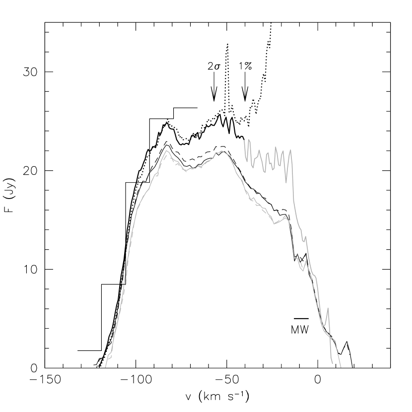
Figure 1.— NGC6822 global Hi profiles. The thick dotted line is the single-dish profile not corrected for Galactic emission. The thick drawn line is the same profile correced for Galactic emission. The black part of the profile indicates the velocity range unaffected by Galactic foreground emission, the grey part indicates the velocity range where the corrections are significant. The horizontal line marked ‘MW’ indicates the velocity range where in the single-dish data the signal from NGC 6822 could not be distinghuished from Galactic emission. The single-dish profiles in this velocity range were interpolated (see text). The thin curves are the global profiles as derived from atca data. The black full curve represents the B96 data, black dashed is the B48 data; the grey full curve is the B24 data; the grey dashed curve represents the B12 data. The histogram in the velocity range $-130\ \,\mbox{km}\,\mbox{s}^{-1}<V<-60\ \,\mbox{km}\,\mbox{s}^{-1}$ is the unaffected part of the HIPASS global profile with a velocity resolution of 13.2 $\,\mbox{km}\,\mbox{s}^{-1}$. Arrows in the plot indicate the velocities where the Galactic emission has fallen to 1 per cent of its peak value of $\sim 50$ Jy beam^-1, and where the level of Galactic emission equals twice the noise in the single-dish data cube.

Figure 2.— Channel maps of the B12 data cube. Velocities are indicated in the top-left corners of each sub-panel. The grayscales run from 0 mJy beam^-1 (white) to 90 mJy beam^-1 (black). Contours in the top-left channel indicate (from the inside out) where the sensitivity has dropped to 90, 80 and 60 per cent of the central value. The channel spacing is 1.6 $\,\mbox{km}\,\mbox{s}^{-1}$, only every second channel is shown.

Figure 2.— Continued — As in previous panel. Contours in the bottom-right channel indicate (from the inside out) where the sensitivity has dropped to 90, 80 and 60 per cent of the central value. Note the different field centre compared to the previous panel. Also note the Galactic contamination in the $-11.2$ and $-8.0$ $\,\mbox{km}\,\mbox{s}^{-1}$ channels.

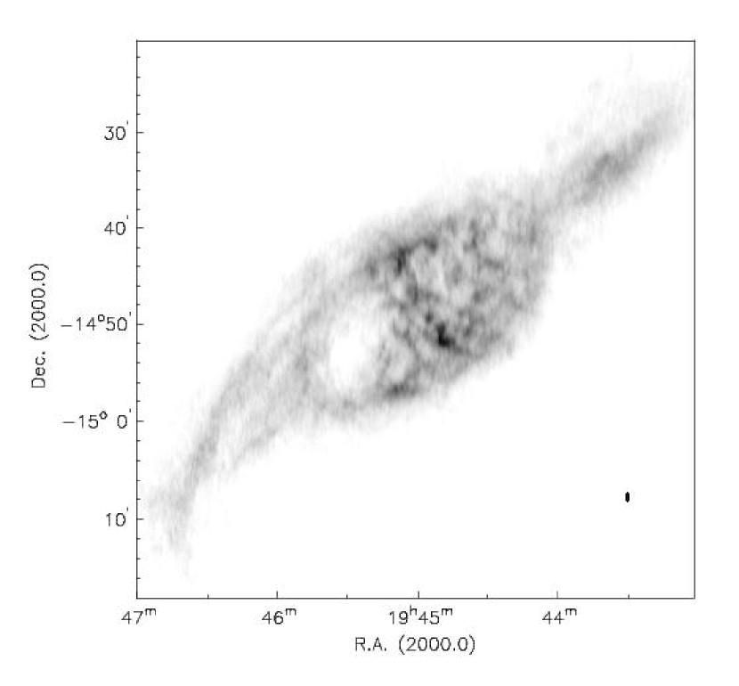
Figure 4.— Integrated Hi column density or zeroth moment map. The grayscale levels run from $1\cdot 10^{20}$ cm^-2 (white) to $4.3\cdot 10^{21}$ cm^-2 (black), which is also the maximum column density occuring in this map. The beam of $42.4^{\prime\prime}\times 12.0^{\prime\prime}$ is indicated in the bottom-right corner. See Weldrake et al. (2003) for additional representations of this column density map.

Figure 5.— Azimuthally averaged Hi profile. The $4\sigma$ level in a single channel map is indicated as well as the column value of $5\cdot 10^{20}$ cm^-2 (not corrected for inclination) that we use to indicate the edge of the Hi disk. Note that this occurs well above the sensitivity limit of the data.

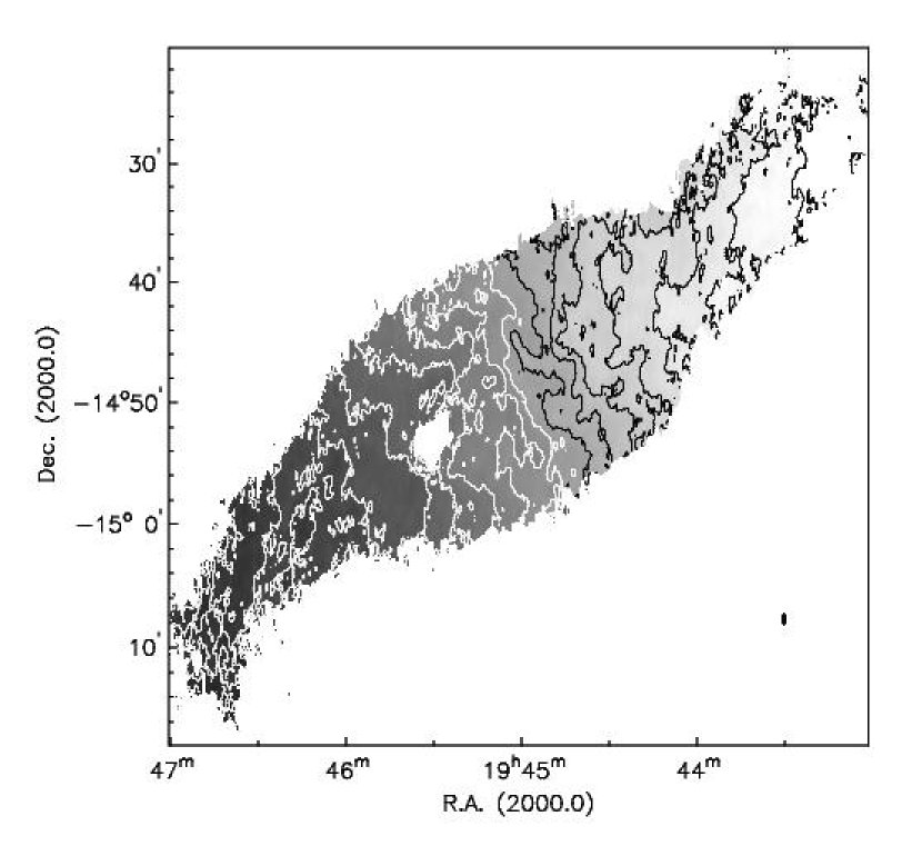
Figure 6.— Velocity field or first moment map. The black contours run from a central value of $-58$ $\,\mbox{km}\,\mbox{s}^{-1}$ to $-100$ $\,\mbox{km}\,\mbox{s}^{-1}$ in the NW, decreasing in steps of 7 $\,\mbox{km}\,\mbox{s}^{-1}$. The white contours run from a central value of $-51$ $\,\mbox{km}\,\mbox{s}^{-1}$ to a value of $+12$ $\,\mbox{km}\,\mbox{s}^{-1}$ in the SE, increasing in steps of 7 $\,\mbox{km}\,\mbox{s}^{-1}$.

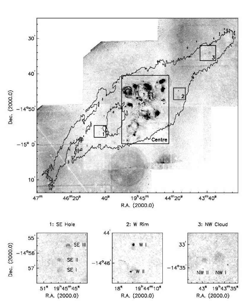
Figure 7.— The H$\alpha$ distribution in NGC6822. The top panel shows the entire extent of our H$\alpha$ data. The contour indicates the edge of the Hi disk at $5\cdot 10^{20}$ cm^-2 (not corrected for inclination). The large box labeled “Centre” marks the central area shown in more detail in Fig. 8. The boxes labeled “1”, “2” and “3” show the outlying areas where new HII regions were found. These areas are shown in more details in the small panels at the bottom.

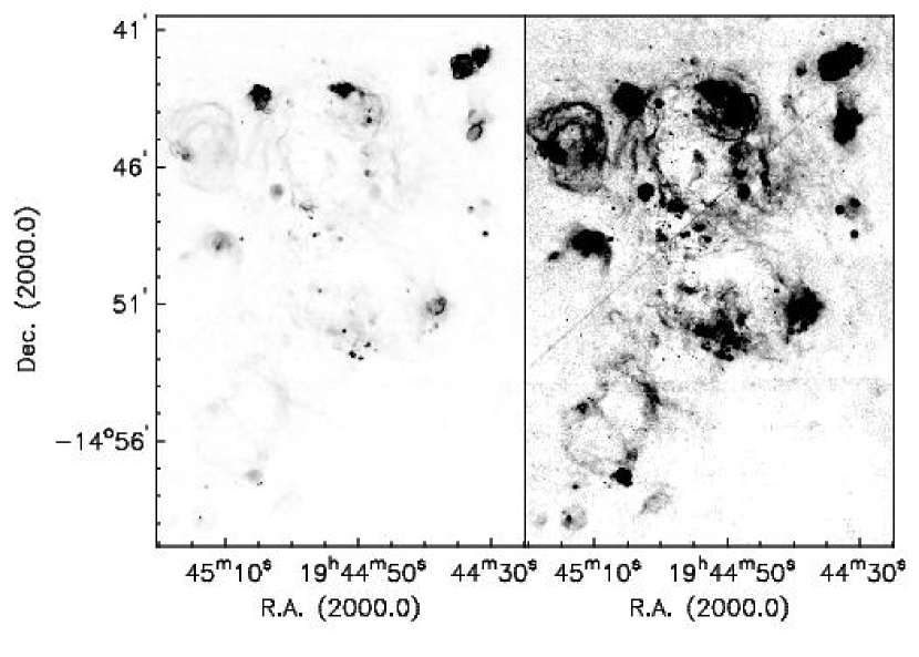
Figure 8.— The H$\alpha$ distribution in the central part of NGC6822 as indicated in Fig. 7. The left panel shows a low-contrast image of the H$\alpha$ distribution, clearly showing the population of bright H$\alpha$ regions, as well as the compact, high surface brightness regions. The right panel shows a high-contrast image of the same field emphasizing the network of low-surface brightness H$\alpha$ filaments found throughout the central part of NGC 6822.

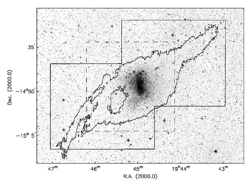
Figure 9.— The areas covered by both sets of Suprimecam observations overlaid on a DSS image of the field around NGC 6822. The large full box shows the field covered by the deep survey. The smaller dashed box shows the field of the shallow survey. The merged catalog covers the overlap between both sets. The contour indicates the edge of the Hi disk at $5\cdot 10^{20}$ cm^-2 (not corrected for inclination).

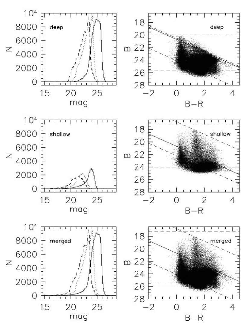
Figure 10.— Magnitude distributions and CMDs based on the two Subaru data sets. Top row: The deep catalogue. Note that we only show the data from the overlap area with the shallow survey. Middle row: The shallow catalogue. Bottom row: The merged catalogue. The left panels show the magnitude distributions in the three catalogues. The full histograms shows the $B$-band data, the dotted histograms the $R$-band and the dashed histograms the $I$-band data. The right panels show the $B$ vs $B-R$ CMDs for the three catalogues. The horizontal dashed lines show the completeness limits in $B$, the diagonal dashed lines the limits in $R$. For the deep survey (top) these limits occur at $m_{B}=(20.0,25.6)$ and $m_{R}=(20.5,24.1)$. The shallow survey limits (middle) occur at $m_{B}=(17.3,24.1)$ and $m_{R}=(16.8,22.2)$. The limits for the merged catalogue (bottom) are the extremes of these limits. The full diagonal line at $m_{R}=20.7$ indicates the magnitude cut applied to merge the shallow and deep catalogues. See text for more details.

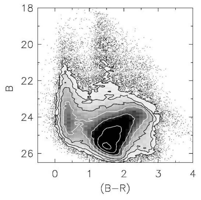
Figure 11.— Density contours of the CMD diagram of the merged catalogue. The CMD was binned in intervals of $0.1\times 0.1$ mag. Contour levels are 20, 40, 80, 160, 320, 640, 1280 stars per bin. For CMD surface densities less than 20 stars the individual stars are plotted.

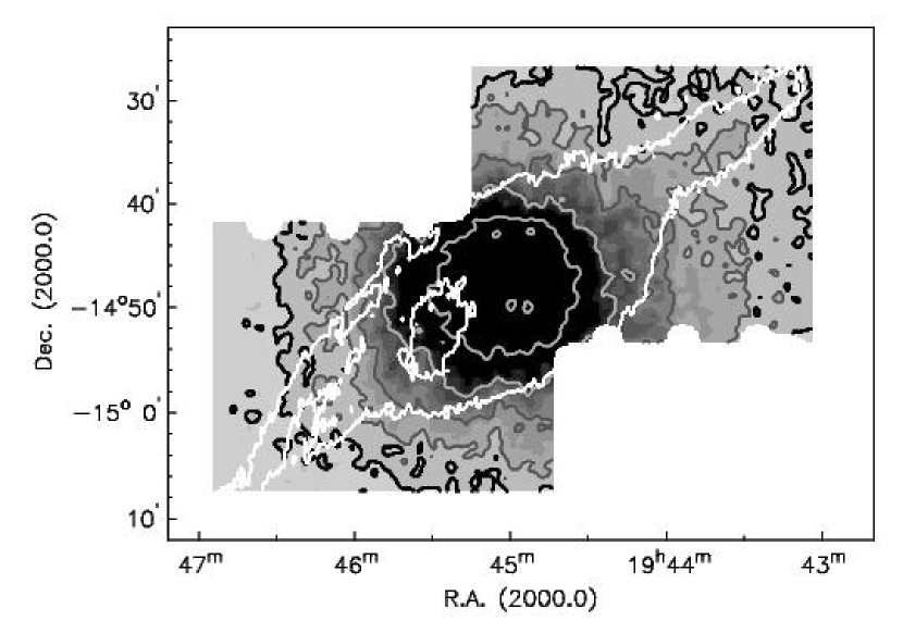
Figure 12.— Stellar surface density distribution based on the deep catalog. Surface densities shown here were derived by counting stars in $12^{\prime\prime}\times 12^{\prime\prime}$ boxes, smoothing the resulting distribution to $48^{\prime\prime}$. The thick black contour represents a smoothed surface density of 1.1. We take surface densities lower than this number to describe the field environment. The grey contours show the 2, 4, 8, 16 and 32 surface density levels. The white contour indicates the edge of the Hi disk at $5\cdot 10^{20}$ cm^-2 (not corrected for inclination). Note that NGC 6822 is much more extended to the NW as it is to the SE. The white features along the edges of the field are artefacts of the binning and smoothing procedures used.

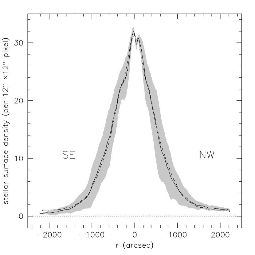
Figure 13.— Azimuthally averaged stellar surface density distribution as derived from Fig. 12. The tilted ring parameters as described in Sec. 2.5 were used. The dashed line represents the surface density averaged over both sides of the galaxy. The full lines represent the profiles of the NW (approaching) and SE (receding) side, as indicated in the plot. The grey areas indicate the 1$\sigma$ variation in the stellar surface density in each annulus.

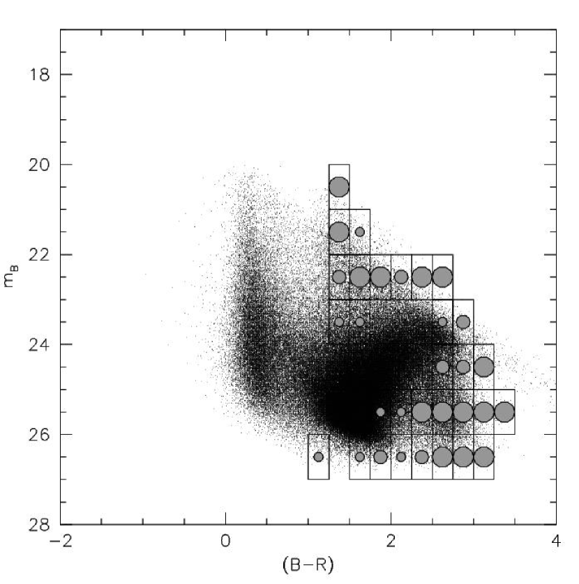
Figure 14.— CMD of the deep catalogue with degree of field contamination overplotted. Stars were counted in each CMD bin (as indicated in Figure), and compared after scaling (see text). The largest symbols indicate a field star density between 0.5 and 2.0 times the galaxy star density, that is, the regions dominated by field stars. Intermediate symbols indicate a field fraction between 0.25 and 0.5. The smallest symbols indicate a field fraction between 0.25 and 0.15. Areas without symbols have a field fraction less than 0.15, and can be considered to be uncontaminated by field stars.

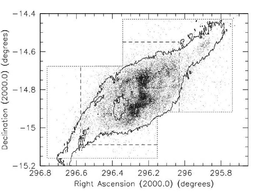
Figure 15.— Distribution of blue stars on the sky. Areas covered by the deep (short dashed box) and shallow (long dashed box) are indicated. Inside the area of the shallow catalogue we plot the blue stars from the merged catalogue. The contour indicates the edge of the Hi disk at $5\cdot 10^{20}$ cm^-2 (not corrected for inclination).

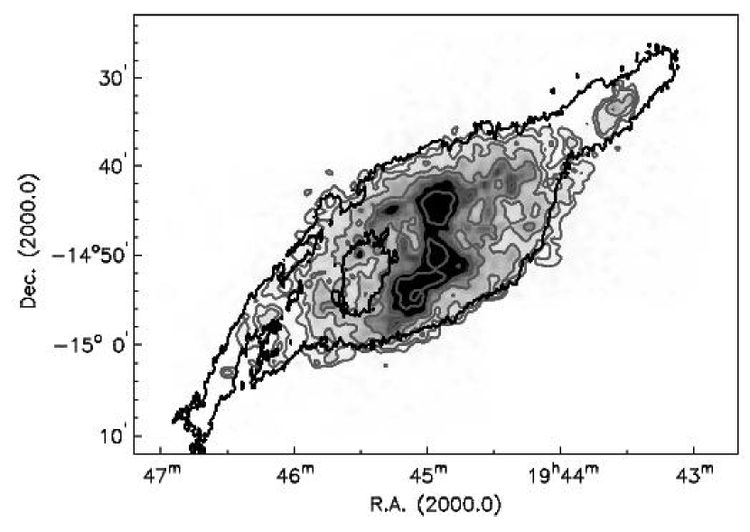
Figure 16.— Number density of blue stars measured in $12^{\prime\prime}\times 12^{\prime\prime}$ boxes, smoothed to a final resolution of $48^{\prime\prime}\times 48^{\prime\prime}$. The grayscale levels run from 0 to 5 stars per smoothed $12^{\prime\prime}$ pixel. The contour levels indicate 0.25, 0.5, 1, 2, 4 and 8 stars per pixel. The contour indicates the edge of the Hi disk at $5\cdot 10^{20}$ cm^-2 (not corrected for inclination).

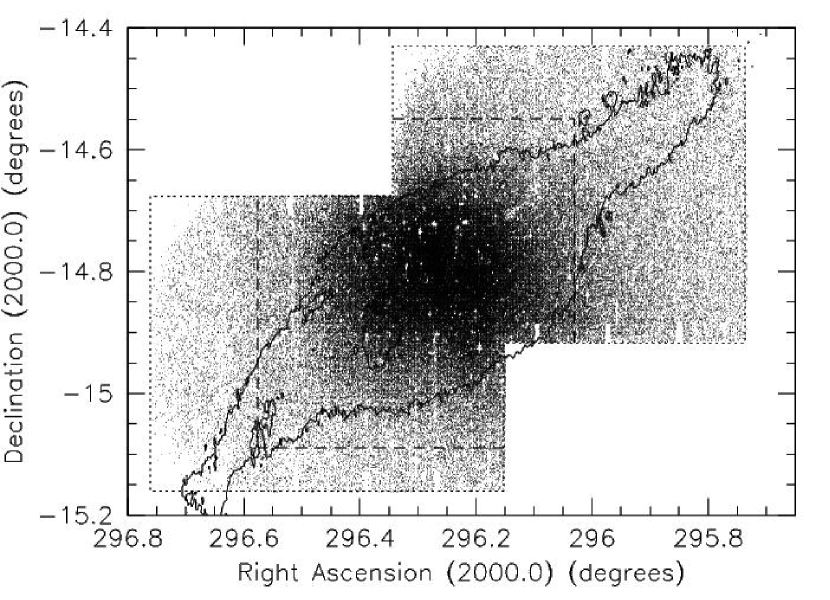
Figure 17.— Distribution of the old population on the sky. Only stars in field uncontaminated areas of the CMD are plotted. The contour indicates the edge of the Hi disk at $5\cdot 10^{20}$ cm^-2 (not corrected for inclination).

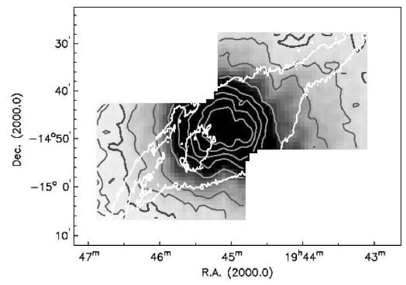
Figure 18.— Surface density of the old population measured in $12^{\prime\prime}\times 12^{\prime\prime}$ boxes, smoothed to a final resolution of $48^{\prime\prime}\times 48^{\prime\prime}$. Greyscale levels run from densities of 0 to 100. Contours with levels 2, 4, 8 (thick contour), 16, 32, followed by levels from 80 to 280 in steps of 50. The white contour indicates the edge of the Hi disk at $5\cdot 10^{20}$ cm^-2 (not corrected for inclination).

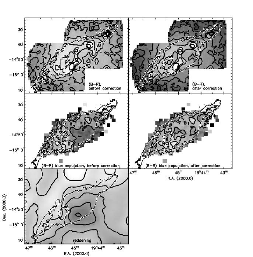
Figure 19.— Colour of the stellar disk. The top-left panel shows the colours of the field-uncontaminated disk population. The lowest (bluest) contour is $B-R=1.3$. Contours increase in steps of 0.1 from white to dark-gray. The top-right panel shows the same population but after correction for foreground reddening, as shown in the bottom-left panel. The lowest contour is $B-R=0.85$, and contours increase in steps of 0.15 from white to dark-gray. The centre-left panel shows the colours of the field-uncontaminated blue star population only. Contours run from $B-R=0.3$ (white) to 0.55 (dark-gray), in steps of 0.05. The long contour running over the centre of the galaxy has value $B-R=0.45$. The centre-right panel shows the same population but after correction for foreground reddening, as shown in the bottom-left panel. The lowest contour is $B-R=-0.05$, increasing in steps of 0.05 from white to dark-gray. The bottom-left panel shows the reddening values from the Schlegel et al. (1998) maps. Contours run from $E(B-V)=0.18$ (white) to 0.26 (dark-gray) in steps of 0.02. The thin white-black contour indicates the edge of the Hi disk at $5\cdot 10^{20}$ cm^-2 (not corrected for inclination).

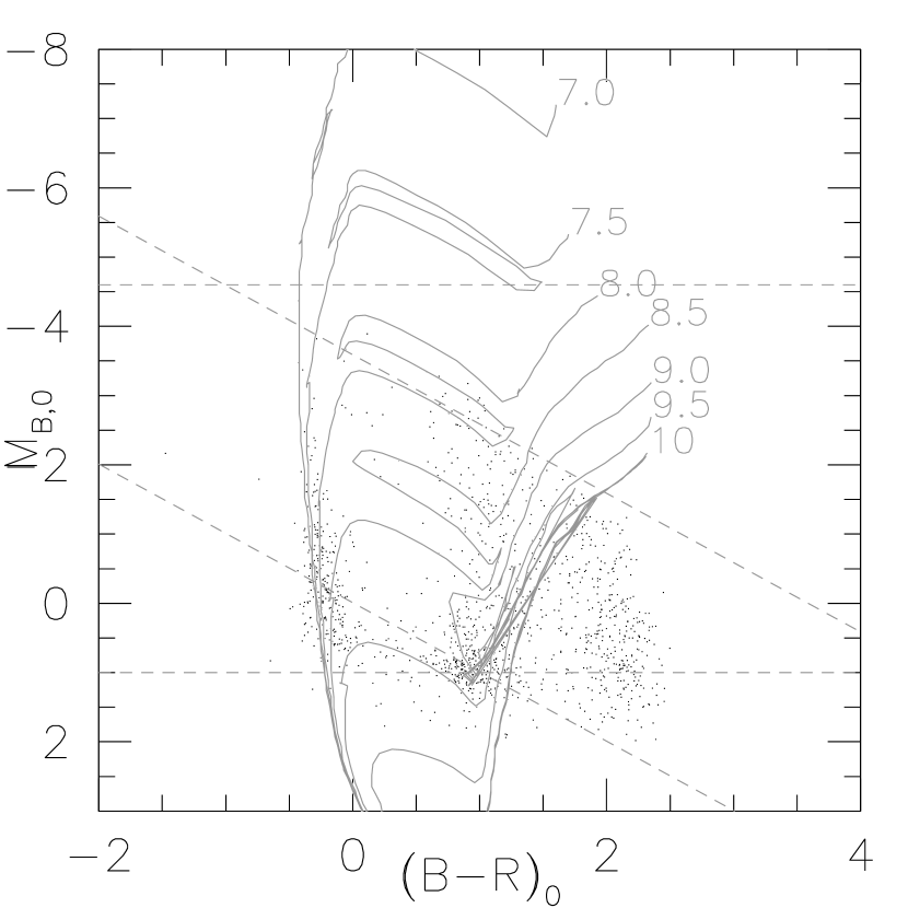
Figure 20.— CMD of the NW cloud. Several $Z=0.004$ isochrones from Girardi et al. (2000) are superimposed. The log(age) is indicated next to each isochrone. The dashed lines indicate saturation and completeness limits of the deep catalogue as indicated in Fig. 10.

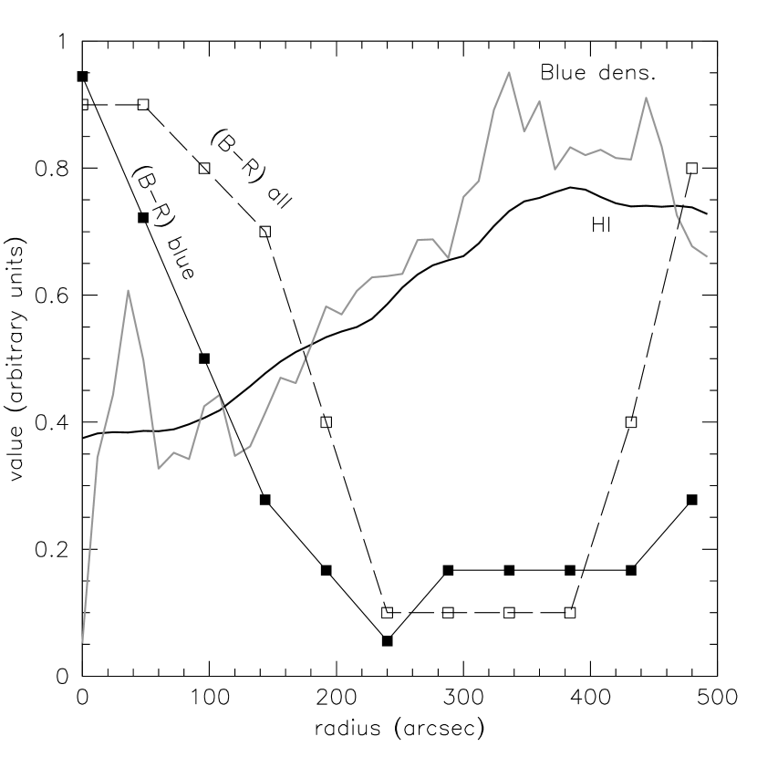
Figure 21.— Radial profiles with respect to the centre of the SGS. Shown are the Hi distribution (thick full line) and the density of blue stars (thick grey line). Also shown are the colour of the blue stars (full line with filled squares) and the colour of the total population (dashed line with open squares). The units along the vertical axis are arbitrary.

Figure 22.— Outline of the SGS superimposed on various mass component distributions. The inner thick ellipse has a semi-major axis of 250^′′. The outer thick ellipse has a semi-major axis of 430^′′. The thin dashed ellipses have semi-major axes of $170^{\prime\prime}$ and $300^{\prime\prime}$. For description see text. Shown in the top-left panel is the distribution of Hi . Top-right shows the H$\alpha$, bottom-left the distribution of blue stars, bottom right the $B-R$ colour of the blue population (dark corresponds with a red colour, light with a blue colour).

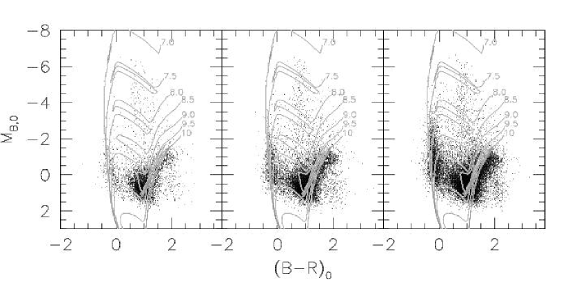
Figure 23.— CM diagrams of annuli in the SGS. Left panel shows the CMD of the star within the $170^{\prime\prime}$ semi-major axis ellipse shown in the previous figure. The central panels shows stars between semi-major axes $170^{\prime\prime}$ and $300^{\prime\prime}$. The right panel shows the stars in the annulus with semi-major axes between $300^{\prime\prime}$ and $430^{\prime\prime}$.

References

- Barnard (1884) Barnard, E.E., 1884, Sidereal Messenger, 3, 254
- Barnes et al. (2001) Barnes, D. G., et al. 2001, MNRAS, 322, 486
- Battinelli et al. (2003) Battinelli, P., Demers, S., & Letarte, B. 2003, A&A, 405, 563
- Braun et al. (1997) Braun, J. M., Bomans, D. J., Will, J., & de Boer, K. S. 1997, A&A, 328, 167
- Chyży et al. (2003) Chyży, K. T., Knapik, J., Bomans, D. J., Klein, U., Beck, R., Soida, M., & Urbanik, M. 2003, A&A, 405, 513
- de Blok & Walter (2000) de Blok, W. J. G. & Walter, F. 2000, ApJ, 537, L95
- de Blok & Walter (2003) de Blok, W. J. G. & Walter, F. 2003, MNRAS, 341, L39
- Efremov et al. (1999) Efremov, Y. N., Ehlerová, S., & Palouš , J. 1999, A&A, 350, 457
- Ekers & Rots (1979) Ekers, R. D., & Rots, A. H. 1979, ASSL Vol. 76: IAU Colloq. 49: Image Formation from Coherence Functions in Astronomy, 61
- Ferguson et al. (1998) Ferguson, A. M. N., Wyse, R. F. G., Gallagher, J. S., & Hunter, D. A. 1998, ApJ, 506, L19
- Gallart et al. (1996a) Gallart, C., Aparicio, A., Bertelli, G., & Chiosi, C. 1996, AJ, 112, 2596
- Gallart et al. (1996b) Gallart, C., Aparicio, A., Bertelli, G., & Chiosi, C. 1996, AJ, 112, 1950
- Gallart et al. (1996c) Gallart, C., Aparicio, A., & Vilchez, J. M. 1996, AJ, 112, 1928
- Gerritsen & Icke (1997) Gerritsen, J. P. E., & Icke, V. 1997, A&A, 325, 972
- Girardi et al. (2000) Girardi, L., Bressan, A., Bertelli, G., Chiosi, C. 2000, A&AS, 141, 371
- Haynes et al. (1998) Haynes, R., Staveley-Smith, L., Mebold, U., Kalberla, P., White, G., Jones, P., Dickey, J., Green, A. 1998, IAU Symp. 190, 63
- Hodge (1980) Hodge, P.W., 1980, ApJ, 241, 125
- Hodge et al. (1988) Hodge, P., Lee, M. G., & Kennicutt, R. C. 1988, PASP, 100, 917
- Hodge et al. (1989) Hodge, P., Lee, M. G., & Kennicutt, R. C. 1989, PASP, 101, 32
- Hodge et al. (1991) Hodge, P., Smith, T., Eskridge, P., MacGillivray, H., Beard, S. 1991, ApJ, 379, 621
- Hubble (1925) Hubble, E., 1925, ApJ, 62, 409
- Israel et al. (1996) Israel, F.P., Bontekoe, Tj.R., Kester, D.J.M, 1996, A&A, 308, 723
- Jorsater & van Moorsel (1995) Jorsater, S., & van Moorsel, G. A. 1995, AJ, 110, 2037
- Kamphuis et al. (1991) Kamphuis, J., Sancisi, R., & van der Hulst, T. 1991, A&A, 244, L29
- Kim et al. (2003) Kim, S., Staveley-Smith, L., Dopita, M. A., Sault, R. J., Freeman, K. C., Lee, Y., & Chu, Y. 2003, ApJS, 148, 473
- Komiyama et al. (2003) Komiyama, Y., et al. 2003, ApJ, 590, L17
- Letarte et al. (2002) Letarte, B., Demers, S., Battinelli, P., & Kunkel, W. E. 2002, AJ, 123, 832
- Loeb & Perna (1998) Loeb, A., & Perna, R. 1998, ApJ, 503, L35
- Massey et al. (1995) Massey, P., Armandroff, T. E., Pyke, R., Patel, K., & Wilson, C. D. 1995, AJ, 110, 2715
- Massey et al. (2000) Massey, P., Hodge, P. W., Jacoby, G. H., King, N. L., Olson, K. A. G., Saha, A., & Smith, C. 2000, BAAS, 32, 1595
- Mateo (1998) Mateo, M.L. 1998, ARA&A, 36, 435
- Miyazaki et al. (2002) Miyazaki, S., et al. 2002, PASJ, 54, 833
- Ott et al. (2001) Ott, J., Walter, F., Brinks, E., Van Dyk, S. D., Dirsch, B., & Klein, U. 2001, AJ, 122, 3070
- Perrine (1922) Perrine, C.D., 1922, MNRAS, 82, 489
- Puche et al. (1992) Puche, D., Westpfahl, D., Brinks, E., & Roy, J. 1992, AJ, 103, 1841
- Rhode et al. (1999) Rhode, K. L., Salzer, J. J., Westpfahl, D. J., & Radice, L. A. 1999, AJ, 118, 323
- Schlegel et al. (1998) Schlegel, D. J., Finkbeiner, D. P., & Davis, M. 1998, ApJ, 500, 525
- Skillman et al. (1989) Skillman, E.D., Terlevich, R., Melnick, J. 1989, MNRAS, 240, 563
- Staveley-Smith et al. (1996) Staveley-Smith, L., , Wilson, W.E., Bird, T.S., Disney, M.J., Ekers, R.D., Freeman, K.C., Haynes, R.F., Sinclair, M.W., Vaile, R.A., Webster, R.L., Wright, A.E., 1996, PASA, 13, 243
- Staveley-Smith et al. (1997) Staveley-Smith, L., Sault, R. J., Hatzidimitriou, D., Kesteven, M. J., & McConnell, D. 1997, MNRAS, 289, 225
- Stewart & Walter (2000) Stewart, S. G., & Walter, F. 2000, AJ, 120, 1794
- Tenorio-Tagle & Bodenheimer (1988) Tenorio-Tagle, G., & Bodenheimer, P. 1988, ARA&A, 26, 145
- van den Bergh (1999) van den Bergh, S. 1999, AJ, 117, 2211
- Vorobyov & Basu (2005) Vorobyov, E. I., & Basu, S. 2005, A&A, 431, 451
- Walter & Brinks (2001) Walter, F., & Brinks, E. 2001, AJ, 121, 3026
- Walter & Brinks (1999) Walter, F., & Brinks, E. 1999, AJ, 118, 273
- Walter et al. (1998) Walter, F., Kerp, J., Duric, N., Brinks, E., & Klein, U. 1998, ApJ, 502, L143
- Weldrake et al. (2003) Weldrake, D. T. F., de Blok, W. J. G., & Walter, F. 2003, MNRAS, 340, 12
- Wyder (2003) Wyder, T.K. 2003, AJ, 125, 3097