The Dependence of Galaxy Colors on Luminosity and Environment at $z\sim 0.4$

Abstract

We analyse the $B-R_{c}$ colors of galaxies as functions of luminosity and local galaxy density using a large photometric redshift catalog based on the Red-Sequence Cluster Survey. We select two samples of galaxies with a magnitude limit of $M_{R_{c}}<-18.5$ and redshift ranges of $0.2\leq z<0.4$ and $0.4\leq z<0.6$ containing $\sim 10^{5}$ galaxies each. We model the color distributions of subsamples of galaxies and derive the red galaxy fraction and peak colors of red and blue galaxies as functions of galaxy luminosity and environment. The evolution of these relationships over the redshift range of $z$$\sim$0.5 to $z$$\sim$0.05 is analysed in combination with published results from the Sloan Digital Sky Survey. We find that there is a strong evolution in the restframe peak color of bright blue galaxies in that they become redder with decreasing redshift, while the colors of faint blue galaxies remain approximately constant. This effect supports the “downsizing” scenario of star formation in galaxies. While the general dependence of the galaxy color distributions on the environment is small, we find that the change of red galaxy fraction with epoch is a function of the local galaxy density, suggesting that the downsizing effect may operate with different timescales in regions of different galaxy densities.

1. Introduction

Many investigations in the past 30 years have shown that galaxy populations, manifested by galaxy colors, spectra, and morphological distributions, have a strong dependence on the environment and luminosity of the galaxies (e.g., Melnick & Sargent 1970; Dressler 1980; de Vaucouleurs 1961 and many other subsequent studies). More recently, much more detailed analyzes of galaxy color distributions in the local universe have become available using large galaxy samples of tens of thousands from the Sloan Digital Sky Survey (SDSS). Baldry et al. (2004) and others show that the colors of galaxies can be neatly separated into components of red and blue galaxies. Balogh et al. (2004, hereafter B04) were able to delineate the dependence of galaxy colors on galaxy luminosity and environment, concluding that there is only a weak dependence on the latter.

In this Letter we present a similar study of galaxy samples at redshift between 0.2 and 0.6 using the photometric redshift galaxy catalogs from the Red-Sequence Cluster Survey (RCS) from Hsieh et al. (2005, hereafter H05). Combined with results from a $z$$\sim$0.05 sample from the SDSS (B04), we examine the trend of the dependence of galaxy colors on luminosity and environment at different epochs. In §2 we briefly describe the photometric redshift galaxy sample and the measurement techniques. We present the results in §3; their implications are discussed and summarized in §4. We adopt a flat cosmology with $\Omega_{m}=0.3$, $\Omega_{\Lambda}=0.7$ and $H_{0}=70$ km s^-1Mpc^-1.

2. The Photometric Redshift Galaxy Data

The RCS is a 92 square degree imaging survey in the $z^{\prime}$ and $R_{c}$ bands conducted with the CFHT 3.6m and the CTIO 4m to search for galaxy clusters in the redshift range of $z<1.4$ (see Gladders & Yee 2005). Additional imaging in the $V$ and $B$ bands was also obtained for 33.6 square degrees in the northern patches using the CFH12K camera. The observation and data reduction techniques are discussed in detail in Gladders & Yee (2005) for the $z^{\prime}$ and $R_{c}$ data, and in H05 for the $V$ and $B$ data. Photometric redshifts for 1.2 million galaxies using the four-color photometry are derived using an empirical training set method with 4,924 spectroscopic redshifts. Detailed descriptions of the photometric redshift method and the precision and completeness of the sample are presented in H05.

Upper large panel: Distributions of rest $(B-R)$ colors for galaxies in subsamples of different surface density ($\Sigma_{5}$) and luminosity ($M_{R_{c}}$) for $0.2\leq z<0.4$. Subpanels for different densities are plotted horizontally, while subpanels for different absolute magnitudes are plotted vertically. Lower large panel: same for $0.4\leq z<0.6$. Solid lines are two-Gaussian fits to the distributions of blue and red galaxies.

We select samples of galaxies covering two moderate redshift intervals using conservative criteria to minimize redshift and color errors. We choose galaxies with absolute magnitudes $M_{R_{c}}<-18.5$ in the photometric redshift bins: $0.2\leq z<0.4$ (hereafter, the $z$$\sim$0.3 sample) and $0.4\leq z<0.6$ (hereafter, the $z$$\sim$0.5 sample) with redshift uncertainty $\sigma_{z}/(1+z)<0.1$, where $\sigma_{z}$ is the computed photometric redshift uncertainty (see H05). The absolute magnitudes are corrected for K-correction and estimated evolution. For each galaxy, we use model colors computed from the spectral energy distributions of galaxies from Coleman et al. (1980) to estimate a galaxy spectral type based on the observed $R_{c}-z^{\prime}$ color, and derive K-corrections for the $B$ and $R_{c}$ magnitudes. We approximate the $R_{c}$ band luminosity evolution by $M(z)=M(0)-Qz$ (see Lin et al. 1999), where we adopted $Q=1.5$ for early-type galaxies ($B-R_{c}>1.8$) and $Q=1.0$ for late-type galaxies ($B-R_{c}<1.8$). We further limit our galaxy sample to be at least 100^′′ from the edges of the fields. These criteria produce a sample of 106,095 and 124,004 galaxies for the $z$$\sim$0.3 and $z$$\sim$0.5 sample, respectively.

We estimate the local galaxy density using a projected surface density as a proxy (see, e.g., Dressler 1980). For each galaxy in the primary sample, we measure $R_{5}$, the distance to the fifth nearest neighbor with $M_{R_{c}}\leq-19.5$, from which a local surface density parameter $\Sigma_{5}$ in units of Mpc^-2 (proportional to $R_{5}^{-2}$) is computed. For counting the five objects we select only those with photometric redshifts within 2$\sigma_{z}$ of the primary galaxy. A completeness correction for each neighbor is applied, as not all galaxies within the sampling magnitude range satisfy the redshift uncertainty criterion. The completeness factor is estimated using the ratio of the total number of galaxies within a 0.1 mag bin at the magnitude of the neighbor galaxy to the number of galaxies in that bin with photometric redshifts satisfying the redshift uncertainty criterion. Since red galaxies on average have lower photometric redshift uncertainties, we refine our completeness correction by computing the factor separately for red and blue galaxies, separated at $B-R_{c}=1.8$. The average completeness correction factor is $\sim$1.10. We count the nearest neighbors to the primary galaxy by summing the corrected weight for each galaxy until the total is $\geq 5.0$.

To be able to put the $\Sigma_{5}$ parameter for galaxies at different redshift on a comparative scale, a background correction must be applied to $\Sigma_{5}$. This is estimated for each primary galaxy by computing the average number of galaxies in a circle of radius $R_{5}$ using galaxies in the same RCS patch (of size $\sim 2.5$ deg ², see Gladders & Yee 2005) that satisfy the redshift and magnitude criteria used for the counting of the neighbors. Completeness corrections are also applied in the counting of the background galaxies. The average background correction applied is 5.59 galaxies, with a scatter of 4.43. The stochastic nature of the background produces negative local densities; for convenience, we add 5 to $\Sigma_{5}$ for the purpose of displaying some of the results.

Figure 1.— Red galaxy fraction, $f_{r}$, as a function of local galaxy density for samples of different luminosities for the two redshift bins.

Figure 2.— Galaxy color ($(B-R_{c})_{0}$) peak of the blue and red galaxy distributions as a function of local galaxy density for samples of different luminosities for the two redshift bins.

3. Results

The two panels of Figure 1 show the rest $(B-R_{c})_{0}$ distributions in bins of absolute magnitude and $\Sigma_{5}$ for the $z$$\sim$0.3 and $z$$\sim$0.5 bins. We divide the galaxies into subsamples of local density such that the first bin contains the least dense 12.5% of the galaxies; the next three bins, each of the successive 25%; and the last bin, the most dense 12.5%. The solid lines are the two-Gaussian fits for the red and blue populations. Qualitatively, the two-Gaussian model that has been used for the SDSS $z\sim 0.05$ galaxy samples by Baldry et al. (2004) and B04 is also a reasonable descriptor of the data at these higher redshifts. For comparison purposes, we note that the approximate transformations between the SDSS system and our data are: $r\sim R_{c}+0.5$ and $u-r\sim 2(B-R_{c})-0.4$ (based on galaxy color data from Fukugita et al. 1995). We also repeat the calculation using a sample with a more liberal error criterion, $\sigma_{z}/(1+z)<0.4$; this produces qualitatively identical results, showing that the incompleteness correction works well.

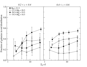
Figure 2 shows the fraction of red galaxies, $f_{r}$, derived from integrating the Gaussian fits, as a function of local density for each magnitude bin for the two redshift samples. The uncertainty for each $f_{r}$ value is estimated by generating 100 Monte-Carlo realizations based on the errors on the parameters of the corresponding two-Gaussian fit. We take the 68% confidence limits on $f_{r}$ for the 100 results to be the $\pm 1\sigma$ uncertainty. For both redshift bins, there is a strong dependence of $f_{r}$ on luminosity, covering a factor of 5–6, with the luminous galaxy samples having the higher values. Within each magnitude bin, the dependence of $f_{r}$ on local density, however, is relatively moderate, especially for the fainter galaxies.

Figure 3 illustrates the dependence of the peak $(B-R_{c})_{0}$ of the Gaussian fits on local density for galaxies of different luminosities. Similar to the SDSS result at $z$$\sim$0.05 (B04; Hogg et al. 2003), the peak colors of the color distributions of both the red and the blue galaxies have only a weak dependence on the local galaxy density. We note that because of the scatter of the background corrections, there will be some blurring of the local density parameter; however, this smoothing should have minimal effect at the high density bins, where the density is much higher than the scatter in the background correction.

4. Discussion and Conclusions

Using the three redshift epochs, we find a number of interesting evolutionary effects in the color distribution of galaxies. We find the peak colors of the red galaxy distributions to be remarkably similar over the three redshift bins. The color peaks for both the $z$$\sim$0.3 and $z$$\sim$0.5 samples for the different magnitude subsamples range from $(B-R_{c})_{0}$ of $\sim$ 1.3 to $\sim 1.6$, with the brighter red galaxies being redder. This is essentially identical to the $z$$\sim$0.05 SDSS samples of B04 over a similar luminosity range, which have $u-r\sim 2.2$ to 2.5 (or $B-R_{c}\sim 1.3$ to 1.5). Hence, there has been only minimal changes in the colors of red galaxies in all environments from $z$$\sim$0.5 to $z$$\sim$0.05. The small color changes suggest that red galaxies of all luminosities and in different environments are already well-evolved by redshift $\sim 0.6$ (e.g., see models in Bruzual & Charlot 1993).

The difference in $(B-R_{c})_{0}$ for red galaxies of different absolute magnitudes is likely due to the slope of the color-magnitude relation (CMR) for early-type galaxies. The range of $(B-R_{c})_{0}$ of $\sim$ 0.3 mag over $\sim 4.5$ mag in $M_{R_{c}}$ is equivalent to a CMR slope of $\sim$0.06, very similar to the slope of 0.03 to 0.08 found in the CMR of galaxy clusters (e.g., López-Cruz et al. 2004).

The blue galaxy color distributions, however, show a strong evolutionary effect from $z$$\sim$0.5 to $z$$\sim$0. For the $z$$\sim$0.5 sample, the peak colors of the blue galaxies are essentially independent of the luminosity of the galaxies, with values bunching up around $(B-R_{c})_{0}$ $\sim 0.85$, with a dispersion of less than 0.05 mag. Thus, on average, for all magnitudes, blue galaxies are at least as blue as the faintest blue galaxies at lower redshift. For the $z$$\sim$0.3 sample, the blue galaxies in the two brighter bins ($M_{R_{c}}<-20.5$) now have color peaks 0.2 to 0.4 mag redder than that of the faintest blue galaxy bin. Comparing to the $z$$\sim$0.05 sample of B04 (their Figure 3), the evolution is quite dramatic. Here, the peak color of each successive brighter bin shifts significantly to the red, to the point where the brightest blue galaxy bin has almost the same color peak as the faintest red galaxy bin. We also note that the bluest peaks in our data are about 0.1 mag bluer than the corresponding bin in B04.

This evolution of the blue galaxy peak colors can be interpreted in the context of a ‘down-sizing’ scenario, a term first suggested by Cowie et al. (1996). To first order, we can assume that $(B-R_{c})_{0}$ provides a measure of the specific star formation rate (SSFR, defined as the star formation rate per unit mass), or the time since the last major star formation episode (e.g., Bruzual & Charlot 1993). At $z$$\sim$0.5, blue galaxies of all luminosities have very similar $(B-R_{c})_{0}$ color peaks, which is consistent with galaxies of different masses having similar SSFRs. The mean colors of the brighter blue galaxies then become progressively redder with time, while those of the faint galaxies remain blue. This can be interpreted as the decrease in the SSFR being a strong function of the luminosity of the galaxy: the more massive the galaxy, the larger the decrease, or alternatively, the earlier in time the decrease takes place.

This interpretation is in excellent agreement with the results of Heavens et al. (2004), who analysed the $z$$\sim$0.05 SDSS spectra to recover the star formation history. Their Figure 2 shows that low-mass galaxies have a more or less constant star formation rate from $z\sim 1$, peaking at $z\sim$ 0.4 to 0.2. In comparison, the more massive galaxies have their star formation peak much earlier, and show a decline as early as $z\sim 1$, and by $z$$\sim$0.05 the SSFRs for galaxies of different masses are different by a factor of more than 10. We note the complementary nature of the techniques used to arrive at a similar conclusion, in that the Heavens et al. work is based on the reconstruction of star formation histories from present-day stellar populations, whereas our results are derived from direct measurements of galaxy colors at earlier epochs.

We find clear indications of evolution in $f_{r}$ from $z$$\sim$0.5 to $z$$\sim$0.05, in that there is a general increase in $f_{r}$ at lower redshift. Comparing our high redshift bins with the SDSS results (B04), the evolution of $f_{r}$ also appears to be a function of the local galaxy density: the $z$$\sim$0.5 sample has a much flatter dependence of $f_{r}$ on local density. In B04’s Figure 2 there is a strong local density dependence of $f_{r}$ for galaxies of all luminosities; $f_{r}$ ranges from 0.1 to 0.4 for galaxies of different luminosities in the lowest density sample, and from 0.65 to 0.85 for the highest density samples. By comparison, $f_{r}$ in our two higher redshift bins has a similar range (0.1 to 0.4) for the low density environment, but has values between 0.15 and 0.6 in the densest regions. Thus, there is a lack of faint red galaxies in the high density bins: $f_{r}<0.4$ for all but the most luminous galaxies. In other words, at $z\lower 0.43057pt\hbox{\hbox to0.0pt{\raise 2.58334pt\hbox{\hskip 1.29167pt{{$\scriptscriptstyle>$}}}\hss} \kern-1.72218pt{{$\scriptscriptstyle\sim$}}}0.2$, there are many moderately luminous to faint blue galaxies in high density regions. This drop of $f_{r}$ at high density and high redshift could be a reflection of the change in the morphology-density relation at $z\sim 0.5$ (e.g., Dressler et al. 1997; Smith et al. 2005). The lack of faint red galaxies in high density regions has also been noted by others at moderate to high redshifts (e.g., Kodama et al. 2004)

The density-dependent evolution of $f_{r}$ suggests the need for an additional element in the downsizing scenario: the downsizing timescale is a function of the environment. That is, for galaxies of similar masses, the drop in star formation rate occurs successively later for galaxies in less dense environments. The increase of the faint blue galaxy fraction in the high redshift, high density samples can be interpreted as these galaxies having their peak star formation era at a redshift of $\sim 0.3$ to 0.2 (Heavens et al. 2004), followed by a decline, resulting in a high faint red galaxy fraction at $z$$\sim$0.05 (Figure 2, B04). In the less dense regions, the star formation rate continues to be high to lower redshifts (see, e.g., Gómez et al. 2003), keeping the blue galaxy fraction high. This is supported qualitatively by the positive, if small, gradients in the $(B-R_{c})_{0}$ peak going from the least to the most dense samples, for all redshift bins.

In summary we have analysed the $(B-R_{c})_{0}$ color distribution of a sample of $\sim 230,000$ galaxies with photometric redshifts between 0.2 and 0.6 and $M_{R_{c}}<-18.5$, in combination with the results derived at $z$$\sim$0.05 by B04 using SDSS data. We find there is a strong evolution in the peak $(B-R_{c})_{0}$ colors of the blue galaxies, consistent with a downsizing star formation scenario where more massive galaxies have their peak star formation time occurring at earlier epochs. This is in excellent qualitative agreement with star formation histories of galaxies of different masses derived by Heavens et al. (2004) using the technique of “fossil stellar populations.” We also find that the evolution of the red galaxy fraction is dependent on local galaxy density, in that there is a significant deficit of faint red galaxies in rich environments at high redshift. In a future paper we will examine the evolution of the color distributions for galaxies in different local densities in various global environments (e.g., cluster core, cluster outskirt, and field), and interpret the results more quantitatively in terms of stellar mass and star formation rate via stellar population models.

References

- (1) Baldry, I.K., Glazebrook, K., Brinkmann, J., Ivezić, Z., Lupton, R.H., Nichol, R.C., & Szalay, A.S. 2004, ApJ, 600, 681
- (2) Balogh, M.L., Baldry, I.K., Nichol, R., Miller, C., Bower, R., & Glazebrook, K. 2004, ApJ, L101 (B04)
- (3) Bruzual, G. & Charlot, S. 1993, ApJ, 405, 538
- (4) Coleman, G.D., Wu, C.-C., & Weedman, D.W. 1980, ApJS, 43, 393
- (5) Cowie, L., Songila, A., Hu, E.M., & Cohen, J.G. 1996, AJ, 112, 839
- (6) de Vaucouleurs, G. 1961, ApJS, 5, 233
- (7) Dressler, A. 1980, ApJ, 236, 351
- (8) Dressler, A., et al. 1999, ApJ, 490, 577
- (9) Fukugita, M., Shimasaku, K., & Ichikawa, T. 1995, PASP, 107, 945
- (10) Gladders, M.D. & Yee, H.K.C. 2005, ApJS, 157, 1
- (11) Gómez, P.L. et al. 2003, ApJ, 584, 210
- (12) Heavens, A., Panter, Benjamin, Jeminez, R., & Dunlop, J. 2004, Nature, 428, 625
- (13) Hogg, D.W., et al. 2003, ApJ, 585, L5
- (14) Hsieh, B.C., Yee, H.K.C., Lin, H., & Gladders, M.D. 2005, ApJS, 158, 161 (H05)
- (15) Kodama, T. et al. 2004, MNRAS, 350, 1005
- (16) Lin, H., Yee, H.K.C., Carlberg, R.G., Morris, S.L., Sawicki, M., Patton, D.R., Wirth, G. & Shepherd, C.W. 1999, ApJ, 518, 533
- (17) López-Cruz, O., Barkhouse, W.A., Yee, H.K.C. 2004, ApJ, 614, 679
- (18) Melnick, J., & Sargent, W.L.W. 1977, ApJ, 215, 401
- (19) Smith, G.P., Treu, T., Ellis, R.S., Moran, S.M., & Dressler, A. 2005, ApJ, 620, 78