Measuring Fundamental Galactic Parameters with Stellar Tidal Streams and SIM PlanetQuest

Abstract

Extended halo tidal streams from disrupting Milky Way satellites offer new opportunities for gauging fundamental Galactic parameters without challenging observations of the Galactic center. In the roughly spherical Galactic potential tidal debris from a satellite system is largely confined to a single plane containing the Galactic center, so accurate distances to stars in the tidal stream can be used to gauge the Galactic center distance, $R_{0}$, given reasonable projection of the stream orbital pole on the $X_{GC}$ axis. Alternatively, a tidal stream with orbital pole near the $Y_{GC}$ axis, like the Sagittarius stream, can be used to derive the speed of the Local Standard of Rest ($\Theta_{\rm LSR}$). Modest improvements in current astrometric catalogues might allow this measurement to be made, but NASA’s Space Interferometry Mission (SIM PlanetQuest) can definitively obtain both $R_{0}$ and $\Theta_{\rm LSR}$ using tidal streams.

1. Distance to the Galactic Center

With the assumption that globular clusters trace the general shape and extent of the Milky Way (MW), Shapley (1918) first showed how they can be used to estimate the distance ($R_{0}$) to the Galactic center (GC), expected to lie at the center of the cluster distribution. Though Shapley’s first execution of this experiment exaggerated $R_{0}$ due to cluster distance scale problems, the overall scheme of mapping an extended distribution of Galactic tracer objects to determine the location of its center remains a valid, if traditionally underutilized, strategy.

The globular cluster sample is relatively small and concentrated to the GC, where dust effects introduce large distance uncertainties and a likely still incomplete and lop-sided cluster census. Population II tracers like RR Lyrae, blue horizontal branch (BHB) or giant stars are much more plentiful outside of the MW bulge. Unfortunately, the current census for these tracers is even more incomplete than for globulars. Though this situation may be remedied by currently planned wide angle surveys, several inherent problems remain with exploitation of these tracers as GC benchmarks. As with the clusters, the MW Zone of Avoidance (ZA) will always result in biased sample distributions and potential $R_{0}$ underestimates — exacerbated if surveys do not reach the far side of the MW. Even more challenging is that the global distributions of halo stars are far from dynamically mixed: Recent surveys of the above tracers reveal a halo streaked with substructure, likely originating as satellite disruption debris (e.g., Vivas et al. 2001, Newberg et al. 2002, Majewski 2004) and eroding simple halo axisymmetry.

The very existence of numerous tidal streams motivates the present contribution. Individual tidal streams actually possess a relatively simple spatial configuration. Within spherical potentials, tidal debris arms from a disrupting satellite will lie along the satellite orbital plane, which contains the GC. A sufficiently extended tidal debris arc defines that plane, which intersects the MW $X_{GC}$ axis at the GC. This simpler, almost two-dimensional geometry of tidal stream arcs removes the need for sample completeness: In principle, $R_{0}$ should be derivable from the $(l,b,$distance) distribution of only a large enough sample of tidal stream stars to define their orbital plane.

In reality, non-spherical potentials precess tidal streams. Fortunately, this is a relatively small effect in the MW, at least for $R_{GC}$’s of tens of kiloparsecs. Johnston et al. (2005; “J05”) showed the Sagittarius (Sgr) tidal stream precession is sufficiently small to conclude the MW potential is only slightly oblate within the Sgr orbit (peri:apo-Galacticon of 13:57 kpc). Moreover, as pointed out also by Helmi (2004), that part of the Sgr trailing arm arcing across the southern MW hemisphere (see Majewski et al. 2003, “MSWO”) is so dynamically young that it hasn’t had time to precess (see Fig. 5 of J05). Unfortunately, as noted by MSWO, Sgr is in almost the worst possible orientation to undertake the proposed $R_{0}$-gauging: With a virtually negligible angle between the Sgr orbital plane and $X_{GC}$ axis, small errors in the definition of the orbital plane (due to small residual precession, and the finite width of the debris plane) lead to substantial uncertainties in derivation of $R_{0}$.

The ideal tidal debris configuration for estimating $R_{0}$ has a pole closer to the $X_{GC}$ axis. Given the pace of discovery, such a stream may soon be found. Based on the nearly polar orientation of the HI Magellanic Stream and the typically measured proper motions ($\mu$’s) for the Magellanic Clouds (Gardiner & Noguchi 1996, van der Marel et al. 2002 and references therein), it is clear that a stellar counterpart to the Magellanic Stream would have almost the perfect orientation for gauging $R_{0}$.

Systematic errors in a tracer distance scale translate to estimates of $R_{0}$. However, because streams contain different stellar types (e.g., giant stars, RR Lyrae, BHB), uncertainties from photometric/spectroscopic parallaxes can be cross-checked. In most cases, reddening and crowding effects can be of negligible concern. Alternatively, with NASA’s Space Interferometry Mission (SIM), direct trigonometric parallaxes will be well within reach: For a putative Magellanic stellar stream orbiting at $\sim 50$ kpc radius, the $\sim 10$-20 $\mu$as parallaxes are well above the SIM wide-angle astrometric accuracy goal of 4$\mu$as, assuming K giant star tracers ($V\sim 18$).

As a test of what might be achieved, we ran N-body simulations of different mass satellites disrupting for 5 or 10 Gyr (whatever was needed to produce $>270^{\circ}$-long tails) in the Galactic potential that best fitted the Sgr debris stream in Law et al. (2005; “L05” hereafter). The orbit was constrained to match the current position, radial velocity (RV) and $\mu$ (Gardiner & Noguchi 1996) of the Small Magellanic Cloud (SMC), with orbital pole $(l,b)=(196,-5)^{\circ}$. All other model parameters were similar to those in L05. Each simulation was “observed” outside a $|b|>15^{\circ}$ ZA, with $\sim 10^{3}$, $10^{4}$ and $10^{5}$ tracer stars (apportioned with $\sim 90\%$ of these in the satellite core and $\sim 10\%$ in the tidal tails), and with 0, 10 and 20% random Gaussian distance errors imposed. The simplest (though not best!) analysis of these data is simply to fit a plane and measure its intersection with the $X_{GC}$ axis. With this 0th-order method, even for large samples of stars in dynamically cold streams (i.e., not that from a 10¹⁰ M_☉ progenitor) and no distance errors, relatively large ($<7\%$) systematic errors in $R_{0}$ can remain (Fig. 1) because plane-fitting does not account for the residual precessional twisting of the debris arms. The direction of precession (determined by the direction of the stream angular momentum vector) drives the sense of the imposed systemic $R_{0}$ error (i.e. closer or farther), and random distance errors add additional uncertainties depending on details of the stream orientation relative to the ZA. A better, now proven method (e.g. L05) is to use N-body modeling to reconstruct a given stellar stream; such modeling can precisely account not only for precession but also for stream dispersion and other higher order uncertainties, which would permit a more accurate identification of the center of the MW potential for an appropriately oriented stream.

Recent measurements of stellar motions around Sgr A^∗ have led to dynamical parallaxes good to 5% ($7.94\pm 0.42$ kpc; Eisenhauer et al. 2003), a measurement sure to improve with longer Sgr A^∗ field monitoring campaigns. Few percent quality trigonometric parallaxes of stars near the GC will be measured as part of a SIM Key Project. In either method, the target stars are reasonably expected to lie at the assumed center of the MW potential. The proposed use of tidal streams to measure $R_{0}$ will provide an interesting test of this hypothesis, since tidal streams orbit the true dynamical center of the integrated potential over tens of kiloparsec scales. A comparison of this center to the Sgr A^∗ distance could reveal whether the MW may be a lop-sided spiral (e.g., Baldwin et al. 1980, Richter & Sancisi 1994, Rix & Zaritsky 1995). Such lop-sidedness can, in fact, be induced by mergers of large satellites (Walker, Mihos & Hernquist 1997). In principle, three well-measured tidal streams can verify whether the GC lies along $(l,b)=(0,0)$, since the true GC should lie at a mutual intersection of the three corresponding stream orbital planes.

2. Velocity of the Local Standard of Rest

Despite decades of effort, the local MW rotation rate remains poorly known, with measurements varying by 25%. Hipparcos $\mu$’s (Feast & Whitelock, 1997) suggest that the Local Standard of Rest (LSR) velocity is $\Theta_{\rm LSR}=(217.5\pm 7.0)(R_{0}/8)$ km s^-1 — i.e. near the IAU adopted value of 220 km s^-1. But a more recent measurement of $\mu$ for Sgr A^∗ (Reid & Brunthaler 2004) yields a higher $(235.6\pm 1.2)(R_{0}/8)$ km s^-1, whereas direct HST measurements of the $\mu$’s of bulge stars against background galaxies in the same field yield $(202.4\pm 20.8)(R_{0}/8)$ km s^-1 (Kalirai et al. 2004) and $(220.8\pm 13.6)(R_{0}/8)$ km s^-1 (Bedin et al. 2003). Of course, these measures (as well as any of those depending on the Oort constants) rely on an accurate measure of $R_{0}$ (§1). The solar peculiar motion must also be known, but is a smaller correction (e.g., $5.3\pm 0.6$ km s^-1; Dehnen & Binney 1998). On the other hand, considerations of non-axisymmetry of the disk yield corrections to the measurements that suggest $\Theta_{\rm LSR}$ may be as low as $184\pm 8$ km s^-1 (Olling & Merrifield, 1998) or lower (Kuijken & Tremaine 1994). Independent methods to ascertain $\Theta_{\rm LSR}$ are of great value because it is fundamental to establishing the MW mass scale.

Eventually, as part of a Key Project of SIM, $\Theta_{\rm LSR}$ will be measured directly by the absolute $\mu$ of stars near the GC. Here we describe an independent method for ascertaining $\Theta_{\rm LSR}$ using halo tidal streams that overcomes several difficulties with working in the highly dust-obscured, crowded GC, and one also insensitive to $R_{0}$ (for all reasonable values of the latter). The ideal tidal stream for this method is one with an orbital pole lying near the $Y_{GC}$ axis. The Sgr tidal stellar stream not only fulfills this requirement, but its stars, particularly its trailing arm M giants, are ideally placed for uncrowded field astrometry at high MW latitudes, and at relatively bright magnitudes for, and requiring only the most modest precisions from, SIM. Indeed, as we show, this method is even within the grasp of future high quality, ground-based astrometric studies.

It is remarkable that the Sun presently lies within a kiloparsec of the Sgr debris plane (MSWO). The pole of the plane, $(l_{p},b_{p})=(272,-12)^{\circ}$, means that the line of nodes of its intersection with the MW plane is almost coincident with the $X_{GC}$ axis. Thus (Fig. 2) the motions of Sgr stars within this plane are almost entirely contained in their Galactic $U$ and $W$ velocity components, whereas the $V$ motions of stars in the Sgr tidal tails almost entirely reflect solar motion. To the degree that its $V$ distribution is not completely flat in Figure 2 is due to the slight amount of streaming motion projected onto the $V$ motions from the 2^∘ Sgr orbital plane tilt from $X_{GC}$, compounded by (1) Keplerian variations in the space velocity of stars as a function of orbital phase, as well as (2) precessional effects that lead to $\Lambda_{\sun}$-variable departures of Sgr debris from the nominal best fit plane to all of the debris. The latter is negligible for trailing debris but is much larger for the leading debris, which is on average closer to the GC and dynamically older compared to the trailing debris when viewed near the Galactic poles (J05). In addition, because the leading debris gets arbitrarily close to the Sun (L05), projection effects make it more complicated to use for the present purposes. Additional problems with the leading arm debris, which suggest that more complicated effects have perturbed it are discussed in L05 and J05. In contrast, the Sgr trailing tail is beautifully positioned fairly equidistantly from us for a substantial fraction of its stretch across the Southern MW hemisphere (MSWO). This band of stars arcing almost directly “beneath” us within the $X_{GC}$-$Z_{GC}$ plane provides a remarkable zero-point reference against which to make direct measurement of the solar motion almost completely independent of the Sun’s distance from the GC. The extensive mapping (MSWO) of the Sgr tails with Two Micron All-Sky Survey (2MASS) M giants provides an ideal source list for individual stellar targets from this $>360^{\circ}$-wrapped, MW polar ring.

L05 used M giant spatial (MSWO) and RV data (Majewski et al. 2004) to constrain models of Sgr disruption, best fitting when a 3.5 $\times 10^{8}$ M_☉ Sgr of 328 km s^-1 space velocity orbits with period 0.85 Gyr and apo:peri-Galactica of 57:13 kpc. These models fit what appears to be $\sim$2.5 orbits (2.0 Gyr) of Sgr mass loss in M giants. The adopted MW potential is smooth, static and given by the sum of a disk, spheroid and halo described by the axisymmetric function $\Phi_{\rm halo}=v_{\rm halo}^{2}\ln(R^{2}+[z/q]^{2}+d^{2})$ where $q$ is the halo flattening, $R$ and $z$ are cylindrical coordinates and $d$ is a softening parameter. Additional model details are given in L05.

Model fits to the Sgr spatial and velocity data allow predictions of the 6-D phase space configuration of Sgr debris. Figure 2 shows predicted $U,V,W$ velocity components of debris as a function of longitude, $\Lambda_{\sun}$, in the Sgr orbital plane (see MSWO). The debris is shown assuming $q=0.9$, $R_{0}=7$ kpc, and a characterization of the total potential whereby the LSR speed is $\Theta_{\rm LSR}$ = 220 km s^-1. L05 explores how variations in $q$ affect primarily the $U$ and $W$ (through projection along RV). Figure 3 (green, yellow, and magenta points) shows how variations in the scale of the potential, expressed through variations in adopted $\Theta_{\rm LSR}$, affect $V$. Clearly, $\Theta_{\rm LSR}$ ranging from 180 to 260 km s^-1 translates to obvious variations in observed $V$ for trailing arm stars. This effect is easily separable from any residual uncertainty in the shape of the potential or $R_{0}$: Figure 3 (red and blue points respectively) illustrates negligible $V$ changes produced by holding $\Theta_{\rm LSR}$ fixed at 220 km s^-1 but varying $q$ from 0.9 to 1.25 (i.e. oblate to prolate) and $R_{0}$ from 7 to 9 kpc.

Figure 3 is the basis for the proposed use of Sgr to measure $\Theta_{\rm LSR}$. Ideally, to execute the experiment requires obtaining $V$ from the observed $\mu$ and RVs of Sgr arm stars. However, because of the particular configuration of Sgr trailing arm debris, almost all of $V$ is reflected in the $\mu$ of these stars, and, more specifically, the reflex solar motion is contained almost entirely in the $\mu_{l}\cos(b)$ component of $\mu$ for Sgr trailing arm stars away from the MW pole. Working in the observational, $\mu$ regime means that vagaries in the derivation of individual star distances can be removed from the problem, as long as the system is modeled with a proper mean distance for the Sgr stream as a function of $\Lambda_{\sun}$. Figure 4 shows three general regimes of the trailing arm $\mu_{l}\cos(b)$ trend: (1) $\Lambda_{\sun}\gtrsim 100^{\circ}$ where $\mu_{l}\cos(b)$ is positive and roughly constant, (2) the region from $100^{\circ}\gtrsim\Lambda_{\sun}\gtrsim 60^{\circ}$ where $\mu_{l}\cos(b)$ flips sign as the debris passes through the South Galactic Pole to shift the Galactic longitudes of the trailing arm by $\sim 180^{\circ}$, and (3) $\Lambda_{\sun}\lesssim 60^{\circ}$, where $\mu_{l}\cos(b)$is negative and becomes smaller with decreasing $\Lambda_{\sun}$ (because the Sgr stream becomes increasingly farther). The sign flip in $\mu_{l}\cos(b)$ is a useful happenstance in the case where one has $\mu$ data not tied to an absolute reference frame but which is at least robust to systematic zonal errors: In this case the peak to peak amplitude of $\mu_{l}\cos(b)$ for the trailing arm stars yields (two times) the reflex motion of the Sun.

The intrinsic RV dispersion of the Sgr trailing arm has been measured to be $\sim$10 km s^-1 (Majewski et al. 2004); assuming symmetry in the two transverse dimensions of the stream gives an intrinsic $\mu$ dispersion of the Sgr trailing arm of $\sim$0.1 mas yr^-1 (see Fig. 4a). Thus, until SIM-quality proper motions exist, the measurement of the reflex solar motion by this method will be dominated by the error in $\mu$. To quantify the accuracy of the proposed method, we introduce artificial random errors into the proper motions of the five models shown in Figure 3 and calculate the accuracy with which we expect to recover the solar reflex motion.

Simply applying the formalism described above, we recover $\Theta_{\rm LSR}$ values of 212, 255, and 279 km s^-1 in models for which input $\Theta_{\rm LSR}=180,220,$ and 260 km s^-1 respectively. This indicates that the method systematically overpredicts $\Theta_{\rm LSR}$ by about 30 km s^-1; this is because (see Fig. 3) the trend of $V$ with $\Lambda_{\odot}$ is not perfectly flat but changes by $\sim 30$ km s^-1 between the peaks at $\Lambda_{\odot}=60-65^{\circ}$ and 115-120^∘. Correcting for this systematic bias, we perform 1000 tests where we randomly draw particles from the model debris streams in these ranges with artificially added random scatter in the $\mu$, and find that recovering the solar velocity to within 10 km s^-1 requires a sample of approximately 200 stars with $\mu$ measured to about 1 mas yr^-1 precision with no zonal systematics. Using the models with $\Theta_{\rm LSR}=$ 180/220/260 km s^-1, these tests recover mean values of 182/225/249 km s^-1 respectively with a dispersion of results between the tests of 10 km s^-1. As expected from Figure 3, varying $q$ and $R_{0}$ has negligible effect: Tests on models in both of these MW potentials (where $\Theta_{\rm LSR}=220$ km s^-1) recover mean values of 225 and 228 km s^-1.

Present astrometric catalogs are just short of being able to do this experiment: Hipparcos is not deep enough, the Southern Proper Motion Survey (Girard et al. 2004) has not yet covered enough appropriate sky area, and UCAC2 (Zacharias et al. 2004) has several times larger random errors than useful as well as comparably-sized zonal systematic errors at relevant magnitudes (N. Zacharias, private communication). However, to demonstrate how only modest advances in all-sky $\mu$ precisions are needed to make a definitive measurement, Figure 4 includes a direct comparison of the $\mu_{l}\cos(b)$ trend for Sgr M giants using UCAC2 $\mu$’s for 2MASS M giants. Impressively, the overall expected $\mu_{l}\cos(b)$ trends can be seen, but the large scatter and systematic shifts in the trailing arm motions belie the limits of UCAC2 accuracies at $V\sim 15$. Even a factor of two improvement in UCAC2 random errors and elimination of zonal errors might lead to a useful measurement of $\Theta_{\rm LSR}$. It is not unreasonable to expect advances in all-sky $\mu$ catalogues at this level soon (e.g., from the Origins Billion Star Survey or Gaia), but in any case SIM PlanetQuest will easily obtain the necessary $\mu$ (and parallaxes) of selected Sgr trailing arm giants.

Figure 1.— Results of plane-fitting to simulations of disrupting satellites of different masses orbiting similarly to the Magellanic Clouds. Filled, half-filled and open symbols are for simulations with no, 10% and 20% distance errors imposed on the member stars.

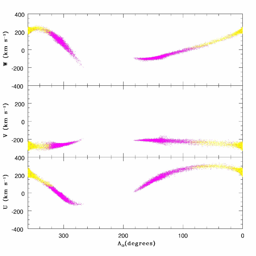
Figure 2.— Predicted $U,V,W$ velocities (right-handed system) as a function of longitude in the Sgr orbital plane ($\Lambda_{\sun}=0^{\circ}$ at present Sgr position). Debris lost on last half (yellow) and previous full (magenta) orbits are shown (see Law et al. 2005). Trailing debris stretches from $\Lambda_{\sun}=0^{\circ}$ to $\sim 180^{\circ}$; leading arm debris goes from $\Lambda_{\sun}=0^{\circ}$ to $\sim 270^{\circ}$. The Galactic model has a $q=0.9$ halo with $\Theta_{\rm LSR}=$ 220 km s^-1 and $R_{0}=$ 7 kpc.

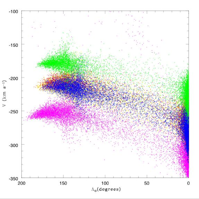
Figure 3.— Variation of the Sgr trailing arm $V$ velocities for a range of $\Theta_{\rm LSR}$, $R_{0}$, and $q$. Green, yellow, and magenta points represent debris from satellites disrupting in potentials where $q=0.9$ and $R_{0}=$ 7 kpc, but $\Theta_{\rm LSR}$ is 180, 220, and 260 km s^-1, respectively. Red and blue points represent satellite debris in potentials where $\Theta_{\rm LSR}=$ 220 km s^-1 but $q=1.25$ ($R_{0}$ fixed at 7 kpc) and $R_{0}=9$ kpc ($q$ fixed at 0.9), respectively. Note how changes in the shape of the potential have little to no effect on $V$, while changes in the scale of the potential produce large, approximately linear shifts.

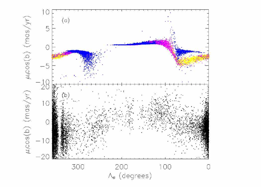
Figure 4.— (a) Same as Fig. 2 (i.e.,same MW model), but for predicted $\mu_{l}\cos(b)$ and for 2.5 orbits of mass loss. (b) Observed UCAC2 $\mu_{l}\cos(b)$ for 2MASS M giants in Galactic regions dominated by Sgr stream stars (all M giants within 7 kpc of the nominal Sgr plane and having heliocentric distances of 15-30 kpc). Note the differing vertical scales of the two panels.

References

- Baldwin et al. (1980) Baldwin, J. E., Lynden-Bell, D., & Sancisi, R. 1980, MNRAS, 193, 313
- Bedin et al. (2003) Bedin, L. R., Piotto, G., King, I. R., & Anderson, J. 2003, AJ, 126, 247
- Dehnen & Binney (1998) Dehnen, W., & Binney, J. J. 1998, MNRAS, 298, 387
- Eisenhauer et al. (2003) Eisenhauer, F., Schödel, R., Genzel, R., Ott, T., Tecza, M., Abuter, R., Eckart, A., & Alexander, T. 2003, ApJ, 597, L121
- Feast & Whitelock (1997) Feast, M. W. & Whitelock, P. 1997, MNRAS, 291, 683
- Gardiner & Noguchi (1996) Gardiner, L. T., & Noguchi, M. 1996, MNRAS, 278, 191
- Girard et al. (2004) Girard, T. M., Dinescu, D. I., van Altena, W. F., Platais, I., Monet, D. G., & López, C. E. 2004, AJ, 127, 3060
- Johnston et al. (2005) Johnston, K. V., Law, D. R., & Majewski, S. R. 2005, ApJ, 619, 800 (J05)
- Kalirai et al. (2004) Kalirai, J. S., et al. 2004, ApJ, 601, 277
- Kuijken & Tremaine (1994) Kuijken, K., & Tremaine, S. 1994, ApJ, 421, 178
- Law et al. (2005) Law, D. R., Johnston, K. V., & Majewski, S. R. 2005, ApJ, 619, 807 (L05)
- Majewski (2004) Majewski, S. R. 2004, Pub.Astr.Soc. Australia, 21, 197
- Majewski et al. (2004) Majewski, S. R., et al. 2004, AJ, 128, 245
- Majewski et al. (2003) Majewski, S. R., Skrutskie, M. F., Weinberg, M. D., & Ostheimer, J. C. 2003, ApJ, 599, 1082 (MSWO)
- van der Marel et al. (2002) van der Marel, R. P., Alves, D. R., Hardy, E., & Suntzeff, N. B. 2002, AJ, 124, 2639
- Newberg et al. (2002) Newberg, H. J., et al. 2002, ApJ, 569, 245
- Olling & Merrifield (1998) Olling, R. P. & Merrifield, M. R. 1998, MNRAS, 297, 943
- Reid & Brunthaler (2004) Reid, M. J., & Brunthaler, A. 2004, ApJ, 616, 872
- Richter & Sancisi (1994) Richter, O.-G., & Sancisi, R. 1994, A&A, 290, L9
- Rix & Zaritsky (1995) Rix, H., & Zaritsky, D. 1995, ApJ, 447, 82
- Shapley (1918) Shapley, H. 1918, ApJ, 48, 154
- Vivas et al. (2001) Vivas, A. K., et al. 2001, ApJ, 554, L33
- Walker et al. (1996) Walker, I. R., Mihos, C., & Hernquist, L. 1996, ApJ, 460, 121
- Zacharias et al. (2000) Zacharias, N., Rafferty, T. J., & Zacharias, M. I. 2000, ASP Conf. Ser., 216, 427