The chemistry of planetary nebulae and HII regions in the dwarf galaxies Sextans A and B from deep VLT spectra

Spectroscopic observations obtained with the VLT of one planetary nebula (PN) in Sextans A and of five PNe in Sextans B and of several H ii regions in these two dwarf irregular galaxies are presented. The extended spectral coverage, from 320.0 to 1000.0 nm, and the large telescope aperture allowed us to detect a number of emission lines, covering more than one ionization stage for several elements (He, O, S, Ar). The electron temperature diagnostic [O iii] line at 436.3 nm was measured in all six PNe and in several H ii regions allowing for an accurate determination of the ionic and total chemical abundances by means of the Ionization Correction Factors method. For the time being, these PNe are the farthest ones where such a direct measurement of the electron temperature is obtained. In addition, all PNe and H ii regions were also modelled using the photoionization code CLOUDY (Ferland et al. ferland (1998)). The physico-chemical properties of PNe and H ii regions are presented and discussed. A small dispersion in the oxygen abundance of H ii regions was found in both galaxies: 12 + $\log$(O/H)=7.6$\pm$0.2 in Sextans A, and 7.8$\pm$0.2 in Sextans B. For the five PNe of Sextans B, we find that 12 + $\log$(O/H)=8.0$\pm$0.3, with a mean abundance consistent with that of H ii regions. The only PN known in Sextans A appears to have been produced by a quite massive progenitor, and has a significant nitrogen overabundance. In addition, its oxygen abundance is 0.4 dex larger than the mean abundance of H ii regions, possibly indicating an efficient third dredge-up for massive, low-metallicity PN progenitors. The metal enrichment of both galaxies is analyzed using these new data.

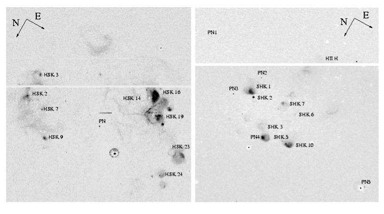
Figure 1: VLT H$\alpha$ - R images of Sextans A (left) and Sextans B (right). The f.o.v. is 2′$\times$2′. The H ii regions and PNe observed spectroscopically are indicated with their identification numbers as in Tab. 1 for H ii regions and as in Magrini et al. (m02 (2002), m03 (2003)) for PNe.

1 Introduction

Sextans A and Sextans B are both dwarf irregular galaxies (Ir V and Ir IV-V morphological types, respectively, cf. van den Bergh bergh (2000), hereafter vdB00) with approximately the same V luminosity and located at a very similar distance (1.3 Mpc, Dolphin et al. dolphin (2003) for Sextans A and vdB00 for Sextans B). Their separation in the sky is also relatively small ($\sim$ 10 degrees), which corresponds to about 280 kpc at the adopted distance. Moreover their velocity difference is only 23 $\pm$6 km s^-1. All these properties suggest a common formation for these two galaxies, probably together with NGC 3109 and the Antlia galaxy, also at a similar distance and location in the sky. Considering the mean distance of the four galaxies from the barycentre of the Local Group (LG), 1.7 Mpc, this sub-group is located beyond the zero velocity surface of the LG (cf. vdB00) and can be considered the nearest external group of galaxies. Then these galaxies are particularly interesting as they represent a group of dwarf galaxies relatively isolated from giant galaxies.

In dIr galaxies, star formation is generally active, as shown by the conspicuous number of H ii regions that they contain. There are several photometric and spectroscopic studies of H ii regions in both galaxies. Photometry of H ii regions in Sextans A was obtained by Hodge (hodge74 (1974)), Aparicio & Rodríguez-Ulloa (aparicio (1992)), and Hodge et al. (hodge94 (1994)), the latter one being the most complete survey with 25 H ii regions detected. Hunter et al. (hunter93 (1993)) studied large ionized gas structures outside normal H ii regions, like shells and filaments generated by the action of massive stars through winds and supernova explosions. Spectra of four H ii regions were obtained by Skillman et al. (skillman89 (1989)), from which an oxygen abundance was derived. The brightest H ii regions of Sextans B were first catalogued by Hodge (hodge74 (1974)). Strobel et al. (strobel (1991)) classified twelve H ii regions, whereas oxygen abundance was derived for four H ii regions by Skillman et al. (skillman89 (1989)). Note, however, that these spectroscopic studies were generally not deep enough (except for one or two objects) to allow direct measurement of the nebular electron temperature via detection of the [O iii] 436.3 nm line, causing an important source of uncertainty in the determination of their chemical abundances.

Planetary nebulae (PNe) are known to be good tracers of intermediate-age stellar populations in galaxies. One PN was discovered in Sextans A by Jacoby & Lesser (jacoby81 (1981)), and then reidentified by Magrini et al. (m03 (2003)). In Sextans B, five PNe are known (Magrini et al. m02 (2002)). To date, no spectroscopic studies were done of these PNe.

As remarked by Mateo (mateo (1998)) “No two LG dwarfs have the same star-formation history”. This is true not only when comparing galaxies of different morphological type, luminosity, or mass, but also when comparing galaxies which are very similar in many aspects, as these two dwarf irregulars. In fact, in spite of a probable common origin, Sextans A and Sextans B show a different star formation history as indicated by the different amounts of stars in the various evolutionary phases, and also reflected in the different number of PNe and H ii regions observed. Sextans A possesses a conspicuous old stellar population (10-14 Gyrs ago) and shows evidence for recent star formation starting about 1-2 Gyrs ago, whereas the amount of star formation at intermediate ages (2-10 Gyrs ago) was modest (see also Dolphin et al. dolphin (2003)). On the other hand, Sextans B exhibits a very strong star formation at recent and intermediate ages (1-4 Gyrs ago), together with a very old population (cf. Mateo mateo (1998)). The different numbers of PNe, 5 in Sextans B vs. 1 in Sextans A, was interpreted by Magrini et al. (m02 (2002)) to be consistent with the different star formation histories of the two galaxies for the age range covered by the PN progenitors, Sextans B showing a stronger star formation rate than Sextans A during the past 2-10 Gyrs. The different star formation history might imply a different chemistry. In this paper, we analyze the chemical content of Sextans A and Sextans B, presenting spectroscopic data of PNe, whose progenitors belong to old and intermediate age populations, and H ii regions, representative of the youngest population.

The paper is organized as follows. Sect.2 describes the observations and the data reduction. Sect.3 presents the chemical abundances obtained for PNe and H ii regions, and discusses the implications on the properties and evolution of the galaxies. In Sect.4 the notable case of the PN in Sextans A is examined. The summary is in Sect.5.

Table 1: The observed H ii regions in Sextans A and Sextans B. The centres of the slits are reported. The adopted names of H ii regions are from Hodge at al. (hodge94 (1994)) for Sextans A and from Strobel et al. (strobel (1991)) for Sextans B. The HII region not identified in previous works is labeled as H ii H.

Name	RA	Dec
	J2000.0
Sextans A
HKS2	10:10:53.6	-4:41:16.9
HKS3	10:10:53.8	-4:41:57.2
HKS7	10:10:55.4	-4:41:11.0
HKS9	10:10:57.0	-4:40:30.6
HKS14	10:11:04.1	-4:42:49.3
HKS16	10:11:05.6	-4:42:31.5
HKS19	10:11:06.9	-4:42:17.8
HKS23	10:11:09.2	-4:40:53.2
HKS24	10:11:09.6	-4:41:36.3
Sextans B
SHK1	9:59:57.7	5:19:36.7
SHK2	9:59:58.3	5:19:46.3
SHK3	9:59:59.9	5:20:17.4
SHK5	10:00:00.4	5:20:25.2
SHK7	10:00:00.8	5:19:38.3
SHK6	10:00:02.2	5:19:44.8
SHK10	10:00:03.1	5:20:31.8
H ii H	10:00:05.3	5:17:58.7

2 Observations and data reduction

All PNe known in these galaxies (1 in Sextans A and 5 in Sextans B) and a sample of H ii regions (9 and 8, respectively) have been observed in December 2003 with the 8.2 m VLT (ESO, Paranal) equipped with the FORS2 spectrograph in multi-object spectroscopy (MOS) observing mode. Pre-imaging, needed to create the MOS masks, was first obtained through an H$\alpha$ filter (central wavelength 656.3 nm, FWHM 6.1 nm) and a R filter (655/165.0 nm). The exposure times for each galaxy were 2$\times$120 s in H$\alpha$ and 2$\times$10 s in R. In the continuum-subtracted H$\alpha$$-$R frames, emission-line objects were identified and their position used to build two MOS masks, one per galaxy.

Spectroscopy was then secured during four consecutive nights (22-25 December). The seeing during the observations was 0^′′.8. The MOS mask used to observe Sextans A contained 32 slits and the one for Sextans B 28 slits. The slits had a width of 0.8″, while their length varied from 3″ to 25″, according to the size of the object to be observed and to the crowding of the area of the galaxy. The slits corresponding to compact objects like PNe were extended enough to include also some adjacent sky spectrum. Several independent slits were used to obtain sky spectra to be subtracted from those of extended H ii regions, which completely fill their slitlets. Spectra were obtained using FORS2 with the 300V and 300I gratings, providing ’blue’ and ’red’ spectra with a total coverage from $\sim$320.0 nm to $\sim$1000.0 nm at a reciprocal dispersion of 0.3 nm pix^-1 and an effective resolution of 0.6 nm. For each galaxy, a total of eight exposures were taken: three with the 300V grating (total exposure time 5400 s), three using the 300I one (3600 s), and also two short exposures for each grating (60 s) to avoid saturation of the most intense emission lines, as H$\alpha$ and [O iii] 500.7 nm. A spectrophotometric standard star, GD 108, was observed once in blue and red during two consecutive nights. The data were reduced using the IRAF LONGSLIT tasks and the MIDAS MOS and LONG packages.

2.1 Images

The H$\alpha$-R FORS2 images of Sextans A and Sextans B are shown in Fig. 1. All PNe in Magrini et al. (m02 (2002), m03 (2003)) were re-identified, together with a number of known HII regions. Compared to previous studies (Hodge et al. hodge94 (1994), Strobel et al. strobel (1991)), several new unresolved H$\alpha$ emission-line objects were found in both galaxies. When comparing their coordinates with the images in Magrini et al. (m02 (2002), m03 (2003)), no associated [O iii] emission was found, and therefore we do not consider them as new candidate PNe. We observed spectroscopically two of them, one in Sextans A and one in Sextans B, confirming that they are stars with a very strong H$\alpha$ line in emission. A detailed analysis of these objects via colour-colour diagrams and spectroscopy will be presented in a forthcoming paper.

In Fig. 1, all PNe and H ii regions observed spectroscopically are marked with their identification numbers as in Tab. 1 for H ii regions and as in Magrini et al. (m02 (2002), m03 (2003)) for PNe.

Figure 2: VLT spectrum of the planetary nebula in Sextans A.

Figure 3: VLT spectra of the five planetary nebulae in Sextans B. Identification numbers come from Magrini et al. (m02 (2002))

Figure 4: VLT spectra of four H ii regions in Sextans A.

Figure 5: VLT spectra of another five H ii regions in Sextans A.

Figure 6: VLT spectra of four H ii regions in Sextans B.

Figure 7: VLT spectra of another four H ii regions in Sextans B.

2.2 Spectra

An important feature of this spectroscopic study is the homogeneous set of observational data and analysis method used to measure chemical abundances for both PNe and H ii regions. Furthermore, the VLT allows us to obtain spectra which are deep enough to measure most basic diagnostic emission lines in spite of the significant distance of the galaxies. The electron temperature diagnostic [O iii] 436.3 was measured in all PNe, and in seven H ii regions out of a sample of 17. In few other H ii regions (four in Sextans A and one in Sextans B), an upper limit to the flux of the [O iii] 436.3 line could be derived. The broad spectral coverage, from 320.0 to 1000.0 nm, allowed us the detection of many recombination (H i, He i, He ii) and forbidden lines of several ions of O ([O i], [O ii], [O iii]), S ([S ii],[S iii]), Ar ([Ar iii], [Ar iv]), Ne ([Ne iii]), and N ([N ii]). Note that the [S iii] lines at 906.9 and 953.2 nm are generally blended with saturated atmospheric absorption features. In this case, the heliocentric velocities of both galaxies, 324 kms for Sextans A and 300  km s^-1 for Sextans B, and the excellent sky transparency at these wavelength in Paranal, allowed us to use safely these lines to determine the S⁺⁺ abundances.

The spectra of the PNe are presented in Figs. 2 and 3, and those of H ii regions in Figs. 4, 5, 6, and 7. Identification of some emission lines is labeled. Note the large number of emission lines detected with a good signal to noise ratio, and the relatively strong blue continuum emission visible in a number of H ii regions, which is likely produced by the exciting stars.

It should be noted that although the observations were carried out at relatively low airmasses, the slits were not aligned exactly to the parallactic angle at the time of the observations: for Sextans A the mean difference between the parallactic angle and the position angle of the slits was 45^∘ and the mean airmass was 1.15, while for Sextans B they were 35^∘ and 1.25, respectively. This implies that, given the relatively narrow slit, some amount of light is lost especially in the blue end of the spectra due to differential atmospheric refraction. In order to estimate these light-losses for point sources like PNe, we have calculated the displacement, as a function of wavelength, of the centroid of an object from the midpoint of the slit along the direction perpendicular to its length, using the figures in Filippenko (filippenko82 (1982)). In doing so, we consider that sources are well centred at H$\alpha$, which is the passband at which acquisition images were taken to centre objects in their slitlets for spectroscopy. We have then calculated the amount of light lost (relative to that at H$\alpha$) because of these displacements from the slit centre, assuming a Gaussian point-spread functions with a FWHM which is the seeing of the observing night, and including seeing worsening toward bluer wavelengths.

As expected, the differential light-losses are negligible in the red side of the spectra, while become as large as 75% for Sextans A, and 90% for Sex B, at the shortest wavelength that we consider, which is that of the [O ii] 372.7 doublet. At H$\gamma$, they become as small as 20% and 25%, respectively. We have applied these correction factors to the fluxes of blue lines, and attached an associated error of one third of the correction factor, which is propagated in all quantities (ionic abundances, ionization correction factor) derived using the blue lines. Note that the correction for the interstellar reddening applied to the spectra would by itself at least partially compensates for the atmospheric refraction, by ‘forcing’ the Balmer lines to have the theoretical unreddened flux ratios (although with an estimated extinction value $c_{\beta}$ larger than the real one). Thus for Sextans A the difference between the observed fluxes and the refraction corrected fluxes, both after the reddening correction, amounts to 50% at the wavelength of the [O ii] 3727 doublet and negligible at H$\gamma$ for Sextans A, and of 60% and 10%, respectively, for Sextans B.

In addition, it is important to note that these quite large corrections at the bluest wavelengths do not affect significantly our chemical analysis. In fact, the oxygen total and ionic abundances of the PNe where the [O ii] 372.7 lines were measured change only by a factor much smaller than 0.1 dex, with respect to the values calculated using the observed fluxes. Moreover, once the fluxes were corrected for the effect of the atmospheric refraction, we analyzed the differences of O⁺/O derived from either the [O ii] 372.7 or 733.0 lines, in those PNe which have both doublets measured. The differences resulted to be less than 15%, which implies in the worst case, i.e. in the PN of Sextans A, a difference in the total oxygen abundance of only 0.05 dex.

For extended objects like H ii regions, the effect of atmospheric dispersion is in principle more complex, because light is lost from one side of the slit but is “gained” from the other side. However, the extension of the spectra along the slit length does not show significant changes in surface brightness and excitation on scales of $\sim$1.5 arcsec (after seeing convolution), which is the size of the displacement due to the atmospheric dispersion. Assuming that the HII regions are also similarly homogeneous in the direction perpendicular to the slit at these scales, then the effect of the atmospheric dispersion is negligible at all wavelengths, and therefore no corrections have been applied to the observed nebular spectra.

Line fluxes and their errors are listed in Tables 2 and 3. Errors include the contributions of background noise, sky subtraction, and flux calibration uncertainties. In the case of PNe, errors include the correction for the atmospheric dispersion were applied; they range from 40$\%$ at 370 nm to less than 1$\%$ at 500 nm.

Finally, the observed line fluxes were corrected for the effect of interstellar extinction, adopting Mathis (mathis (1990)) law with $R_{V}$=3.1. $c_{\beta}$, which is the logarithmic difference between the observed and de-reddened H$\beta$ fluxes, was determined comparing the observed Balmer I(H$\alpha$)/I(H$\beta$) ratio with its theoretical value. For the spectra with the higher signal to noise ratio, we considered also the comparison between the observed and theoretical Balmer I(H$\beta$)/I(H$\gamma$) and I(H$\gamma$)/I(H$\delta$) ratios. In these cases $c_{\beta}$ is the weighted average of the three determinations.

2.3 Radial velocities

High-resolution spectroscopic data of three PNe of Sextans B were taken on April, 2002, with AF2/WYFFOS, a multi-object, wide field, fibre spectrograph working at the prime focus of the 4.2 m WHT (La Palma). We used the Echelle grating with a central wavelength of 493.0 nm and a reciprocal dispersion of 0.028 nm/pixel. The total exposure time was 5400 s. The reduction was done with the IRAF DOFIBER package.

The high resolution WHT spectra allowed us to measure the Doppler shift of the [O iii] doublet lines, and in one case also of H$\beta$, in three PNe of Sextans B, namely PN 1, PN 4 and PN 5. The heliocentric radial velocities are listed in Tab.2. They are consistent, within the errors, with the heliocentric radial velocity of Sextans B (300 km/s from NED) and with the H i observations by Huchtmeier et al. (hucht (2003)), confirming that the PNe belong indeed to the galaxy.

Table 2: Observed line fluxes $F_{\lambda}$ of PNe in Sextans A and Sextans B, on a scale where F(H$\beta$)=100.0, and after correcting for atmospheric dispersion effects. ‘:’ indicates uncertain values, and ‘$<$’ upper limits. Associated errors are described in the text. Some nebular quantities are also reported: $c_{\beta}$, the electron density and temperatures T_e([O iii]) and T_e([N ii]), and the heliocentric radial velocity of three PNe where it was measured.

Ion	SexA-PN	SexB-PN1	SexB-PN2	SexB-PN3	SexB-PN4	SexB-PN5
$c_{\beta}$	0.10$\pm$0.01	0.10$\pm$0.02	0.02$\pm$0.02	0.13$\pm$0.01	0.17$\pm$0.03	0.22$\pm$0.01
Ne(cm-3)	2700$\pm$100	-	-	-	-	-
Te([O iii]) (K)	22300$\pm$1000	12800$\pm$2000	16000$\pm$3000	20000$\pm$2000	11300$\pm$3000	12800$\pm$1000
Te([N ii]) (K)	13400$\pm$500	-	-	-	-	-
V (km/s)	-	310$\pm$15	-	-	310$\pm$15	310$\pm$15
372.7 [O ii]	176.$\pm$70	18:	-	-	-	21.$\pm$10
383.5 H9	8.$\pm$4	-	8.$\pm$6	11.$\pm$6	-	-
386.8 [Ne iii]	19.$\pm$6	38.$\pm$10	28.$\pm$7	55.$\pm$5	43.$\pm$7	93.$\pm$5
388.9 He i, H8	28.$\pm$5	16.$\pm$8	21.$\pm$6	32.$\pm$5	24.$\pm$5	16.$\pm$4
396.7 [Ne iii], H7	27.$\pm$3	29.$\pm$7	22.$\pm$7	29.$\pm$4	37.$\pm$5	46.$\pm$3
410.1 H$\delta$	31.$\pm$2	25.$\pm$7	19.$\pm$6	26.$\pm$4	26.$\pm$7	23.$\pm$3
434.0 H$\gamma$	48.$\pm$2	48.$\pm$4	45.$\pm$4	51.$\pm$3	51.$\pm$	45.$\pm$1.6
436.3 [O iii]	23.$\pm$2	8.$\pm$4	13.$\pm$4	16.$\pm$4	7.$\pm$5	11.$\pm$1.9
447.1 He i	1.3$\pm$1	5.$\pm$4	9.$\pm$3	4.$\pm$2	-	5.$\pm$2
468.6 He ii	51.$\pm$2	$<$1	$<$3	$<$2	$<$1	6.$\pm$2
471.2 He i,[Ar iv]	-	-	-	2.$\pm$1	-	-
474.0 [Ar iv]	-	-	-	3.$\pm$2	-	-
486.1 H$\beta$	100.$\pm$1	100.$\pm$4	100.$\pm$4	100.$\pm$1.5	100.$\pm$5	100.$\pm$2
495.9 [O iii]	206.$\pm$1	202.$\pm$3	190.$\pm$4	182.$\pm$1.6	256.$\pm$3	316.$\pm$1.8
500.7 [O iii]	611.$\pm$1	590.$\pm$2	570.$\pm$3	474.$\pm$1	798.$\pm$3	940.$\pm$1.5
520.0 [N i]	38.$\pm$1	-	-	-	-	-
541.1 He ii	4.2$\pm$1	-	-	-	-	-
575.5 [N ii]	24.$\pm$1	-	-	-	-
587.6 He i	8.$\pm$1	16.$\pm$2	17.$\pm$5	15.$\pm$1	15.$\pm$3	22.$\pm$2
630.0 [O i]	71.$\pm$1	3.$\pm$2	3.$\pm$1	-	-	-
636.3 [O i]	24.$\pm$1	-	-	-	-	-
654.8 [N ii]	291.$\pm$1.	-	-	-	-	-
656.3 H$\alpha$	306.$\pm$1.5	302.$\pm$2	290.$\pm$3	312.$\pm$1.3	321.$\pm$3	332.$\pm$1.3
658.4 [N ii]	835.$\pm$1.8	2:	7:	6.$\pm$1.8	4.$\pm$3	12.$\pm$1.2
667.8 He i	3.$\pm$1.6	3.$\pm$2	3.$\pm$1.5	4.$\pm$1	-	3.$\pm$1.5
671.7 [S ii]	5.$\pm$1.6	-	-	-	-	-
673.1 [S ii]	8.$\pm$1.5	-	-	-	-	-
706.5 He i	4.$\pm$1.6	6.$\pm$3	-	10.$\pm$4	4.$\pm$2	3.$\pm$1.5
713.5 [Ar iii]	3.$\pm$3	-	-	3.$\pm$2	-	-
728.1 He i	2.$\pm$2	-	-	-	-	-
732.5 [O ii]	28.$\pm$2	5.$\pm$3	7.$\pm$3	-	11.$\pm$2	-
906.9 [S iii]	7.$\pm$3	-	-	-	2.$\pm$2	-
953.2 [S iii]	19.$\pm$2	-	-	5:	5:	17:

Table 3: Observed line fluxes $F_{\lambda}$, on a scale where F(H$\beta$)=100.0, and nebular parameters of the H ii regions in Sextans A and Sextans B. Symbols are as in Tab. 1.

SexA	HSK2	HSK3	HSK7	HSK9	HSK14	HSK16	HSK19	HSK23	HSK24
$c_{\beta}$	0.0$\pm$0.01	0.23$\pm$0.01	0.13$\pm$0.01	0.0$\pm$0.01	0.05$\pm$0.02	0.14$\pm$0.01	0.05$\pm$0.01	0.21$\pm$0.01	0.0$\pm$0.02
Ne(cm-3)	100$\pm$100	200$\pm$100	$<$100	400$\pm$200	$<$100	$<$100	$<$100	$<$100	100$\pm$100
Te([O iii]) (K)	$<$12000	13000$\pm$3000	17000$\pm$4000	14000:	14000$\pm$1000	$<$14000	$<$13000	-	$<$13000
Ion
372.7 [O ii]	240.$\pm$10	126.$\pm$10	205.$\pm$10	145.$\pm$9	145.$\pm$16	213.$\pm$10	179.$\pm$8	194.$\pm$8	160.$\pm$10
386.8 [Ne iii]	11.$\pm$5	15.$\pm$8	8.$\pm$6	10.$\pm$6	28.$\pm$8	8.$\pm$5	15.$\pm$5	5.$\pm$3	22.$\pm$8
388.9 He i, H8	-	-	9.$\pm$5	15.$\pm$5	21.$\pm$7	15.$\pm$5	8.$\pm$4	10.$\pm$3	18.$\pm$7
396.7 [Ne iii], H7	-	-	14.$\pm$3	10:	-	20.$\pm$4	17.$\pm$3	9.$\pm$2	20.$\pm$8
410.1 H$\delta$	24.$\pm$3	20.$\pm$5	25.$\pm$3	22.$\pm$3	26.$\pm$3	21.$\pm$2	25.$\pm$2	25.$\pm$2	28.$\pm$8
434.0 H$\gamma$	42.$\pm$2	35.$\pm$2	46.$\pm$3	41.$\pm$3	47.$\pm$3	46. $\pm$2	42.$\pm$2	43.$\pm$2	47.$\pm$5
436.3 [O iii]	$<$1	2$\pm$2	3$\pm$3	2.$\pm$3	6.$\pm$3	$<$1	$<$1	-	$<$1
468.6 He ii	$<$1	$<$1	$<$1	$<$1	3:	6:	$<$1	$<$1	$<$1
486.1 H$\beta$	100.$\pm$2	100.$\pm$2	100.$\pm$2	100.$\pm$2	100.$\pm$3	100.$\pm$2	100.$\pm$1	100.$\pm$2	100.$\pm$3
495.9 [O iii]	27.$\pm$2	57.$\pm$2	39.$\pm$2	31.$\pm$2	115.$\pm$3	22.$\pm$2	24.$\pm$1	5.$\pm$3	25.$\pm$3
500.7 [O iii]	84.$\pm$2	159.$\pm$2	120.$\pm$2	94.$\pm$2	340.$\pm$3	65.$\pm$2	72.$\pm$1.5	15.$\pm$2	75.$\pm$3
587.6 He i	-	7.$\pm$2	10.$\pm$2	4.$\pm$2	-	-	-	-	-
630.0 [O i]	-	-	-	-	8.$\pm$2	-	-	-	-
656.3 H$\alpha$	281.$\pm$2	335.$\pm$2	312.$\pm$2	281.$\pm$2	295.$\pm$3	314.$\pm$2	295.$\pm$3	329.$\pm$2	281.$\pm$3
658.4 [N ii]	7.$\pm$2	9.$\pm$3	9.$\pm$2	11.$\pm$2	7.$\pm$3	8.$\pm$2	10.$\pm$3	13.$\pm$2	10.$\pm$3
671.7 [S ii]	18.$\pm$2	16.$\pm$3	17.$\pm$2	17.$\pm$2	17.$\pm$3	24.$\pm$2	26.$\pm$2	22.$\pm$2	26.$\pm$3
673.1 [S ii]	14.$\pm$2	13.$\pm$3	11.$\pm$2	15.$\pm$2	11.$\pm$3	16.$\pm$2	16.$\pm$2	14.$\pm$2	20.$\pm$3
713.5 [Ar iii]	4.$\pm$2	5.$\pm$3	5.$\pm$2	3.$\pm$2	3.$\pm$3	6.$\pm$2	2.$\pm$2	2.$\pm$2	1.$\pm$3
732.5 [O ii]	-	13.$\pm$3	8.$\pm$2	-	14.$\pm$3	-	-	8.$\pm$2	-
906.9 [S iii]	5.$\pm$2	18.$\pm$3	16.$\pm$3	7.$\pm$5	8.$\pm$2	20.$\pm$3	-	8.$\pm$2	-
953.2 [S iii]	14.$\pm$2	50.$\pm$3	42.$\pm$5	18.$\pm$5	-	-	-	-	-
SexB	SHK1	SHK2	SHK3	SHK5	SHK6	SHK7	SHK10	H ii H
$c_{\beta}$	0.0$\pm$0.02	0.13$\pm$0.01	0.30$\pm$0.05	0.16$\pm$0.01	0.30$\pm$0.03	0.12$\pm$0.02	0.29$\pm$0.01	0.15$\pm$0.01
Ne(cm-3)	$<$100	200$\pm$100	$<$100	$<$100	$<$100	300$\pm$100	$<$100	$<$100
Te([O iii]) (K)	13000:	15000:	-	12000$\pm$2000	-	-	-	$<$17000
Ion
372.7 [O ii]	181.$\pm$7	350.$\pm$4	390.$\pm$30	182.$\pm$8	210.$\pm$40	324.$\pm$10	413.$\pm$6	292.$\pm$7
386.8 [Ne iii]	9.$\pm$3	29.$\pm$3	-	17.$\pm$4	-	-	7.$\pm$3	9.$\pm$3
388.9 He i, H8	8.$\pm$2	26.$\pm$2	-	14.$\pm$3	-	-	23.$\pm$2	11.$\pm$3
396.7 [Ne iii], H7	10.$\pm$2	27.$\pm$1	-	20.$\pm$2	-	-	20.$\pm$2	12.$\pm$3
410.1 H$\delta$	13.$\pm$2	34.$\pm$1	-	22.$\pm$2	-	-	30.$\pm$2	19.$\pm$2
434.0 H$\gamma$	27.$\pm$2	53.$\pm$1	-	38.$\pm$2	-	-	47.$\pm$2	40.$\pm$2
436.3 [O iii]	2.$\pm$2	3.$\pm$2	-	3.$\pm$2	-	-	-	$<$1
468.6 He ii	$<$1	$<$1	-	$<$1	-	$<$1	$<$1	-
486.1 H$\beta$	100.$\pm$3	100.$\pm$0.5	100.$\pm$9	100.$\pm$2	100.$\pm$5	100.$\pm$4	100.$\pm$1	100.$\pm$1
495.9 [O iii]	50.$\pm$3	55.$\pm$0.5	17.$\pm$7	86.$\pm$2	35.$\pm$5	12.$\pm$4	9.$\pm$1	15.$\pm$1
500.7 [O iii]	147.$\pm$3	148.$\pm$0.5	52.$\pm$7	264.$\pm$2	113.$\pm$5	30.$\pm$4	23.$\pm$1	38. $\pm$1
587.6 He i	-	16.$\pm$0.5	-	5.$\pm$	-	-	-	7.$\pm$1
656.3 H$\alpha$	272.$\pm$	312.$\pm$0.5	351.$\pm$4	319.$\pm$1.5	351.$\pm$8	310.$\pm$2	350.$\pm$0.5	316.$\pm$1
658.4 [N ii]	5.$\pm$2	15.$\pm$0.5	25.$\pm$4	8.$\pm$1	28.$\pm$7	23.$\pm$2	22.$\pm$1	10.$\pm$1
667.8 He i	-	5..$\pm$0.5	-	-	-	-	-	-
671.7 [S ii]	15.$\pm$2	27.$\pm$1	59.$\pm$4	21.$\pm$2	75.$\pm$8	29.$\pm$3	33.$\pm$1	22.$\pm$1
673.1 [S ii]	9.$\pm$2	22.$\pm$1	43.$\pm$4	15.$\pm$2	53.$\pm$8	24.$\pm$3	21.$\pm$1	16.$\pm$1
706.5 He i	-	4.$\pm$1	-	-	-	-	-	-
713.5 [Ar iii]	4.$\pm$2	12.$\pm$1	-	2.$\pm$2	-	6.$\pm$3	5.$\pm$1	2.$\pm$1
732.5 [O ii]	-	13.$\pm$1	-	9.$\pm$2	-	-	12.$\pm$2	9.$\pm$1
906.9 [S iii]	10.$\pm$3	16.$\pm$1	-	18.$\pm$2	-	-	12.$\pm$2	8.$\pm$2
953.2 [S iii]	24.$\pm$3	41.$\pm$1	-	43.$\pm$2	-	-	36.$\pm$2	21.$\pm$2

3 Chemical abundances of planetary nebulae and H ii regions

3.1 ICF method

Chemical abundances were derived from the spectra by means of Ionization Correction Factors (ICF) method, following Kingsburgh & Barlow (kb94 (1994)), with evaluation of the errors as in Corradi et al. (corradi97 (1997)) and Perinotto & Corradi (perinotto98 (1998)). As mentioned above, the [O iii] 436.3 emission line was always measurable in all PNe with a sufficiently high signal to noise ratio, thus their [O iii] electron temperature, T${}_{e{\rm[O\leavevmode\nobreak\ III]}}$, could be determined. These are listed in Tab. 2; their high values are typical of low-metallicity PNe (c.f. Stasinska stasinska02 (2002)). The [O iii] 436.3 line was also measured in four H ii regions of Sextans A and in three H ii regions of Sextans B, while its upper limit was estimated in four H ii regions of Sextans A and one of Sextans B. Another temperature diagnostic line, [N ii] 575.5 nm line, was observed in the PN of Sextans A, and a corresponding electron temperature T${}_{e{\rm[N\leavevmode\nobreak\ II]}}$ was determined. In this object, T${}_{e{\rm[O\leavevmode\nobreak\ III]}}$ was used in computing chemical abundances with the ICF method for ions which are ionized twice or more times, and T${}_{e{\rm[N\leavevmode\nobreak\ II]}}$ for species only ionized once. The large difference between T${}_{e{\rm[O\leavevmode\nobreak\ III]}}$ and T${}_{e{\rm[N\leavevmode\nobreak\ II]}}$ is typical of high excitation PNe and it was also found in several Galactic PNe (i.e. McKenna et al. mckenna (1996)). Kingsburgh & Barlow (kb94 (1994)) examined how the ratio between T${}_{e{\rm[O\leavevmode\nobreak\ III]}}$ and T${}_{e{\rm[N\leavevmode\nobreak\ II]}}$ behaves with nebular excitation, plotting this ratio versus the He ii 4686 flux. They found a linear relation between these two quantities, as expressed in eq. 3 of their paper. The PN of Sextans A, which is a very high excitation object, follows this relationship.

The [S iii] near-infrared emission lines were detected in 4 PNe and 12 H ii regions. These lines allow a better accuracy in the measurement of sulphur abundance, especially at low metallicities where [S ii] lines are extremely faint.

The ICF method was applied to the whole sample of PNe and to H ii regions where T${}_{e{\rm[O\leavevmode\nobreak\ III]}}$ was measured. Formal errors on the ICF abundances were computed taking into account the uncertainties in the observed fluxes and in the electron temperatures. A discussion of the error propagation computed with the ICF method is in Corradi et al. (corradi97 (1997)).

3.2 Modelling with CLOUDY

PNe and H ii regions were also modelled using the photoionization code CLOUDY 94.00 (Ferland et al. ferland (1998)), assuming a blackbody central star with effective temperature derived using the Ambartsumian’s (ambar (1932)) or Gurzadyan’s (gurzadyan (1988)) methods, and a spherical nebula with constant density. Density was derived from the [S ii] 671.7/673.1 flux ratio, which was measured in all H ii regions and in the PN of Sextans A. For PNe in Sextans B, it was assumed equal to 3000 cm^-3, which can be considered a typical value for Galactic PNe (see e.g. Stanghellini & Kaler stanghe89 (1989)). In addition, we made some tests varying the density of $\pm$1000 cm^-3 with both the ICF and CLOUDY methods, obtaining negligible changes in the computed abundances.

In the model, we include dust typical of Galactic PNe and of the Orion nebula, for PNe and H ii regions, respectively. The accuracy of the CLOUDY method was tested in Magrini et al. (M04 (2004)), who applied it to seven bright Galactic PNe using only the emission lines typically present in extragalactic PN spectra, and compared the results with the chemical abundances obtained with the ICF method by KB94. A good agreement was found in the helium and metals abundances. For further details on the modelling procedure see Magrini et al. (M04 (2004)) and Perinotto et al. (2004a ).

3.3 Results

The chemical abundances derived for the current sample with the ICF and CLOUDY methods are in general agreement with each other, showing the following r.m.s. differences in both galaxies: $\pm$0.01 for He/H (linear), $\pm$0.15 dex for N/H, $\pm$0.1 dex for O/H, $\pm$0.1 dex for Ne/H, $\pm$0.1 dex for S/H,$\pm$ 0.1 dex for Ar/H for both PNe and H ii regions.

The total and ionic abundances, and the ICF of PNe and H ii regions are reported in Tab. 4 and 5. The total abundances for the whole sample of objects computed with both methods, and their mean values are shown in Tab. 6 for PNe and in Tab. 8 and 9 for H ii regions. H ii regions where only the CLOUDY method was applied because of the absence of a reliable determination of the electron temperature are marked with a “$*$” in Tab. 8 and 9. For Sextans B PN 3, ICF(N) and ICF(S) were not computed because the [O ii] lines needed to compute them were not detected, and thus for these elements only the results from CLOUDY are quoted.

In the case of H ii regions, the ICF of He does not take into account the neutral helium, which might be a considerable fraction of the total helium abundance. However, for the H ii regions where T${}_{e{\rm[O\leavevmode\nobreak\ III]}}$ was measured, and therefore where the abundances with the ICF method were computed (HKS3, HKS7, HKS9, HKS14 of Sextans A and SHK1, SHK2, SHK5 of Sextans B), the comparison between the results of ICF and CLOUDY methods shows that the mean contribution of neutral helium is smaller than 20%. This relatively small contribution makes unnoticeable the difference between the two results within our present errors.

According to the definition by Kingsburgh & Barlow (kb94 (1994)) for Galactic PNe, the PN in Sextans A would be classified as a type I PNe in the Peimbert scheme ($\log$(N/O)$>$-0.1), while all PNe in Sextans B would be non-Type I. However, it is clear that this distinction is hardly applicable to extragalactic PNe, which span a much larger range of metallicities.

Table 4: Total and ionic chemical abundances, and ionization correction factors of Sextans A and Sextans B PNe, computed with the ICF method.

	SexA-PN	SexB-PN1	SexB-PN2	SexB-PN3	SexB-PN4	SexB-PN5
He+/H+$\times$102	3.6$\pm$1.1	9.8$\pm$1.5	9.3$\pm$1.5	7.4$\pm$1.5	9.4$\pm$1.3	12.8$\pm$2.
He++/H+$\times$102	4.8$\pm$0.5	0.09$\pm$0.05	0.3$\pm$0.1	0.2$\pm$0.1	0.1$\pm$0.1	0.5$\pm$0.1
He/H$\times$102	8.4$\pm$1.6	9.9$\pm$1.5	9.6$\pm$1.6	7.6$\pm$1.6	0.95$\pm$1.4	13.3$\pm$2.1
N0/H+$\times$105	3.9$\pm$ 1.2	-	-	-	-	-
N+/H+$\times$105	7.1$\pm$ 0.9	0.008:	0.003:	0.03$\pm$0.01	0.015$\pm$0.01	0.04$\pm$0.02
ICF(N)	3.0	72.	19.	-	45.	130.
N/H$\times$105	22.$\pm$10.	0.5:	0.5:	$>$0.03	0.7$\pm$0.5	5.$\pm$3.
O0/H+$\times$105	5.2$\pm$1.1	0.06$\pm$0.01	0.07$\pm$0.01	-	-	-
O+/H+$\times$105	4.3$\pm$1.6	0.13$\pm$0.30	0.27$\pm$0.30	-	0.4$\pm$0.9	0.1$\pm$0.2
O++/H+$\times$105	3.2$\pm$0.3	9.4$\pm$3.6	4.8$\pm$3.5	3.4$\pm$1.9	17.3$\pm$4.	15.9$\pm$4.
ICF(O)	1.7	1.0	1.0	1.0	1.0	1.0
O/H$\times$105	13.0$\pm$3.7	9.6$\pm$3.7	5.2$\pm$3.9	3.5$\pm$2.4	17.8$\pm$5.	16.4$\pm$5.
Ne++/H+$\times$106	9.2$\pm$3.1	150.$\pm$80.	55.$\pm$30.	80.$\pm$60.	30.$\pm$10.	45.$\pm$20.
ICF(Ne)	4.1	1.0	1.1	1.0	1.0	1.0
Ne/H$\times$105	0.38$\pm$0.20	1.6$\pm$1.2	0.6$\pm$0.3	0.8$\pm$0.6	3.$\pm$1.	5.$\pm$3.
S+/H+$\times$107	2.3$\pm$0.8	-	-	-	-	-
S++/H+$\times$107	3.9$\pm$0.8	-	-	0.8$\pm$0.8	0.9$\pm$0.8	2.5$\pm$1.
ICF(S)	1.1	-	-	-	2.5	3.5
S/H$\times$107	7.0$\pm$1.9	-	-	$>$0.8	2.$\pm$1.	9.$\pm$3.
Ar++/H+$\times$108	9.1$\pm$8.7	-	-	19.$\pm$10.	-	-
Ar+++/H+$\times$108	-	-	-	16.$\pm$10.	-	-
ICF(Ar)	1.9	-	-	1.3	-	-
Ar/H$\times$107	1.7$\pm$1.7	-	-	5.$\pm$4.	-	-

Table 5: Total and ionic chemical abundances, and ionization correction factors of Sextans A and Sextans B H ii regions, computed with the ICF method.

	HKS3	HKS7	HKS9	HKS14	SHK1	SHK2	SHK5
He+/H+$\times$102	5.0$\pm$1.0	7.8$\pm$1.2	3.0$\pm$0.5	-	-	12.3$\pm$2.	3.5$\pm$1.0
He++/H+$\times$102	0.09$\pm$0.01	0.09$\pm$0.01	0.09$\pm$0.01	0.3$\pm$0.1	0.09$\pm$0.01	0.08$\pm$0.01	0.5$\pm$0.2
He/H$\times$102	5.1$\pm$1.0	7.9$\pm$1.2	3.1$\pm$0.5	-	-	12.4$\pm$2.	4.0$\pm$1.2
N+/H+$\times$107	2.9$\pm$0.4	3.3$\pm$0.5	4.4$\pm$0.7	2.7$\pm$0.4	2.0$\pm$0.3	6.0$\pm$0.1	2.7$\pm$0.4
ICF(N)	5.5	2.4	2.6	7.2	4.7	2.8	8.7
N/H$\times$107	15.7$\pm$3.0	7.9$\pm$2.0	12.0$\pm$4.0	20.$\pm$7.0	9.5$\pm$3.5	17.$\pm$5.	24.$\pm$8.
O0/H+$\times$105	-	-	-	0.2$\pm$0.1	-	-	-
O+/H+$\times$105	0.6$\pm$0.1	0.7$\pm$0.1	0.5$\pm$0.1	0.6$\pm$0.1	0.6$\pm$0.1	1.0$\pm$0.1	0.7$\pm$0.1
O++/H+$\times$105	2.7$\pm$0.9	0.8$\pm$0.3	0.9$\pm$0.3	3.8$\pm$1.3	2.3$\pm$0.8	1.8$\pm$0.6	4.3$\pm$1.5
ICF(O)	1.0	1.0	1.0	1.0	1.0	1.0	1.0
O/H$\times$105	3.3$\pm$1.0	1.5$\pm$0.4	1.4$\pm$0.4	4.5$\pm$1.5	3.0$\pm$0.9	2.8$\pm$0.7	5.0$\pm$1.6
Ne++/H+$\times$106	7.0$\pm$2.0	1.4$\pm$0.5	2.1$\pm$0.8	7.7$\pm$2.7	3.5$\pm$1.3	7.5$\pm$2.7	8.1$\pm$2.9
ICF(Ne)	1.2	1.7	1.7	1.2	1.3	1.6	1.2
Ne/H$\times$105	9.0$\pm$5.0	2.4$\pm$1.3	3.5$\pm$1.9	8.9$\pm$5.0	4.4$\pm$2.6	1.8$\pm$0.6	9.5$\pm$5.0
S+/H+$\times$107	1.4$\pm$0.2	1.5$\pm$0.2	2.0$\pm$0.3	1.6$\pm$0.2	1.3$\pm$ 0.1	3.0$\pm$0.5	1.80$\pm$0.2
S++/H+$\times$107	6.0$\pm$1.0	6.0$\pm$1.7	3.2$\pm$0.9	3.5$\pm$0.9	4.9$\pm$ 1.2	7.5$\pm$2.	6.50$\pm$1.6
ICF(S)	1.3	1.1	1.1	1.4	1.25	1.1	1.5
S/H$\times$107	9.2$\pm$2.0	8.0$\pm$2.0	5.7$\pm$1.3	7.2$\pm$1.6	7.8$\pm$ 1.9	11.6$\pm$3.	12.2$\pm$3.
Ar++/H+$\times$107	1.0$\pm$0.3	0.7$\pm$0.2	0.8$\pm$0.2	0.8$\pm$0.2	1.1$\pm$ 0.3	3.2$\pm$ 0.4	0.5$\pm$0.1
ICF(Ar)	1.9	1.9	1.9	1.9	1.9	1.9	1.9
Ar/H$\times$107	1.9$\pm$0.7	1.2$\pm$0.5	1.5$\pm$0.5	1.5$\pm$0.5	2.1$\pm$0.7	5.9$\pm$ 2.	0.9$\pm$0.3

Table 6: Total chemical abundances of Sextans A and Sextans B PNe computed with both ICF and CLOUDY methods. We also report the unweigthed average of the two results. Metal abundances are expressed in 12+$\log$(X/H).

Name	He/H	N/H	O/H	Ne/H	S/H	Ar/H
SexA-PN
ICF	0.084$\pm$0.016	8.35$\pm$0.2	8.1$\pm$0.1	6.6$\pm$0.2	5.8$\pm$0.1	5.2$\pm$0.4
CLOUDY	0.095$\pm$0.02	8.4$\pm$0.2	8.0$\pm$0.1	6.7$\pm$0.2	5.9$\pm$0.2	5.2$\pm$0.2
Average	0.09$\pm$0.02	8.4$\pm$0.2	8.0$\pm$0.1	6.7$\pm$0.2	5.9$\pm$0.2	5.2$\pm$0.3
SexB-PN1
ICF	0.099$\pm$0.015	6.7:	8.0$\pm$0.15	7.2$\pm$0.3	-	-
CLOUDY	0.10$\pm$0.02	6.6:	8.1$\pm$0.3	7.3$\pm$0.3	-	-
Average	0.10$\pm$0.02	6.6:	8.1$\pm$0.2	7.3$\pm$0.3	-	-
SexB-PN2
ICF	0.096$\pm$0.016	6.7:	7.7$\pm$0.3	6.8$\pm$0.2	-	-
CLOUDY	0.11$\pm$0.02	6.6:	8.0$\pm$0.2	7.0$\pm$0.3	-	-
Average	0.10$\pm$0.02	6.6:	7.8$\pm$0.2	6.9$\pm$0.3	-	-
SexB-PN3
ICF	0.076$\pm$0.016	$>$5.5${\dagger}$	7.5$\pm$0.3	6.9$\pm$0.3	$>$4.9${\dagger}$	5.7$\pm$0.2
CLOUDY	0.09$\pm$0.02	6.5$\pm$0.3	7.6$\pm$0.2	7.1$\pm$0.2	5.2:	5.5$\pm$0.2
Average	0.08$\pm$0.02	6.5$\pm$0.3	7.5$\pm$0.2	7.0$\pm$0.2	5.2:	5.6$\pm$0.2
SexB-PN4
ICF	0.095$\pm$0.014	6.8$\pm$0.3	8.3$\pm$0.1	7.4$\pm$0.1	5.3$\pm$0.2	-
CLOUDY	0.09$\pm$0.02	6.3$\pm$0.3	8.2$\pm$0.2	7.4$\pm$0.2	5.2$\pm$0.2	5.1:
Average	0.09$\pm$0.02	6.5$\pm$0.3	8.2$\pm$0.2	7.4$\pm$0.2	5.2$\pm$0.2	5.1:
SexB-PN5
ICF	0.13$\pm$0.02	7.5$\pm$0.3	8.2$\pm$0.1	7.6$\pm$0.2	5.4$\pm$0.2	-
CLOUDY	0.13$\pm$0.02	7.0$\pm$0.3	8.2$\pm$0.2	7.6$\pm$0.2	5.7$\pm$0.2	-
Average	0.13$\pm$0.02	7.3$\pm$0.3	8.2$\pm$0.1	7.6$\pm$0.2	5.5$\pm$0.2	-
Average Sextans B	0.10$\pm$0.02	6.8$\pm$0.6	8.0$\pm$0.3	7.3$\pm$0.3	5.3$\pm$0.4	-

The modelling with CLOUDY also allowed us to estimate some stellar parameters as the luminosity and temperature of the exciting stars, as described by Magrini et al. M04 (2004) . We remind briefly how T_⋆ and L_⋆ were computed in the modelling with CLOUDY. The luminosity of the central star was set to reproduce the observed absolute flux of the [O iii] $\lambda$5007 nebular line, measured by Magrini et al. (m02 (2002), m03 (2003)) via aperture photometry, and reddening-corrected, while the BB T_⋆ was set to match the He i/He ii line ratio.

Using these parameters, the PNe were located in the $\log$T_⋆-$\log$L_⋆ diagram and compared with the available H-burning and He-burning evolutionary tracks for Z=$0.004$ from Vassiliadis & Wood (vass (1994)), as shown in Fig. 8. The obtained T_⋆ and $\log$(L_⋆/L_⊙) are reported in Table 7. Typical errors obtained with the CLOUDY modelling are of the order of 0.15 for $\log$T_⋆ and of 0.25 for $\log$L_⋆.

Table 7: T_⋆ and L_⋆ of the PNe in Sextans A and Sextans B as derived with the modelling with CLOUDY.

Galaxy	Name	T⋆ (K)	$\log$(L⋆/L⊙)
Sextans A	PN	194000	3.9
Sextans B	PN1	61000	3.5
	PN2	78000	3.3
	PN3	72000	3.5
	PN4	65000	3.2
	PN5	90000	3.6

The mass of the core of the PN in Sextans A is distinctively larger than for the PNe in Sextans B, and would imply a progenitor initial mass of $\sim$2-3.5M_⊙, using the initial-to-final mass relation adopted by Vassiliadis & Wood (vass (1994)). The relatively large mass of the progenitor is also typical of type I Galactic PNe (Corradi & Schwarz corradi95 (1995)).

The PNe of Sextans B can be instead associated with less massive cores. Among them, PN 5 seems to have the most massive one. Note, however, that the metallicity of Sextans A and Sextans B, 0.001 and 0.002, respectively, is significantly lower than for the models of Vassiliadis & Wood (vass (1994)), and therefore evolutionary tracks for such low metallicities would be needed for a deeper analysis. ¿From Fig. 8 and the initial to final mass relationship used by Vassiliadis & Wood (vass (1994)), we find that the central stars of Sex B PNe had initial masses between 0.9 and 1.5M_⊙. Stars with these masses and with an initial metallicity Z=0.001 were born between about 10 and 2 Gyr ago (cf. Charbonnel et al. charbo (1999); charbo96 (1996)). As the mean oxygen abundance of PNe in Sextans B is equal, within the errors, to that of H ii regions, this would mean that no noticeable chemical enrichment has occurred in the galaxy since long time ago.

3.4 Comparison with previous determinations of chemical abundances

In Sextans A, Skillman et al. (skillman89 (1989)) observed spectroscopically four H ii regions, deriving 12 + $\log$O/H=7.49. The same spectroscopic data were used by Richer & McCall (richer95 (1995)) to recalculate 12 + $\log$O/H=7.55$\pm$0.11 and by Pilyugin (pil01 (2001)) who obtained through the P-method (Pilyugin pilyugin00 (2000)) 12 + $\log$O/H=7.7. An analysis of supergiant stars by Kaufer et al. (kaufer (2004)) derived a total metallicity which is 1.09 dex lower than solar. A red giants metallicity [Fe/H]=-1.9$\pm$0.4 was derived by Grebel (grebel00 (2000)). Dolphin et al. (dolphin (2003)) found through modeling of the color-magnitude diagram a mean metallicity of [M/H]$\sim$-1.4. These values are in good agreement with 12 + $\log$O/H=7.6$\pm$0.2, the average oxygen abundance derived from our observations of nine H ii regions, corresponding approximately to [Fe/H]=-1.6. The transformation from [O/H] to [Fe/H] needed to compare our nebular oxygen abundances with the stellar abundances was computed according to the empirical transformation by Mateo (mateo (1998)). We used the solar abundances from Grevesse & Sauval (grevesse (1998)) to derive [O/H] from the measured 12 + $\log$O/H. The oxygen abundance of the PN in Sextans A is significantly higher (12 + $\log$O/H=8.0$\pm$0.1), and will be discussed in Sect.4.

In Sextans B, the observations by Skillman et al. (skillman89 (1989)) of four H ii regions gave 12 + $\log$O/H=7.56, while Moles et al. (moles90 (1990)) measured 12 + $\log$O/H=8.1 in a single H ii region. Pilyugin (pil01 (2001)) recalculated both abundances obtaining 12 + $\log$O/H=7.85 and 7.87, respectively. The average oxygen abundance derived in this paper with eight H ii regions is 7.8$\pm$0.2 and from five PNe is 8.0$\pm$0.3, thus in agreement with Moles et al. (moles90 (1990)) and Pilyugin (pil01 (2001)).

A recent very work about spectroscopy of H ii regions and PNe of Sextans A and Sextans B is by Kniazev et al. (kniazev05 (2005) The authors derived chemical abundances of the PN and of three H ii regions in Sextans A, and of one PN (PN3) and three H ii regions in Sextans B with the ICF method. In Sextans A, they found an oxygen abundance of 8.02$\pm$0.05 in the PN and 7.54$\pm$0.06 in three H ii regions, that, we did not observe. These H ii regions belong to the same complex of HSK14, HSK16, and HSK19, for which we derived a mean 12 + $\log$O/H=7.65$\pm$0.1. In PN3 of Sextans B they derived 12 + $\log$O/H=7.47$\pm$0.16, in agreement with our value 7.5$\pm$0.2. They also observed the same H ii regions for which we derived chemical abundances with the ICF method, SHK1, SHK2, SHK5, finding 12 + $\log$O/H 7.50$\pm$0.08, 7.55$\pm$0.06, 7.84$\pm$0.05, respectively. These values are similar to our ICF determinations: 7.5$\pm$0.1, 7.5$\pm$0.1, 7.7$\pm$0.1.

Figure 8: H-burning (dashed lines) and He-burning (continuous line) evolutionary tracks for metallicity Z=0.004 from Vassiliadis & Wood (vass (1994)). Final mass of the central star are quoted close to the corresponding track. Large symbols (circles) correspond to Sextans B PNe and the small one (square) indicates the Sextans A PN.

3.5 Relationships between chemical abundances

The relation between He/H and N/O is shown in Fig. 9, where the observed chemical abundances of PNe are compared with new models by Marigo (2004, private communication) built for initial metallicities Z=0.001 and Z=0.004. Both models predict, for a progenitor mass below 3M_⊙, an enhancement of O/H compared to N/H, producing a N/O abundance ratio decreasing with He/H. At even higher mass progenitors, N/O increases quickly and significantly as the result of hot-bottom burning. The abundance of the PN of Sextans A is in good agreement with the model Z=0.001 and an initial mass around 4M_⊙. Four of Sextans B PNe match within 1-1.5$\sigma$ with the same model, Z=0.001, and masses between 0.55 and 3 M_⊙; one of them, PN 5, is in better agreement with the model with Z=0.004 and a progenitor with initial mass of about 1.5M_⊙, in agreement with the result obtained with the evolutionary tracks (Fig. 8). Note however that the mean metallicity of Sextans B is Z=0.002.

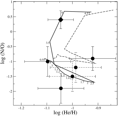
Figure 9: Relationship between He/H and N/O. The solid line is the stellar model for the progenitor by Marigo (2004) for Z=0.001 and the dashed line for Z=0.004. Values of the initial masses are indicated. Full circles correspond to Sextans B PNe and the diamond is the Sextans A PN. PNe with uncertain N/H determination are marked with dot-dashed error bars.

Fig.10 shows the relationship between N/O and N/H for PNe in several nearby galaxies. This relation is well defined for PNe with a slope near to unity, suggesting that the increase of N/O with N/H is due to the increase of N, without modifying the oxygen abundance through the ON cycle. Theoretical predictions of N/O vs N/H for different masses of the progenitor stars and metallicity (Groenewegen & de Jong groene (1994) for the LMC metallicity, and Marigo marigo01 (2001) for Z=0.004) are also shown. The theoretical predictions of Groenewegen & de Jong (groene (1994)), shown by the solid line in Fig.10, and of Marigo (marigo01 (2001)), the dashed line, do not extend to the low metallicities of Sextans A and Sextans B. Because of it, we can only say that models, in particular those of Marigo, (marigo01 (2001)) predict the deviation from the linear relationship of Henry (henry89 (1989)) that the observations of PNe in Sextans B and in the Magellanic Clouds suggest at the lowest metallicities. From the figure there is no indication of oxygen enrichment for PNe with low metallicity and very low mass progenitors (M$<$1.3 M_⊙), as also predicted by theoretical models of Marigo (marigo01 (2001)). The location n the diagram of the Sextans A PN is a clear indication of a large nitrogen production, as expected from its higher mass progenitor, while oxygen production is not evident from this diagram.

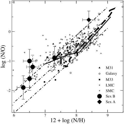
Figure 10: Relationship between N/O and N/H for PNe. The central dot-dashed line is the fit from Henry (henry90 (1990)) using a sample of PNe of the Galaxy, LMC, SMC and M31. The external dot-dashed lines are placed at a distance of $\pm$3$\sigma$ from the fit, where $\sigma$=0.1 dex. The solid line is the model for LMC by Groenewegen & de Jong (groene (1994)) built for the LMC metallicity and several initial masses. The top-right point of the curve corresponds to a model with an initial mass of 8.5 M_⊙, the first change of slope with 2 M_⊙, and the last point (bottom-left) is for 0.93 M_⊙. The dashed line is the model for Z=0.004 and initial masses from 0.8 (left) to 5 (right) M_⊙ by Marigo (marigo01 (2001)). Observed abundances are from: Galaxy (Perinotto et al. 2004a ); LMC and SMC (Leisy et al., in prep.); M31 (Jacoby & Ciardullo jc99 (1999)); M 33 (Magrini et al. M04 (2004)); Sextans A and Sextans B (this work). PNe of Sextans B with uncertain N/H determination are marked with dot-dashed error bars.

Fig. 11 presents the relation between O/H and Ne/H. It is usually believed that the progenitors of PNe do not produce significant amount of oxygen and neon during their lifetime. In fact, the abundances of these two elements seem to vary in lockstep, where the slope of the $\log$-$\log$ relation is very close to unity (cf. Henry henry89 (1989)). This behaviour is essentially the same for H ii regions and it seems independent of the host galaxy. In Fig. 11 the solid line is the fit built with a sample of 157 PNe in the Galaxy, LMC, SMC and M 31 taken from Henry (henry89 (1989)). The dotted lines are placed at a distance of $\pm$1$\sigma$ from the fit, and the dashed lines at $\pm$3$\sigma$, where $\sigma$=0.1 dex. The PNe and the H ii regions of Sextans A and Sextans B appear to follow the “universal” relation.

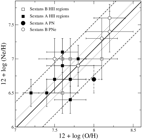
Figure 11: Relationship between Ne/H and O/H. The solid line is the fit built by Henry (henry89 (1989)). The dotted lines are placed at a distance of $\pm$1$\sigma$ from the fit, and the dashed lines at $\pm$3$\sigma$, where $\sigma$=0.1 dex as indicated by Henry henry89 (1989). Only H ii regions with T_e measured are reported.

Table 8: The chemical abundances of H ii regions in Sextans A. Where the electron temperature is measured, values derived with both the CLOUDY and the ICF methods are indicated. In the remaining cases, marked with a “$*$”, only the determinations done with CLOUDY are listed. In computing the average abundances, upper limits of individual determinations are not considered.

Name	He/H	N/H	O/H	Ne/H	S/H	Ar/H
HKS2*
CLOUDY	$<$0.05	6.1$\pm$0.3	7.7$\pm$0.2	6.7$\pm$0.2	6.1$\pm$0.2	5.3$\pm$0.3
HKS3
ICF	0.05$\pm$0.01	6.2$\pm$0.1	7.5$\pm$0.1	6.9$\pm$0.2	6.0$\pm$0.1	5.3$\pm$0.1
CLOUDY	0.05$\pm$0.02	6.3$\pm$0.3	7.6$\pm$0.2	6.6$\pm$0.3	6.1$\pm$0.2	5.3$\pm$0.3
Average	0.05$\pm$0.02	6.2$\pm$0.2	7.5$\pm$0.1	6.7$\pm$0.2	6.0$\pm$0.2	5.3$\pm$0.2
HKS7
ICF	0.08$\pm$0.01	5.9$\pm$0.2	7.2$\pm$0.2	6.4$\pm$0.2	5.9$\pm$0.1	5.1$\pm$0.3
CLOUDY	0.07$\pm$0.02	6.2$\pm$0.3	7.6$\pm$0.2	6.6$\pm$0.3	6.0$\pm$0.2	5.4$\pm$0.3
Average	0.07$\pm$0.02	6.1$\pm$0.3	7.4$\pm$0.2	6.5$\pm$0.2	6.0$\pm$0.2	5.3$\pm$0.3
HKS9
ICF	0.03$\pm$0.01	6.1$\pm$0.2	7.2$\pm$0.2	6.5$\pm$0.2	5.8$\pm$0.1	5.2$\pm$0.3
CLOUDY	0.03$\pm$0.02	6.5$\pm$0.3	7.3$\pm$0.2	6.5$\pm$0.3	5.8$\pm$0.2	5.1$\pm$0.3
Average	0.03$\pm$0.02	6.3$\pm$0.2	7.2$\pm$0.1	6.5$\pm$0.2	5.8$\pm$0.2	5.1$\pm$0.3
HKS14
ICF		6.3$\pm$0.2	7.7$\pm$0.1	7.0$\pm$0.2	5.9$\pm$0.2	5.2$\pm$0.3
CLOUDY	$<$0.05	6.3$\pm$0.3	7.9$\pm$0.2	7.0$\pm$0.3	6.1$\pm$0.2	5.2$\pm$0.3
Average	$<$0.05	6.3$\pm$0.3	7.8$\pm$0.1	7.0$\pm$0.2	6.0$\pm$0.2	5.2$\pm$0.3
HKS16*
CLOUDY	$<$0.05	6.0$\pm$0.3	7.7$\pm$0.2	6.4$\pm$0.2	6.0$\pm$0.2	5.5$\pm$0.3
HKS19*
CLOUDY	$<$0.05	6.2$\pm$0.3	7.6$\pm$0.2	6.9$\pm$0.2	6.2$\pm$0.2	5.0$\pm$0.3
HKS23*
CLOUDY	$<$0.05	6.2$\pm$0.3	7.7$\pm$0.2	6.7$\pm$0.2	5.8$\pm$0.2	5.0$\pm$0.3
HKS24*
CLOUDY	$<$0.05	6.3$\pm$0.3	7.6$\pm$0.2	7.1$\pm$0.2	6.3$\pm$0.2	4.7$\pm$0.3
Average values	0.05$\pm$0.02	6.2$\pm$0.1	7.6$\pm$0.2	6.8$\pm$0.3	6.0$\pm$0.2	5.2$\pm$0.2

Table 9: The same as in Table 8, but for Sextans B.

Name	He/H	N/H	O/H	Ne/H	S/H	Ar/H
SHK1
ICF	-	6.0$\pm$0.2	7.5$\pm$0.1	6.6$\pm$0.2	5.9$\pm$0.2	5.3$\pm$0.2
CLOUDY	$<$0.05	6.1$\pm$0.3	7.6$\pm$0.1	6.5$\pm$0.3	6.0$\pm$0.2	5.3$\pm$0.3
Average	$<$0.05	6.0$\pm$0.2	7.6$\pm$0.1	6.5$\pm$0.2	5.9$\pm$0.4	5.3$\pm$0.3
SHK2
ICF	0.12$\pm$0.02	6.2$\pm$0.2	7.5$\pm$0.1	7.0$\pm$0.2	6.2$\pm$0.2	5.8$\pm$0.2
CLOUDY	0.11$\pm$0.02	6.4$\pm$0.3	7.7$\pm$0.1	7.0$\pm$0.3	6.2$\pm$0.2	5.8$\pm$0.3
Average	0.11$\pm$0.02	6.3$\pm$0.2	7.6$\pm$0.1	7.0$\pm$0.2	6.2$\pm$0.2	5.8$\pm$0.3
SHK3*
CLOUDY	$<$0.05	6.7$\pm$0.3	8.0$\pm$0.2	-	6.7$\pm$0.2	-
SHK5
ICF	0.04$\pm$0.01	6.4$\pm$0.2	7.7$\pm$0.1	7.0$\pm$0.2	6.0$\pm$0.2	4.9$\pm$0.2
CLOUDY	0.04$\pm$0.02	6.3$\pm$0.3	7.7$\pm$0.1	7.0$\pm$0.3	6.1$\pm$0.2	5.0$\pm$0.3
Average	0.04$\pm$0.02	6.3$\pm$0.2	7.7$\pm$0.1	7.0$\pm$0.2	6.0$\pm$0.2	5.0$\pm$0.3
SHK7*
CLOUDY	$<$0.05	6.4$\pm$0.3	7.7$\pm$0.2	-	6.1$\pm$0.2	5.5$\pm$0.3
SHK6*
CLOUDY	$<$0.05	6.6$\pm$0.3	7.8$\pm$0.2	-	6.6$\pm$0.2	-
SHK10*
CLOUDY	$<$0.05	6.4$\pm$0.3	8.1$\pm$0.2	7.0$\pm$0.2	6.0$\pm$0.2	5.5$\pm$0.3
H iiH*
CLOUDY	0.05$\pm$0.02	6.1$\pm$0.3	7.8$\pm$0.2	6.9$\pm$0.3	6.0$\pm$0.2	5.0$\pm$0.3
Average values	0.07$\pm$0.04	6.4$\pm$0.2	7.8$\pm$0.2	7.0$\pm$0.2	6.1$\pm$0.5	5.5$\pm$0.4

3.6 The distribution of chemical abundances within the galaxy

As star formation in dwarf irregular galaxies is thought to be episodic, and the solid-body nature of the rotation inhibits efficient mixing, it is plausible that there are large abundance variations in different regions of a galaxy (Skillman et al. skillman89 (1989)). However, in several dwarf and low-mass galaxies it has been found that the O/H abundance appears surprisingly homogeneous. There are several explanations which can be considered, as described, for example, by Kobulnicky (kobul (1998)). This is true also in the case of Sextans A and Sextans B. The abundance of their best measured element, oxygen, has a low scatter in H ii regions: the average value is 7.6$\pm$0.2 for Sextans A and 7.8$\pm$0.2 for Sextans B, being, therefore, consistent within errors with an uniform distribution.

Another aspect to be considered is the so called ”abundance gap”, which is the difference between the abundances of H ii regions and PNe (cf. Richer et al. richer97 (1997)). Generally H ii regions have larger O/H than PNe, because they belong to a younger population than the PN progenitors, which are not considered to produce large amount of oxygen, unless under “special” circumstances (see Sect. 4). From the models of Richer et al. (richer97 (1997)), this gap is expected to be as large as 0.2 or 0.3 dex, but it is a function of the metallicity and of the chemical history of the galaxy. Both in Sextans A and Sextans B this gap does not seem to be present (for Sextans A, we considered Ne/H instead of the oxygen abundance, which might be enhanced during the evolution of the progenitor of the PN, see discussion in Sect. 4). For Sextans A, its PN has a young, relatively massive progenitor and thus it is not surprising that it has abundances similar to those of H ii regions.

For Sextans B, the old ages of the PNe progenitors estimated in sect. 3.3, together with their homogeneous abundances, would indicate a very low chemical enrichment of the galaxy during a long period of time till the present. Determining with more accuracy the length of this period of low chemical enrichment (5-10 Gyrs?) is prevented by the significant uncertainties and approximations done in deriving the ages of the PN progenitors.

The average O/H abundances of HII regions in Sextans A and Sextans B are slightly different (7.6$\pm$0.2 vs. and 7.8$\pm$0.2, respectively), but they are within the errors and computed dispersion, and therefore no clear indication of a different chemical history can be drawn. In fact, as Sextans A and Sextans B have approximately the same V-luminosity and the same morphological type, considering the well known linear relationship between the metallicity and the luminosity of galaxies (see Pilyugin pil01 (2001)), they are expected to have the same O/H, within the dispersion of the empirical relationship. So the similar O/H abundances, in spite of quite different SFHs, seem to confirm that galaxies with a similar luminosity have similar metallicity and that the luminosity-metallicity relationship represents the ability of a given galaxy to keep the products of its own evolution rather than its ability to produce metals (Larson larson74 (1974)).

4 The peculiar PN of Sextans A

The PN of Sextans A shows significant N/H and O/H overabundances with respect to the H ii regions. N/H is generally enhanced in PNe by nucleosynthesis processes in the progenitor star. The large amount of N/H in this PN can be explained, as for Type I PN in the Galaxy (Corradi & Schwarz corradi95 (1995)), by a relatively high mass progenitor which produces and dredges-up nitrogen. On the other hand, the abundances of neon, sulphur, and argon, which are not expected to be varied by nucleosynthesis, are similar, within errors, to the average values of H ii regions (or slightly lower, consistently with the fact the PN belongs to a slightly older stellar population).

The overabundance of oxygen is more difficult to understand. As noted in Sect. 3.6, the O/H abundance of the H ii regions studied in Sextans A has a low dispersion, indicating that there is today an homogeneous distribution of elements in the galaxy. These data, however, do not allow us to exclude the existence of a metallicity gradient through Sextans A, because the H ii regions are located roughly in a ring, and there are no data for the central region where the PN is located (it should also be remembered that the PN progenitor may have been migrated from its original place of birth). Existing information from the literature appears contradictory, as while the three A-type supergiant stars located over a length of 0.8 kpc studied by Kaufer et al. (kaufer (2004)) have uniform Fe/H abundances, other stars show a larger r.m.s scatter in metallicity at all ages (up to 0.4 dex for intermediate mass stars, Dolphin et al. dolphin (2003), or for red giant branch stars, Grebel et al. grebel (2003)). However, the hypothesis that the progenitor of the PN has formed in a region of Sextans A with locally enhanced metallicity seems to be ruled out (or at least weakened) by the fact that only O/H is significantly higher than in HII regions, while the abundance of other elements which do not vary during stellar evolution of the PN progenitor, like sulphur, argon, and neon, are all very similar to those of the H ii regions.

An alternative, interesting explanation is that O/H surface enrichment occurred during the evolution of the PN progenitor. This was first suggested by Leisy et al. (leisy02 (2002)) for several PNe in the Magellanic Clouds and interpreted as a consequence of a dredge-up that depends on the metallicity of the PN progenitor and enriches of oxygen its surface. Indeed, contrary to “classical” stellar evolution theories, recent semi-analytical models do predict O enrichment by core processed material brought to the surface by the third dredge-up (cf. Marigo marigo01 (2001), Herwig herwig04 (2004)). In the model of Marigo (marigo01 (2001)), the O production depends on several parameters: the metallicity (increasing at low metallicities), the mixing length, and the number of dredge-up episodes (which also increases at low metallicities because of the larger duration of the AGB phase). At a given progenitor mass of 2M_⊙, Marigo (marigo01 (2001)) found an increase of the total oxygen stellar yield of a factor 10, when lowering the initial metallicity from solar to Z=0.004. The oxygen enrichment becomes important only for progenitors with M$>$1.3M_⊙. In a recent paper, Herwig (herwig04 (2004)) computed intermediate mass (from 2 to 6 M_⊙) stellar evolution tracks from the main sequence to the tip of the AGB for starts with extremely low metallicities, namely Z=0.0001. These models predict that oxygen is enhanced in the envelopes of low metallicity AGB stars by the third dredge-up. The new model of Marigo (2004, private communication), built for an initial metallicity Z=0.001 (that of Sextans A), also predicts that the third dredge-up produces some oxygen enrichment, as seen by the slight decreasing trend of N/O with increasing He/H in Fig.9. In particular, for a PN with a progenitor of about 3.5 M_⊙ and an initial metallicity of Z=0.001, Marigo (2004) found that hot bottom burning and third dredge-up are present. The production of oxygen is essentially due to the third dredge-up and it amounts to about 0.4 dex, in (surprisingly good) agreement with the difference found between the PN and the H ii regions of Sextans A. Concluding, our observations of the PN in Sextans A support the possibility that a significant oxygen surface enrichment can occur during the evolution of highest mass PN progenitors born in low metallicity environments. This potentially important result is nevertheless based on the only known example of a PN with a high mass progenitor belonging to such a low metallicity galaxy as Sextans A. Confirming this results is an important objective of future observational research in the field.

5 Summary

In this paper we presented an homogeneous spectroscopic study of ionized nebulae (H ii regions and PNe) representative of populations of different ages, in the two low-metallicity, dwarf irregular galaxies Sextans A and Sextans B. Our main results are:

• i) we have computed, via ICF and CLOUDY modeling, helium, nitrogen, oxygen, neon, argon, and sulphur abundances both in H ii regions and PNe. In particularly, the element with the most accurate determination, oxygen, has the same average value, within the errors, in the PNe and H ii regions of Sextans B: 12 + $\log$(O/H)=8.0$\pm$0.3 and 7.8$\pm$0.2, respectively, indicating a very low metal enrichment during a significant fraction of the galaxy lifetime. For the H ii regions of Sextans A we obtained 12 + $\log$(O/H)=7.6$\pm$0.2, whereas it is 0.4 dex larger for the only PN known there;

• ii) the dispersion of O/H in Sextans A and Sextans B H ii regions has a r.m.s. scatter of 0.2 dex, which is consistent, within the errors, with an uniform distribution;

• iii) the oxygen overabundance of the PN in Sextans A with respect to HII regions might indicate an efficient third dredge-up for massive, low-metallicity PN progenitors as predicted by models of Marigo (marigo01 (2001), 2004).

- (1) Ambartsumian, V. A., 1932, Poulkovo Obs. Circ 4, 8
- (2) Aparicio, A. & Rodríguez-Ulloa, J. A., 1992, A&A, 260, 77
- (3) Charbonnel, C., Meynet, G., Maeder, A. &, Schaerer, D., 1996, A&AS, 115, 339
- (4) Charbonnel, C., Meynet, G., Maeder, A., Schaller, G., & Schaerer, D., 1993, A&AS, 101, 415
- (5) Charbonnel, C., Dåppen, W., Schaerer, D., Bernasconi, P. A., Maeder, A., Meynet, G., Mowlavi, N., 1999, A&AS, 135, 405
- (6) Corradi R. L. M. & Magrini L., 2004, to appear in the proceedings of the ESO-workshop on “Planetary Nebulae beyond the Milky Way”
- (7) Corradi, R. L. M. & Schwarz, H., 1995, A&A, 293, 871
- (8) Corradi, R. L. M., Perinotto, M., Schwarz, H. E., Claeskens, J.-F, 1997, A&A, 322, 975
- (9) Dolphin, A. E., Saha, A.. Skillman, E. D., Dohm-Palmer, R. C., Tolstoy, E., Cole, A. A., Gallagher, J. S., Hoessel, J. G., Mateo, Mario, 2003, AJ, 126, 187
- (10) Dopita, M. A., 1996, Proceedings of the Second Recontres du Vietnam, Editions Frontieres, edited by J. Tran Thanh Van, L. M. Celnikier, Hua Chon Trung, S. Vauclair, p. 295.
- (11) Exter, K. M., Barlow, M. J., & Walton, N. A., 2004, MNRAS, 349, 1291
- (12) Ferland, G. J., Korista, K. T., Verner, D. A., Ferguson, J. W., Kingdon, J. B., Verner, E. M., 1998, PASP, 110, 761
- (13) Filippenko, A. V., 1982, PASP, 94, 715
- (14) Grebel, E. K., 2000, in Star Formation from the Small to the Large Scale, ed. F. Favata, A. A. Kaas, & A. Wilson (SP-445) (Noordwijk: ESA), 87
- (15) Grebel, E. K., Gallagher, J. S. III, & Harbeck, D., 2003, AJ, 125, 1926
- (16) Grevesse, N. & Sauval, A. J., 1998, SSRv, 85, 161
- (17) Groenewegen. M. A. T. & de Jong, T., 1994, A&A, 282, 127
- (18) Gurzadyan, G. A., 1988, ApSS, 149, 343
- (19) Henry, R. B. C., 1989, MNRAS, 241, 453
- (20) Henry, R. B. C., 1990, ApJ, 356, 229
- (21) Herwig, F., 2000, ApJ, 605, 425
- (22) Herwig, F., 2004, ApJS, 155, 651
- (23) Hodge, P. W., 1974, ApJS, 27, 113
- (24) Hodge, P., Kennicutt, R. C., & Strobel N., 1994, PASP, 106, 765
- (25) Huchtmeier, W. K., Karachentsev, I. D., Karachentseva, V. E., 2003, A&A, 401, 483
- (26) Hunter, D. A., Hawley, W. N., & Gallagher, J. S., 1993, AJ, 106, 1797
- (27) Kaufer, A., Venn, K. A., Tolstoy, E. Pinte, C., Kudritzki, R.-P., 2004, AJ, 127, 2723
- (28) Kingsburgh, R. L. & Barlow, M. J., 1994, MNRAS, 271, 257
- (29) Kniazev, A. Y., Grebel, E. K., Pustilnik, S. A., Pramskij, A. G., Zucker, D. B., 2005, astro-ph/0502562
- (30) Kobulnicky, H. A., 1998, ASPC, 147, 108
- (31) Jacoby, G. H. & Lesser, M. P., 1981, AJ, 86, 185
- (32) Jacoby, G. H., Ciardullo, R,, 1999, ApJ, 515, 169
- (33) Larson, R. B., 1974, MNRAS, 169, 229
- (34) Leisy, P., Francois, P., & Dennefeld, M., 2002, RMAA, 12, 140
- (35) Magrini, L., Corradi, R. L. M., Walton, N. A., et al., 2002, A&A, 386, 869
- (36) Magrini, L., Corradi, R. L. M., Greimel, R., et al., 2003, A&A, 407, 51
- (37) Magrini, L., Perinotto, M., Mampaso, A., Corradi, R. L. M., 2004, A&A, 426, 779
- (38) Marigo, P., 2001, A&A, 370, 194
- (39) Marigo, P., Bressan, A., & Chiosi, C., 1996, A&A, 313, 545
- (40) Mateo, M. L., 1998, ARA&A, 36, 435
- (41) Mathis J.S. 1990, ARA&A 28, 37
- (42) McKenna, F. C., Keenan, F. P., Kaler, J. B., Wickstead, A. W., Bell, K. L., & Aggarwal, K. M., 1996, PASP, 108, 610
- (43) Moles, M., Aparicio, A., & Masegosa, J., 1990, A&A, 228, 310
- (44) Pagel, B. E. J., 1998, in “Nucleosynthesis and chemical evolution of galaxies”, Cambridge Univ. Press, 1998, pag.289
- (45) Perinotto, M., Corradi, R. L. M., 1998, A&A, 332, 721
- (46) Perinotto, M., Morbidelli, L., Scatarzi, A., 2004A, MNRAS, 349, 793
- (47) Perinotto, M., Magrini, L., Mampaso, A., Corradi, R. L. M., 2004B, to appear in the Proceedings of the ESO-workshop “Planetary Nebulae beyond the Milky Way”
- (48) Pilyugin, L. S., 2000, A&A, 362, 325
- (49) Pilyugin, L. S. 2000, A&A, 362, 325
- (50) Pilyugin, L. S., 2001, A&A, 374, 412
- (51) Richer, M. P. & McCall, M. L., 1995, ApJ, 445, 642
- (52) Richer, M. P. & McCall, M. L., 2004, to appear in the Proceedings of the ESO-workshop “Planetary Nebulae beyond the Milky Way”
- (53) Richer, M. G., McCall, M. L., Arimoto, N., 1997, A&AS, 122, 215
- (54) Skillman, E. D., Kennicutt, R. C., & Hodge, P. W., 1989, ApJ, 347, 875
- (55) Stanghellini, L. & Kaler, J. B., 1989, ApJ, 343, 811
- (56) Stasinska, G., 2002, in the Proceedings of “Ionized Gaseous Nebulae”, Eds. W. J. Henney, J. Franco, M. Martos, & M. Peña, RMAA 12, 62
- (57) Strobel, N. V., Hodge, P., & Kennicutt R. C. Jr., 1991, ApJ, 383, 148
- (58) Tosi, M., Greggio, L., Marconi, G., & Forcardi, P., 1991, AJ, 102, 951
- (59) van den Bergh, S., 2000 in The Galaxies of the Local Group, Cambridge University Press, vdB00
- (60) Vassiliadis, E. & Wood, P. R., 1994, ApJS, 92, 125