How Far Away are Gravitational Lens Caustics? Wrong Question

Abstract

It has been a persistent question at least for a decade where the gravitational lens caustics are in the radial direction: whether in front of the lensing mass, behind the lensing mass, or on the plane normal to the line of sight that passes through the lensing mass, the radiation source, or the observer. It is a wrong question. And, the truth angers certain referees who somehow possess the ability to write lengthy rubbish referee reports and delay certain papers indefinitely.

General relativity is a metric theory, particularly of Riemannian geometry, which is characterized by the existence of an inner product – or, the invariance of the proper time. According to Einstein field equations, a compact mass defines a spherical geometry around it and focuses photons from a distant source to an observer with the source and observer as the two focal points. When the mass is spherically symmetric, the two dimensional lens equation that relates the angular positions of a source and its images defines a point caustic at the angular position of the lensing mass. The third (radial) position of the point caustic is not defined. For an arbitrary mass, the caustic extends into a web of piecewise smooth curves punctuated by cusps and again its notion exists only within the context of the lens equation. We point out a few errors in a couple of papers, published in the Astrophysical Journal, which may be influential.

Subject headings: gravitational lensing

1 Spherical Geometry and Focal Points

If we consider a 2-sphere, the geodesics (“straight lines”) are the great circles and any two great circles intersect in two places that are known as antipodal points in geography. There are no parallel geodesics on the sphere, and that is the well-known break-down of the fifth axiom (or postulate; see section 1.1) of plane geometry (or Euclidean geometry). Given a pair of antipodal points such as north pole and south pole, there are infinitely many geodesics that diverge from one antipodal point and converge to the other. The antipodal points are the foci of the geodesics.

The 2-sphere ($S^{2}$) is characterized by a constant Gaussian curvature, and Gaussian curvature is nothing but the Riemann curvature scalar where the non-unity constant between them is just a matter of historical conventions. In two dimensions, Riemann curvature tensor has only one independent component, and the Einstein tensor is given in terms of the Riemann curvature scalar and “trivial tensor structure” built from metric components. For the homogeneous space $S^{2}$, the scalar curvature is constant – Gauss curvature. (Weinberg, p.144; Weinberg hereafter)

Just for a moment, let’s stipulate for the purpose of illustration that the longitudes on $S^{2}$ are photon paths between a radiation source at the north pole and an observer at the south pole. A image of an object an observer sees in its detector (say an array of light receptors including counters with $100\%$ efficiency, perfect homogeneity, and infinite resolution) is a distribution of photons on the detector that last-scattered the object (the last-scattering surface either of a radiation emission source that generates the photons, or of a reflecting object such as a planet, etc) whose image the observer seeks. Thus, if we assume that the radiation emission source at the north pole emits photons isotropically, the image of the radiation emission source (of the radius of a “point”) that the observer at the south pole sees in its detector will be a circle (unless the detector is set exactly at the focal point and is burned; if the emission is directional such as in lasing, the image will not be a circle because most of the geodesics that connect the source and observer will not be followed by the photons from the “point” source.)

When the observer visits the north pole, the observer will find through meticulous measurements around the north pole that the radiation source has the size of a “point” and the shape of the radiating surface is not a circle. If we allow the observer and source for the third dimension around the north pole for the sake of imagination, the observer will be able to take a mugshot of the radiation surface which will show up as a “point” in its detector. In fact, the observer will most likely bring a lab-prepared isotropically emitting “point” light source to set up at the north pole and confirm that the “point source” indeed produces a circular image when measured at the south pole.

This dimensional change from a zero-dimensional point source to a one-dimensional circular image results in the point caustic of a spherically symmetric lensing mass in the context of the lens equation as we shall review in the following section.

It should be useful to note that focal points are also referred to as conjugate points. For example, two antipodal points are a pair of conjugate points; Or, the south pole is the conjugate point of the north pole.

1.1 Axioms of Euclid Geometry

We list the five axioms of Euclid which can be found in Euclid’s textbook Elements written around 300 BC and had been used well into the 20th century.

1. A straight line can be drawn from any point to any point.

2. In a straight line, a finite straight line can be produced continuously.

3. A circle with any center and radius can be described by introducing a straight line segment as the radius and one of its end points as the center.

4. All right angles equal one another.

5. If a straight line falling on two straight lines makes the interior angles on the same side less than two right angles, the two straight lines, if produced indefinitely, meet on that side on which are the angles less than the two right angles.

In order to avoid causing unnecessarily rigid authoritative impression of the five postulates (or axioms) of Euclid, we remark that the axioms of plane geometry have evolved. For example, seek the axioms by George Birkhoff who is perhaps better known for Birkhoff theorem (that the metric of a spherically symmetric mass is static and given by Schwarzschild metric). We should further note that Euclid was reluctant to use the fifth axiom and his postulates are sometimes known as 4+1 postulates. Considering the length of the fifth axiom, it is tempting to jump to a “fuzzy axiom” that simplicity is the beauty of truth.

2 The Lens Equation of a Spherically Symmetric Mass

2.1 Newtonian Deflection Angle

In 1911, following up on his 1907 article on the gravitational influence on the propagation of light, Einstein published a calculation of the gravitational deflection angle by the Sun in an article titled “Über den Einfluss der Schwerkraft auf die Ausbreitung des Lichtes,” Annalen der Physik, 35. Einstein got the deflection angle too small by factor 2 by considering the gravitational effect on the clock correctly but omitting the effect on the measuring rod. In other words, he got Newtonian deflection angle. It was before the systematic exposition of the general relativity culminating in what are now referred to as Einstein field equations (1916). We take it as a historical lesson that we resort to the Einstein field equations whenever in doubt.

The masslessness of the light particles or $U(1)$ gauge invariance was not known in the era of Newton, but Newton’s equation of motion of two particles under the mutual gravitation in the center of mass coordinates can be “naturally” extended to describe the motion of a massless photon under the gravitational influence of a mass $M$. If the masses of the two particles are $m_{1}$ and $m_{2}$, and their reduced mass is $m:\ m^{-1}=m_{1}^{-1}+m_{2}^{-1}$, the motion of the reduced mass $m$ (with relative position vector $x=r\hat{r}$) is given by two equations in spherical coordinates where the scattering plane is chosen by $\theta=\pi/2$.

$$m\,E={m\over 2}\dot{r}^{2}+{m\over 2}{J^{2}\over r^{2}}-{m\,GM\over r}\ ;\qquad m\,J=m\,r^{2}\dot{\varphi}\ ,$$ (1)

where $E$ and $J$ are the (conserved) energy and angular momentum per unit reduced mass, and $M$ is the total mass.

For the motion of photons, divide the equations with the reduced mass $m\neq 0$ and consider the resulting equations in the limit of $m\rightarrow 0$. If impact parameter is denoted $b$ (as usual),

$$b\equiv\lim_{t\rightarrow-\infty}r\sin\,(\varphi-\varphi_{-})$$ (2)

where $\varphi_{-}\equiv\varphi(t=-\infty)$. The energy and angular momentum of the photon can be determined from $b$ and eq. (1) with $t=-\infty$.

$$E={1\over 2}\ ;\qquad J=b\ .$$ (3)

The stationary condition $\dot{r}=0$ has one solution because $E>0$, and that is the distance ($r_{0}$) of the closest approach of the photon to the mass $M$.

$$r_{0}=-GM+(G^{2}M^{2}+J^{2})^{1/2}$$ (4)

Since $J>0$, the azimuthal angle increases with time ($\dot{\varphi}>0$).

The equation of the orbit can be found by a simple integration of eq. (1) after eliminating $dt$. For the incoming photon,

$$\int_{\varphi_{-}}^{\varphi}d\varphi=\int_{\infty}^{r}-{dr\over r^{2}}\left(1+{2GM\over r}-{J^{2}\over r^{2}}\right)^{-1/2}\ ,$$ (5)

and the equation of the orbit is given by

$$\varphi-\varphi_{-}=\cos^{-1}\left({-B\over A}\right)-\cos^{-1}\left({r^{-1}-B\over A}\right)\ ,$$ (6)

where $B\equiv GMJ^{-2}$ and $A\equiv(J^{-2}+B^{2})^{1/2}$. If $\varphi_{0}\equiv\varphi(r_{0})$, the photon trajectory is reflection symmetric with respect to the periastron, and its deflection angle is given by

$$\delta\varphi=2(\varphi_{0}-\varphi_{-})-\pi=2\cos^{-1}\left({-B\over A}\right)-\pi\ .$$ (7)

The equation of the orbit can be rewritten in terms of $\varphi_{0}$ and results in the standard equation of a conic.

$${1\over r}={GM\over J^{2}}\left(1+e\cos(\varphi-\varphi_{0})\right)\ ;\qquad e\equiv\left(1+{J^{2}\over G^{2}M^{2}}\right)^{1/2}$$ (8)

where $e$ is the eccentricity of the conic section. $e>1\ (E=1/2>0)$ and the orbit is hyperbolic. In terms of the eccentricity,

$$\delta\varphi=2\cos^{-1}\left(-{1\over e}\right)-\pi\ ,$$ (9)

and for $J<<GM$, in the linear order of $GM/J$,

$$\delta\varphi={2GM\over J}={2GM\over b}={2GM\over r_{0}}\ .$$ (10)

This is the Newtonian deflection angle of the photon trajectory due to mass $M$. It is inversely proportional to the distance of the periastron $r_{0}$ correctly, but the numerical factor is wrong by factor 2. The correct formula is $\delta\varphi=4GM/r_{0}$ and can be obtained from Einstein field equations.

(The scope of the notations $A$ and $B$ used in this subsection solely for the purpose of visual compactness of the expressions is limited to this subsection.)

2.2 Einstein Deflection Angle

The Schwarzschild metric was found in 1916 promptly after the publication of Einstein’s general relativity (Weinberg, Chap. 8), and Birkhoff theorem states that the metric of any spherically symmetric mass is static and given by the Schwarzschild metric (Weinberg, Chap. 11). Thus, we prefer to derive the Einstein deflection angle by a spherically symmetric mass $M$ by using the exact metric solution of a mass $M$ instead of the Einstein’s method of approximation in the 1916 thesis. The standard form of the Schwarzschild metric is given by

$$ds^{2}=-Bdt^{2}+Adr^{2}+r^{2}d\theta^{2}+r^{2}\sin^{2}\theta d\varphi^{2}\ ;\qquad B=A^{-1}=1-{2GM\over r}\ .$$ (11)

A photon trajectory is a null geodesic in the metric, and the equation of motion (geodesic equation) can be obtained by the variational principle from the path integral of the Lagrangian ${\cal L}$.

$$S=\int{\cal L}dp=\int{1\over 2}g_{\mu\nu}\dot{x}^{\mu}\dot{x}^{\nu}dp\ ,$$ (12)

where $g_{\mu\nu}$ is the metric tensor component, $\dot{x}^{\mu}\equiv dx^{\mu}/dp$, and $p$ parameterizes the path $x(p)$. We can define the canonical momenta

$$P_{\mu}\equiv{\partial{\cal L}\over\partial\dot{x}^{\mu}}\ ,$$ (13)

and Nöther’s theorem guarantees that the time component $P_{t}$ and the azimuthal component $P_{\varphi}$ are conserved along the motion since the Lagrangian is independent of $t$ and $\varphi$. We also can define Hamiltonian and it is conserved because the Lagrangian does not depend on the path parameter $p$ explicitly.

$${\cal H}\equiv P_{\mu}\dot{x}^{\mu}-{\cal L}={\cal L}={1\over 2}P_{\mu}P^{\mu}={1\over 2}{ds^{2}\over dp^{2}}\ ,$$ (14)

The last equality shows that the invariance of the Hamiltonian is nothing but the invariance of the proper time $d\tau$. For the massless photons, $0=d\tau^{2}=-ds^{2}$, and $P^{2}=P_{\mu}P^{\mu}=0$.

$$P_{t} = -B\,\dot{t}={\rm constant}\equiv-E$$ (15)

$$P_{\varphi} = r^{2}\sin^{2}\theta\,\dot{\varphi}={\rm constant}\equiv EJ$$ (16)

$$P_{\theta} = r^{2}\dot{\theta}$$ (17)

$$P_{r} = B^{-1}\dot{r}$$ (18)

$$P^{2} = -B\dot{t}^{2}+B^{-1}\dot{r}^{2}+r^{2}\dot{\theta}^{2}+r^{2}\sin^{2}\theta\,\dot{\varphi}^{2}={\rm constant}=0$$ (19)

Since the metric is isotropic, choose an orbital plane by setting $\theta=\pi/2$  ($\dot{\theta}=0$). Eliminate $dt$ and $dp$ from the equations of $P_{t}$, $P_{\varphi}$, and $P^{2}$, and integrate the resulting equation to obtain the equation of the orbit. The procedure is similar to that of the Newtonian scattering in the previous subsection (except that the integral can not be expressed in terms of elementary functions) and can be found in any textbooks on general relativity (e.g., Weinberg, Chap. 8). In the linear regime $r>>GM$, we obtain the Einstein deflection angle

$$\delta\varphi={4GM\over r_{0}}\ ,$$ (20)

where $r_{0}$ is the distance of the periastron of the photon trajectory. It is worth noting that $g_{tt}=-B$ and $g_{rr}=A^{-1}$ equally contribute to the Einstein deflection angle, and the Newtonian deflection angle amounts to the contribution from $g_{tt}$. The factor 2 discrepancy between the Newtonian and Einstein deflection angles are the well-known general relativistic factor 2, which was tested in 1919 during the eclipse notably by Eddington and his crew and numerously since.

It should be useful to note that the variation of the action $S$ in eq. (12) leads to the “standard” geodesic equation,

$$0=\ddot{x}^{\lambda}+\Gamma^{\lambda}_{\mu\nu}\dot{x}^{\mu}\dot{x}^{\nu}\ ,$$ (21)

where $\Gamma^{\lambda}_{\mu\nu}$ is the affine connection. Hence the path parameter $p$ is a so-called affine parameter which is a linear function of the proper time. If we choose an arbitrary parameter, the equation develops extra terms as one can check easily.

2.3 The Lens Equation

The source star and the observer are far away from the lensing mass $M$, and there the metric is effectively flat. The coordinates have been chosen such that $B,\,A\rightarrow 1$ as $r\rightarrow\infty$, hence the observer should feel relaxed to use the familiar flat space coordinate systems to make local measurements or to chart the sky knowing that the coordinate systems are valid all the way from the observer’s neighborhood to the neighborhood of the source star except inside the star. In the asymptotically flat coordinate system, the photon arriving at the observer’s detector after a long flight along a null geodesic would seem to come from a position in the sky that differs from the position of the source star where the latter is determined by hypothetically turning off the gravity by setting the Newton’s constant $G=0$. The relation between a source position and its images in the observer’s sky is the lens equation.

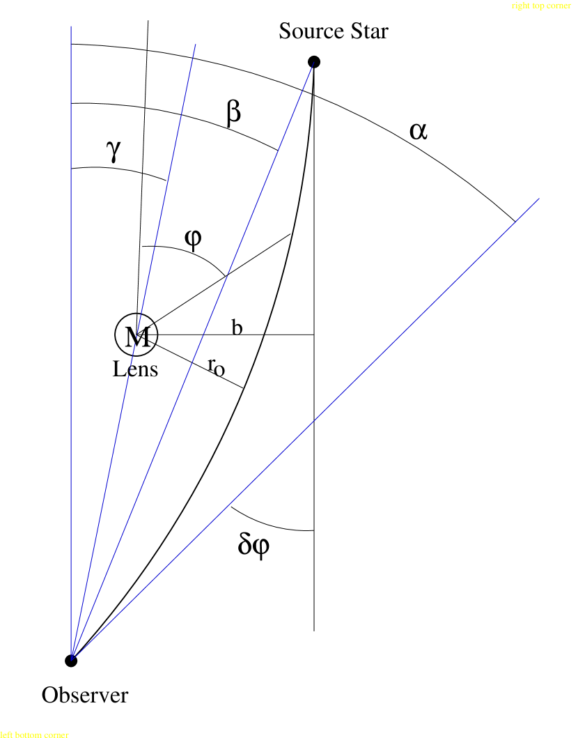
Figure 1: Overlay of an observer’s sky on the orbital plane $\theta=\pi/2$: $b$ is the impact distance, $r_{0}$ is the periastron distance, and $\delta\varphi$ is the deflection angle of the photon trajectory. If the source star is at the angular position $\beta$, the observer sees an image corresponding to the depicted photon trajectory at the angular position $\alpha$. The lens equation shows that there are either two images or two half-circle images, forming a full circle, for a given source position $\beta$. The radius of the circular image is known as Einstein ring radius.

Fig. 1 shows an overlay of the observer’s sky on the orbital plane $\theta=\pi/2$ and a photon trajectory (null geodesic) that connects the source and the observer. The position angles of the lens, source star, and image are depicted as $\gamma$, $\beta$, and $\alpha$, and they are related to $r_{0}$ and $\delta\varphi$ by the followings.

$$b=D_{\ell}\sin(\alpha-\gamma)\ ;$$ (22)

$$D_{s}\sin(\alpha-\beta)=\tan\delta\varphi\left(D_{s}\cos(\alpha-\beta)-D_{\ell}\cos(\alpha-\gamma)-b\tan(\delta\varphi/2)\right)\ ,$$ (23)

where $D_{\ell}$ and $D_{s}$ are the (radial) distances to the lens mass $M$ and the source star from the observer. In the linear order small angle approximation, the equations (22) and (23) become

$$b=D_{\ell}(\alpha-\gamma)\ ;\qquad D_{s}(\alpha-\beta)=\delta\varphi(D_{s}-D_{\ell})\ .$$ (24)

Using the Einstein deflection angle $\delta\varphi=4GM/r_{0}$ and $r_{0}=b-GM\approx b$, the familiar single lens equation is obtained.

$$\alpha-\beta={4GM\over\alpha-\gamma}\left({1\over D_{\ell}}-{1\over D_{s}}\right)\equiv{\alpha_{E}^{2}\over\alpha-\gamma}$$ (25)

Given the angular positions of a source ($\beta$) and a lens ($\gamma$), there are usually two solutions for $\alpha$; the source, lens, and two images are collinear in the sky. If the periastron distance $r_{0}=R_{E}=D_{1}\alpha_{E}$, however, the lens and source are aligned along the line of sight ($\beta=\gamma$), and the image forms on a ring due to the symmetry around the axis connecting the observer and the mass $M$. The angular radius of the ring image is given by $\alpha_{E}$. (There are two solutions $\alpha=\pm\alpha_{E}$ for $\theta=\pi/2$, and the axial symmetry allows two solutions for each value of $\theta=[0,\pi]$ resulting in solutions of two half circles of the same radius $\alpha_{E}$. See section 2.4.1 for a way to understand the transition from two images to two half-circle images.) The circular image is known as Einstein ring, hence the subscript $E$ in $\alpha_{E}$.

The gravity of the mass $M$ makes the geometry of the space around it spherical and focuses photons from the source to the observer; The source and observer are the two focal points of the geodesics that connect them. There are usually two geodesics that connect the source and observer, hence two images of a given source. When the source and lens are aligned (as seen from the observer with $G=0$), infinitely many null geodesics connect the source and the observer, similarly to the longitudes connecting the south and north poles on $S^{2}$ discussed in section 1; The source and observer are the two focal points of the infinitely many photon trajectories, and the observer sees a circular image of the source.

In a following section, we shall see that the Einstein ring is also the critical curve. The caustic is by definition the curve onto which the critical curve is mapped, and the caustic of the single lens is a point caustic since the entire critical curve is mapped to one point under the lens equation. In fact, the point caustic is a degenerate cusp. A cusp is by definition a point onto which a precusp – a critical point where the critical eigenvector is tangent to the critical curve – is mapped.

2.3.1 A Diversion: Einstein Ring or Chwolson Ring?

We find in monograph “Gravitational Lenses”, P. Schneider, J. Ehlers, and E. E. Falco, 1993, p. 4 that Chwolson remarked in “Über eine mögliche Form fiktiver Doppelsterne” of a ring-shaped image of the background star centered on the foreground star. Schneider et al. states that the circular image should be called Chwolson ring instead of Einstein ring.

Chwolson’s main concern in the short article was a spectroscopic double star made of the foreground star and one (faint) image of the background star near the foreground lensing star. We recognize that the title “On a possible form of fictitious double stars” may invoke in the minds of today’s readers of a spectroscopic double star made of the foreground star and the images of the aligned background star instead, which may be more practically referred to as “spectroscopic differentiation of blending”. Chwolson did not consider the lensing effects on the fluxes of the images and also concluded with a sentence “Whether the case of a fictitious double star considered here actually occurs, I can not judge.”

Then, it is very curious what Chwolson might have imagined for the flux of the ring image of which he did not make any statements. If he presumed the same flux as that of the unlensed background star as he did in his article for the (faint) image, what must he have thought of the flux density around the ring? Distribute two background star fluxes around the ring because two images turn into a ring image? Distribute infinitely many point source stars around the ring? Which will result in an infinitely bright point star to an observer with a poor resolution detector such as human eyes? Or, then, distribute finitely many background stars around the ring because the stars have finite sizes? Then, what was the size of the ring? What if the ring size is not an integer multiple of the size of the stars – which in fact will be mostly the case apart from very rare coincidences? We do not have access to Chwolson’s article and can only guess from Schneider et al. that Chwolson must have recognized the axial symmetry but did not have enough details or interest to determine (or conjecture) the radius of the ring image. And, Chwolson was not aware of the lensing effect on the image fluxes. Then, it is possible that Chwolson’s remark on the ring image was mainly to point out the deviated situation from the case of a spectroscopic double star of which the latter was of his interest.

It seems to be quite reasonable to use the term Einstein ring radius since Einstein was the first author to calculate the radius of the circular image. Einstein wrote in 1936 , “An observer will perceive … instead of a point-like star A, a luminous circle of the angular radius $\beta$ around the center of B, where $\beta=\sqrt{\alpha_{0}R_{0}/D}$.” Einstein calculated the ring radius in an approximation where the distance $D$ to the lensing star (e.g., lensing by the Sun) is much smaller than the distance to the source star. ($\alpha_{0}$ is the deflection angle of a photon trajectory grazing the surface of the foreground star and $R_{0}$ is the radius of the foreground star.) Einstein calculated the total magnification of the images (the second equation in the article) and knew that the ring image is luminous. He wrote, “This apparent amplification $q$ … is a most curious effect, not so much for its becoming infinite, … ”, and didn’t seem to have concerned himself with the formal divergence. Physical objects are never a point and physical quantities are never exactly a delta function. In fact, Dirac delta function exists as a distribution which is defined within the context of integration. The third equation in the Science article shows $q=1/x\,(x\rightarrow 0)$ where $x$ is the angular distance between the stars A and B. Integration of the apparent amplification over a small disk ${\cal D}$ centered at $x=0$

$$\int_{\cal D}\Sigma(x_{1},x_{2})\,q\,dx_{1}dx_{2}=\int\Sigma(x_{1},x_{2})\,q\,xdx2\pi$$ (26)

is well-defined and finite as far as the stellar surface flux density $\Sigma(x_{1},x_{2})$ is regular, which indeed is the case.

Then, how do we recognize that Chwolson was aware of and wrote in 1924 that the image would be a ring centered at the foreground star when the foreground and background stars are aligned (always meaning as seen from the observer with $G=0$)? Should we make the recognition by calling the circular image Chwolson ring instead of Einstein ring? We consider a few aspects before casting an intellectually reasonable vote.

• Chwolson ring refers to a circular image. Einstein ring also refers to a circular image. (Precisely speaking, two half-circle images which should be distinguishable by putting trace markers on the background star radiation pattern.) Chwolson mentioned it in 1924, and Einstein calculated it 12 years later in 1936.

• Chwolson ring is an image ring with unspecified radius and unspecified characteristics. Einstein ring is an image ring with a specified radius and flux characteristics determined from the involved physical variables.

• It seems most reasonable to call $\alpha_{E}$ the Einstein ring radius because Einstein is the one who first recognized the importance of the radius and calculated it. Now if we choose to call a ring image a Chwolson ring, the radius of the Chwolson ring may be most naturally called Chwolson ring radius. If Chwolson had studied the characteristics of the image ring (such as the flux) establishing its physical nature and simply left out the radius in his article to be supplemented by, say, Einstein 12 years later, it would be reasonable to call the image ring Chwolson ring and its radius Chwolson-Einstein radius. But Chwolson did not. Considering the historical facts above, then, it may be reasonable to call the image ring Chwolson-Einstein ring and the ring radius Einstein ring radius.

• For general lenses, Einstein ring and Einstein ring radius of a mass do not refer to the shape and radius of an image (or conjoined two images) but refer to an imaginary circle and its radius that function as a scale disk where the functionality derives from the Einstein ring formula Einstein derived for the first time (albeit for a case where the distance to the lensing star is small). Since Chwolson ring is an image ring without physical functionality, it seems too big a leap, for example, to call the Einstein ring of the total mass of a binary lens Chwolson ring.

• Thus, we conclude that it is most reasonable to call Einstein ring and Einstein ring radius Einstein ring and Einstein ring radius in their most general contextual significances as is the current practice. On the other hand, it seems reasonable to call an observational circular image Chwolson-Einstein ring and its ring radius Einstein ring radius. (“Circular images” are being found in cosmological lensings by galaxies – extended mass distributions whose surface densities are not necessarily circularly symmetric, and the “circular images” are not exactly circular even when the emission source is centered at the center of the caustic.)

2.4 The Linear Differential Behavior of the Lens Equation

The lens equation in eq. (25) is written in terms of the variables defined in the orbital plane $\theta=\pi/2$. In order for the lens equation to describe the lensing corresponding to photon trajectories in an arbitrary orbital plane, the lensing variables should be expressed in terms of the two dimensional variables defined in the observer’s sky. If $x$, $s$, and $y$ are the two dimensional angular positions of an image, its source, and the lens, the lens equation is given by

$$x-s=\alpha_{E}^{2}{x-y\over(x-y)^{2}}\ .$$ (27)

In terms of complex coordinates,

$$\omega=z-{\alpha_{E}^{2}\over\bar{z}-\bar{x}_{1}}\ ;\qquad(\alpha_{E}=1)$$ (28)

where $z$, $\omega$, and $x_{1}$ are the complexifications of $x$, $s$, and $y$. It is convenient and customary to normalize the lens equation so that $\alpha_{E}=1$ (as is indicated in the parenthesis).

The lens equation is an explicit function from a two-dimensional image variable to a two-dimensional source variable. In other words, the lens equation is a mapping from a complex plane to itself. The Jacobian matrix of the lens equation describes its linear differential behavior, and when the Jacobian determinant vanishes, the dimension of the vector space of the mapped decreases. In other words, an infinitesimal two-dimensional image is mapped to an infinitesimal source of one-dimension. (The trace of the Jacobian matrix is non-zero, and when one eigenvector vanishes, the other is non-zero – in fact, 2.) The set of points where the Jacobian determinant $J$ vanishes is called the critical curve.

$$J=1-|\kappa|^{2}=1-{1\over|z-x_{1}|^{4}}\ ;\qquad\kappa\equiv{\partial\bar{\omega}\over\partial z}$$ (29)

The critical curve ($J=0$) is a circle of radius 1 ($1=\alpha_{E}$ or $R_{E}$, usually, depending on how to normalize the lens equation) centered at $x_{1}$. In other words, the critical curve coincides with the circular image of the Einstein ring. The critical curve is mapped to $\omega=x_{1}$, hence the lens position is the position of the point caustic. Inversely, a point source at the lens position produces the circular image on the critical curve.

It is useful to define linear Einstein ring with radius $R_{E}\equiv D_{1}\alpha_{E}$ ( mentioned above). The photon trajectories that form the circular image passes through the (linear) Einstein ring at their closest approaches to the mass $M$; in other words, their periastron distances is $r_{0}=R_{E}$.

The Jacobian matrix

$${\cal J}=\pmatrix{1\ \bar{\kappa}\cr\kappa\ 1}$$ (30)

has eigenvalues $\lambda_{\pm}=1\pm|\kappa|$, and the eigenvectors are

$$e_{+}=\pmatrix{E_{+}\cr\bar{E}_{+}}\ ;\quad e_{-}=\pmatrix{E_{-}\cr\bar{E}_{-}}$$ (31)

where

$$\kappa=|\kappa|e^{-i2\theta}\ ;\qquad E_{+}\equiv e^{i\theta}\ ;\qquad E_{-}\equiv iE_{+}\ .$$ (32)

On the critical curve, $|\kappa|=1$ and $\lambda_{-}=0$, and the critical eigenvector $\pm E_{-}$ is tangent to the critical curve at every critical point. (Eigenvectors are not assigned the senses. Thus, $\pm E_{-}$.) In other words, every critical point is a precusp, and the point caustic is a degenerate cusp.

2.4.1 Breaking the Degeneracy with a Small Constant Shear

We break the degeneracy of the point caustic of a point mass by introducing a small constant shear to understand the degeneracy as a limit. Recall how to produce a constant electric field using a dipole where two large opposite charges are separated by a large distance. We can introduce a large mass at a large distance such that $mass/distance^{2}$ is constant, to a similar effect. If the point mass is at $z=x_{1}$ where $x_{1}=0$ is real, and the large mass is on the negative real axis, the lens equation is given by

$$\omega=z+\epsilon\bar{z}-{1\over\bar{z}}\;\qquad\epsilon\geq 0\ .$$ (33)

For our purpose, we need small $\epsilon$. The lens equation (33) known as Chang-Refsdal model  has a bifurcation of the critical curve (hence also caustic curve) at $\epsilon=1$, hence we assume $\epsilon<1$ so as to take a smooth limit of $\epsilon\rightarrow 0$.

$$\kappa=\epsilon+{1\over z^{2}}\equiv|\kappa|\,e^{-2i\theta}$$ (34)

and the critical curve is where $|\kappa|=1$. If $z$ is real, then $\kappa$ is real and positive, hence $\kappa=1$ where the critical curve intersects the real axis (or the “dipole axis”). The critical points on the “dipole axis” are

$$z=\pm(1-\epsilon)^{-1/2}\ ,$$ (35)

and they exist for $\epsilon<1$. The critical eigenvector at the critical points are $\pm E_{-}=\pm ie^{i\theta}=\pm i$ since $\kappa=1\ (\theta=0,\ \pi)$. The tangent to the critical curve at the critical points,

$${dz\over d\theta}=\pm i\,(1-\epsilon)^{-3/2}\ \propto\ \pm E_{-}\ ,$$ (36)

are parallel to the critical eigenvector $\pm E_{-}$, and so the critical points are precusps. The corresponding cusps are at

$$\omega=2\epsilon z=\pm 2\epsilon(1-\epsilon)^{-1/2}\ .$$ (37)

The lens equation has only one singularity (pole) at $z=0$ and its topological charge is 1. There are two limit points where $\kappa=0$, namely, at $z=\pm i\epsilon^{-1/2}$. Thus, the critical curve is made either of one loop enclosing the pole ($\epsilon<1)$ or of two loops each enclosing a limit point ($\epsilon>1)$. One-loop critical curve has topological charge 1 and produces a 4-cusp caustic. Each loop of the two-loop critical curve has topological charge $1/2$ and produces a triangular caustic. The bifurcation from one quadroid to two trioids occurs at $\infty$. Here we are interested in the quadroid because it is the quadroid that contracts to a point in the limit of a point mass lens $\epsilon\rightarrow 0$. The quadroid has two cusps on the real axis given in eq. (37) and it is easy to guess correctly from the symmetry that the other two are on the imaginary axis, reflection symmetric with respect to the “dipole axis”. The quadroid is bisected by the real axis.

Now consider $\omega$ on the real line. There are two real solutions for $z$.

$$0=(1+\epsilon)z^{2}-\omega z-1$$ (38)

For $|\omega|>2\epsilon(1-\epsilon)^{-1/2}$, one solution is negative ($J\leq 0$) and the other is positive ($J\geq 0$). For $|\omega|>2\epsilon(1-\epsilon)^{-1/2}$, both are negative ($J<0$). The lens equation (33) can be embedded into a fourth order polynomial equation for $z$, hence there can be two more solutions. Substitute $z=re^{i\phi}$ and find that the solutions are on a circle centered at the position of the point mass lens element.

$$r^{2}={1\over 1-\epsilon}\ ;\qquad\omega=2\epsilon r\cos\phi$$ (39)

The solutions exist for $|\omega|\leq 2\epsilon(1-\epsilon)^{-1/2}$, which defines the real line segment contained by the two cusps; Inside the quadroid, there are two extra images for each $\omega$ and they are on the circle of radius $(1-\epsilon)^{-1/2}$. They are positive images ($J\geq 0$). The two extra images satisfy the following quadratic equation, which can be found by dividing the fourth order polynomial by the quadratic equation for the real solutions.

$$0=z^{2}-\omega\epsilon^{-1}z+(1-\epsilon)^{-1}$$ (40)

where $\omega$ is real and inside the quadroid caustic.

If we consider $\omega$ moving on the real line in the positive direction and crossing a cusp $\omega=-2\epsilon(1-\epsilon)^{-1/2}$, the positive image on the real line crosses the critical point $z=-(1-\epsilon)^{-1/2}$ into the area enclosed by the critical curve and turns into a negative image. The other image on the real line moves in the positive direction maintaining its (negative) parity until $\omega$ crosses the other cusp $\omega=2\epsilon(1-\epsilon)^{-1/2}$. In the mean time, the two extra images trace the circle: one image, the half-circle in the upper half plane, and the other image, the half-circle in the lower half plane. Figure 2 is a depiction of the Einstein ring as the critical curve of the single point mass lens $M$. Let’s consider the ring, for a moment, as the circle of the two extra images (and imagine the quadroid centered at $M$): the arrow near the point mass lens depicts the motion of the source $\omega$; two arrows on the real line depict the images moving on the real line; two arrows on the ring depict the two extra images that start at one precusp and end at the other precusp.

Now take the limit $\epsilon\rightarrow 0$, and one can visualize two images tracing the Einstein ring instantaneously at the crossing of the point caustic.

We find the above a comfortable (usually involving continuity or traceability) way to think of the transition from two point images to two half-circle images. The criticality of a lens equation in general is related to formation or disappearance of the two extra images (or higher even number of images). In the case of the single point mass lens, the two extra images trace a ring instantaneously forming a ring image due to the degeneracy, and the dimensional change of the linear differential vector spaces of the lens equation is manifested in a global manner.

3 Caustics of Lensing by Slowly Moving Matter

The exquisite symmetry of the Schwarzschild lens (spherically symmetric matter) that led to the caustic of degenerate cusp is readily broken in a more general lens, and the caustic is generally a one-dimensional curve as is the critical curve. The lens equation obtained with the small angle approximation is a mapping of the complex plane (extension of a small neighborhood of the observer’s sky where the small angle approximation is valid) to itself. The criticality condition $J=0$ imposes one constraint reducing the dimension of the variable space by one. Thus, the critical curve is a one dimensional curve which may be a disjoint sum of many loops, and they are usually smooth. Also, the lens equation is usually smooth almost everywhere except at the poles due to the point mass lens elements ($z=x_{1}$ in the case of the single point mass lens discussed above). At the poles, $J=-\infty$, hence it is reasonable to assume that the lens equation is smooth on the critical curve for gravitational lenses in general.

A smooth curve is mapped to a smooth curve by a smooth mapping except at the stationary points of the mapping. Recall that one of the two eigenvectors vanishes on the critical curve. If we consider a small deviation $dz$ from a critical point,

$$dz=dz_{+}E_{+}+dz_{-}E_{-}\qquad\rightarrow\qquad d\omega=d\omega_{+}E_{+}\ ,$$ (41)

hence $\omega$ changes only in the direction of $E_{+}$. Now if $dz_{+}=0$, then $d\omega=0$. So, if we imagine tracing the critical curve (or integrating the tangent to the critical curve) and mapping to draw the caustic curve, the procession of the caustic curve stops momentarily where $dz_{+}=0$ and turns around. In other words, the caustic curve develops a cusp where the tangent to the critical curve is parallel to the critical eigenvector $\pm E_{-}$. The critical point where the tangent has $dz_{+}=0$ is called precusp. Thus, the caustic curve of a lens equation is a piecewise smooth curve punctuated by cusps which may be a disjoint sum of cuspy loops that may intersect themselves.

As the point caustic at the lens position of the single lens is defined within the context of the lens equation, the caustic curve of a general gravitational lens is defined only within the context of the lens equation.

4 Comments on Two Papers

We discuss a couple of papers found in the Astrophysical Journal that may play an unfortunate role of perpetuating misunderstandings.

4.1 “Superluminal Caustics” in 2002

The paper entitled “Superluminal Caustics of Close, Rapidly-Rotating Binary Microlenses”, Zheng Zheng and Andrew Gould, ApJ 541 (2002), 728, considers the caustic curve of the binary lens equation as an object of the size given by the multiplication of its angular size and distance $D_{1}$ and of an (unspecified) inertia whose velocity has to be compared with the speed of light and be concerned of for its tachyonic nature. As we discussed in this article, the caustic is defined only within the context of the lens equation, and especially, it is not an object of an inertia. There is nothing wrong with thinking of the caustic curve as a large linear object by projecting it to the normal plane passing through the source or passing through the lens, or at any distance along the line of sight if that serves to understand or apply the lens equation for some purpose as far as the contextual existence and characteristics of the caustics as defined within the lens equation are valid. Certainly, inertia is not a quality of the caustics defined in the lens equation; There does not exist a tachyonic caustic.

If we stipulate for a moment for the purpose of clearing up another conceptual mistake that the caustics be endowed with inertias, what the caustics can newly acquire is the tachyonic nature but not a superluminal phenomenon known in astrophysics as we discussed in astro-ph/0002414. Zheng and Gould speculate to detect their “superluminal caustics” using very large telescopes such as of 100m aperture. We repeat that tachyonic caustics do not exist; The nomenclature of “superluminal caustic” is a misidentification even within the context of their (mistaken) idea about the motion of the caustics. There does not exist a physically perceivable notion of “superluminal caustic” nor a tachyonic caustic, and it would be an unnecessary waste of resources to consider detecting “superluminal caustics” with say LHT (Larger than Huge Telescope).

Other serious problems of the paper by Zheng and Gould can be found elsewhere.

How is such a paper published in the Astrophysical Journal in 2002? Perhaps, in the same way other worthy papers are smothered in the referee system.

4.2 “Fermat’s Principle” in General Relativity in 1990

The paper entitled “Fermat Principle in Arbitrary Gravitational Fields”, Israel Kovner, ApJ 351 (1990), 114, is cited in the monograph on lensing titled “Gravitational Lenses” by Schneider et al. for Fermat’s principle. Thus, it is likely that the Kovner’s article is influential. Among others, we discuss why “the least proper time principle”, a generic variational principle in general relativity, should not be referred to as Fermat’s principle.

4.2.1 Focal Points of a Gravitational Spherical Geometry are not Caustics

Kovner seems to misidentify the source and observer as the caustics (and “past caustics”) as he states in the second paragraph of section IV, p. 118, “The caustics are mergings of $\geq 2$ extremals of the emission time, … the past-caustics of the past light cone emanating from the observer … .” We discussed above hat the source and observer are the two focal points of a particular set of null geodesics, namely the null geodesics that connect the source and the observer. An observer can see a photon from the source only if the photon arrives at the detector (or the eye) of the observer, and it is imperative that there exist some null geodesics that connect the source and the observer if the observer will be able to image the source photonically. In plane geometry, there is only one (null) geodesic between the two points defined by the source and the observer. In spherical geometry, the geodesics cross, resulting in multiple geodesics connecting two points. There is where the notion of the focal points comes in. They are the focal points of the geodesics of the spherical geometry. Distinct null geodesics produce distinct images, the spherical geometry is responsible for multiple images, and the source and observer are the two foci of the null geodesics corresponding to the multiple images.

The misidentification of the source and observer as caustics may derive from the definition of caustics in electromagnetic lensing. See, for example, “The Classical Theory of Fields”, L. D. Landau and E. M. Lifshitz, 1975, p.133.

4.2.2 Least Action Principle in Non-Relativistic Mechanics

“Fermat’s principle” in general relativity is a four-dimensional version of the least (abbreviated) action principle of the non-relativistic mechanics where the lagrangian has only the kinetic terms.

The principle of least action in non-relativistic mechanics states that the “abbreviated” action

$$S_{0}=\int dt\,P\dot{Q}$$ (42)

of a system for which the Hamiltonian is conserved is the extremum along the equation of the motion. $Q$ is the coordinate variable of the particle and $P$ is its conjugate. Recall that the equations of motion are obtained as the extremum of the action

$$S=\int dt\,L=\int PdQ-Hdt\ .$$ (43)

In a system with conserved Hamiltonian, one can consider only the paths that satisfy the conservation of the Hamiltonian by constraining by the equation of the motion and allowing a variation of the final time $t$ (or final time and initial time: See Goldstein or Landau and Lifshitz), and the (abbreviated) action $S_{0}$ is the action that has an extremum under the variation. If we denote the variation $\Delta$ variation after Goldstein (chap. 7),

$$\Delta S=\left(L-{\partial L\over\partial\dot{Q}}\dot{Q}\right)\Delta t=-H\Delta t\ .$$ (44)

From the second equality of eq. (43) and conservation of $H$,

$$\Delta S=\Delta S_{0}-H\Delta t\ ,$$ (45)

hence $\Delta S_{0}=0$. Now if there is no external force and the kinetic energy is conserved, $S_{0}=2H\int dt$ and the particle follows a path such that the time it takes is the extremum (usually minimum, hence least time principle).

$$0=\Delta S_{0}=2H\Delta t$$ (46)

It recalls Fermat’s principle in geometric optics which is also called the principle of least time.

In order to see the structural parallel (as a functional analysis) with the four-dimensional case of the general relativity, note that Hamiltonian and time variable are a pair of canonical conjugates.

4.2.3 Least Action Principle in General Relativity

The Hamiltonian of the system of a freely falling particle described in eq. (12) is nothing but the (half the) momentum square of the particle and is conserved along the equation of motion. The Hamiltonian ${\cal H}$ and the path parameter $p$ are canonical conjugates. There is no external force for a particle freely falling in a curved space time as defined by the metric, hence this is an exact parallel with the non-relativistic case discussed above where the kinetic energy is conserved. The resulting variational principle is a principle of extremum path parameter $p$, or equivalently a principle of extremum proper time $\tau$. Recall the action in eq. (12) and define $S_{0}$,

$$S=\int{\cal L}dp\ ;\qquad S_{0}=\int P_{\mu}\dot{x}^{\mu}dp\ ,$$ (47)

and the $\Delta$ variation of the action $S$ is given by

$$\Delta S=-{\cal H}\Delta p\ .$$ (48)

Since the Hamiltonian is conserved,

$$\Delta S=\Delta S_{0}-{\cal H}\Delta p\ ,$$ (49)

hence $\Delta S_{0}=0$. From $S_{0}=\int 2{\cal H}dp$,  $0=\Delta S_{0}=2{\cal H}\Delta p$. Expressing in terms of the $\Delta$ variation of the proper time,

$$0=\Delta S_{0}=2{\cal H}\Delta p=-{d\tau^{2}\over dp^{2}}\Delta p=-{d\tau\over dp}\Delta\tau=-(-g_{mu\nu}\dot{x}^{\mu}\dot{x}^{\nu})^{1/2}\Delta\tau\ .$$ (50)

The space-time path taken by the particle is such that the proper time elapsed is in extremum.

$$0=\Delta\int d\tau=\Delta(\tau-\tau_{-})=\Delta\tau$$ (51)

If we consider photons leaving a light source at $\tau=\tau_{-}$, the light paths are determined such that the arrival time $\tau=\tau_{+}$ ( for a given $\tau_{-}$) or the travel time $\delta\tau=\tau_{+}-\tau_{-}$ is an extremum.

One potential pitfall in eq. (51) is the case where $d\tau^{2}=0$ because, then, $0=\Delta S_{0}$ does not necessarily imply $0=\Delta\tau$. We may take the limit $d\tau^{2}\rightarrow 0$ as the case for photons and assume that $0=\Delta\tau$ is valid. Then, we need to confirm that the new action $\int d\tau$ does generate the equations of motion as its extremum.

$$S_{\tau}=\int d\tau=\int{d\tau\over dp}dp=\int(-g_{\mu\nu}\dot{x}^{\mu}\dot{x}^{\nu})^{1/2}dp$$ (52)

Under the variation of the path $x^{\mu}(p)$, the variation of the action is (Weinberg, p.76)

$$\delta S_{\tau}=-\int\left({d^{2}x^{\alpha}\over d\tau^{2}}+\Gamma^{\alpha}_{\mu\nu}{dx^{\mu}\over d\tau}{dx^{\nu}\over d\tau}\right)g_{\alpha\beta}\,\delta x^{\beta}\,d\tau\ .$$ (53)

If a particle follows the equations of free fall, the variation of the action vanishes. In other words, the physical space-time path a particle follows is such that the proper time elapsed is an extremum. Now, there is no ambiguity related to $d\tau^{2}=0$; Photons indeed follow paths for which the travel times (or arrival times for given departure times) are extrema.

1. The last paragraph in p.100 of the monograph “Gravitational Lenses” by Schneider et al. states, “ … does not refer to the ‘time’ a light ray needs to travel from the source to the observer … but a stationary property of the (invariant) time of arrival at the observer … .” Since the arrival time $\tau=\tau_{+}$ and the travel time $\delta\tau=\tau_{+}-\tau_{-}$ are effectively the same variables once given the time of the departure $\tau=\tau_{-}$, it is a self-contradiction. If the arrival time can be defined, so can the travel time. If the arrival time along a geodesic is an extremum, so is the travel time along the same geodesics. Then, why do Schneider, Ehlers, and Falco denounce the notion of travel time while accepting arrival time? It is unclear within the section on “Fermat’s principle” in the book. The source of the error may be $\delta\lambda_{obs}=0$ in the Kovner’s article where Kovner does not elaborate the new action $S_{0}$. ($\lambda$ is the path parameter in Kovner’s.) It is apparent that the error has propagated unchecked.

2. What is conspicuous is that eq. (52) is just another commonly used path integral and variation in general relativity to derive the equations of motion from a variational principle (Weinberg, p.76). The freely falling particle can be massive or massless. For the latter, $d\tau^{2}=0$, and for the former, $d\tau^{2}\neq 0$ which we may normalize such that $d\tau^{2}=1$. Now, should we pluck out, of the continuum (at least classically) of mass spectrum, the massless subset given by $d\tau^{2}=0$ and call it Fermat’s principle? Most certainly not.

3. The evolution of the fundamental physics has been in the direction of unifications. Not only the light but a car is a wave according to quantum mechanics except that the latter has much shorter matter (or de Broglie) wave length. In the limit of zero wavelength, the classical equations are recovered either for massless particles (photons, phonons, etc) or massive particles. Maxwell equations for light lead to the eikonal equation (or geometric optics) in the limit of zero wavelength that is suitable to describe the propagation of the wave front of the light bundle in a medium whose electromagnetic properties vary slowly – usually, wrapped up as a slowly varying refraction index. The eikonal equation can be derived from an action and its variation. It corresponds to a case where the kinetic energy is conserved. Thus, Fermat’s principle, or the principle of least time. (The historical account of Fermat’s principle can be found in a separate article.)

   In general relativity, unlike in Newtonian gravity, the gravitation is not given as an external force but is integrated into the general covariance. It is exactly in the same manner as the electromagnetic forces are integrated into $U(1)$ gauge covariance, for example, in quantum electrodynamics. In this framework of “geometrization”, the forces are integrated into dynamic variables. As a result, the lagrangian ${\cal L}$ in eq. (12) describes a free particle, has only the kinetic terms, which is conserved, and allows simple variations.

4. Geometric optics (or eikonal equation) is exactly valid in the limit of zero wavelengths and can be described by the geodesic equation when under gravity. Huygens principle is about diffraction phenomenon where the wavelengths of the light with respect to the aperture matter: “Huygens wavelets” propagate out as small spherical waves from every point of the aperture (with a subtle understanding of the nature of the approximation that the point is sufficiently smaller than the aperture and is sufficiently larger than the wavelength). It is unclear how the “Huygens wavelets” are related to light cones and “Fermat’s principle” as Kovner states in p.116, “Another way to regard the Fermat principle for light is provided by the Huygens principle as illustrated in Figure 2.” Does Kovner imply that diffractions are also described by geometric optics?

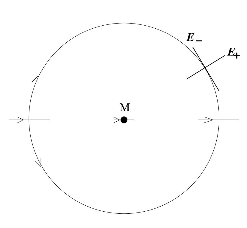
Figure 2: Einstein ring as the location of the ring image and critical curve. $\pm E_{+}$ is the positive eigenvector (for $\lambda_{+}$) and radial, and $\pm E_{-}$ is the negative eigenvector (for $\lambda_{-}$) and tangential. As the source crosses the point caustic along the real line, two images on the real line reach two critical points, then two images instantaneously trace the Einstein ring at the crossing as the two arrows on the ring indicate, and two images move on along the real line. The last: one toward the lens position and the other toward $\infty$.