Turbulence and Magnetic Fields in Astrophysical Plasmas

1 Introduction

Magnetic fields permeate the Universe. They are found in planets, stars, accretion discs, galaxies, clusters of galaxies, and the intergalactic medium. While there is often a component of the field that is spatially coherent at the scale of the astrophysical object, the field lines are tangled chaotically and there are magnetic fluctuations at scales that range over orders of magnitude. The cause of this disorder is the turbulent state of the plasma in these systems. This plasma is, as a rule, highly conducting, so the magnetic field lines are entrained by (frozen into) the fluid motion. As the fields are stretched and bent by the turbulence, they can resist deformation by exerting the Lorentz force on the plasma. The turbulent advection of the magnetic field and the field’s back reaction together give rise to the statistically steady state of fully developed MHD turbulence. In this state, energy and momentum injected at large (object-size) scales are transfered to smaller scales and eventually dissipated.

Despite over fifty years of research and many major advances, a satisfactory theory of MHD turbulence remains elusive. Indeed, even the simplest (most idealised) cases are still not fully understood. One would hope that there are universal properties of MHD turbulence that hold in all applications — or at least in a class of applications. Among the most important questions for astrophysics that a successful theory of turbulence must answer are:

• How does the turbulence amplify, sustain and shape magnetic fields? What is the structure and spectrum of this field at large and small scales? The problem of turbulence in astrophysics is thus directly related to the fundamental problem of magnetogenesis.

• How is energy cascaded and dissipated in plasma turbulence? In accretion discs and the solar corona, for example, one would like to know if the turbulence heats ions or electrons predominantly Quataert_Gruzinov_heating .

• How does the turbulent flow and magnetic field enhance or inhibit the transport of heat, (angular) momentum, and cosmic rays? Again in accretion discs, a key parameter is the effective turbulent viscosity that causes the transport of angular momentum and enables accretion Shakura_Sunyaev . In cluster physics, an understanding of how viscous heating and thermal conduction in a turbulent magnetised plasma balance the radiative cooling is necessary to explain the observed global temperature profiles Dennis_Chandran .

In this chapter, we discuss the current understanding of the most basic properties of astrophysical MHD turbulence. We emphasise possible universal aspects of the theory. We shall touch primarily on two applications: turbulence in the solar wind and in clusters of galaxies. These are, in a certain (very approximate) sense, two “pure” cases of small-scale turbulence, where theoretical models of the two main regimes of MHD turbulence (discussed in § 2 and § 3) can be put to the test. They are also good examples of a complication that is more or less generic in astrophysical plasmas: the MHD description is, in fact, insufficient for astrophysical turbulence and plasma physics must make an entrance. Why this is so will be explained in § 4.

The astrophysical plasma turbulence is even more of a terra incognita than the MHD turbulence, so we shall start with the equations of incompressible MHD — the simplest equations that describe (subsonic) turbulent dynamics in a conducting medium:

$${d\mathbf{u}\over dt} = -\boldsymbol{\nabla}p+\nu\mathrm{\Delta}\mathbf{u}+\mathbf{B}\cdot\boldsymbol{\nabla}\mathbf{B}+\mathbf{f},\quad\boldsymbol{\nabla}\cdot\mathbf{u}=0,$$ (1)

$${d\mathbf{B}\over dt} = \mathbf{B}\cdot\boldsymbol{\nabla}\mathbf{u}+\eta\mathrm{\Delta}\mathbf{B},$$ (2)

where $\mathbf{u}$ is the velocity field, $d/dt=\partial_{t}+\mathbf{u}\cdot\boldsymbol{\nabla}$ the convective derivative, $p$ the pressure (scaled by the constant density $\rho$ and determined by the incompressibility constraint), $\mathbf{B}$ the magnetic field scaled by $(4\pi\rho)^{1/2}$, $\nu$ the kinematic viscosity, $\eta$ the magnetic diffusivity, and $\mathbf{f}$ the body force that models large-scale energy input. The specific energy injection mechanisms vary: typically, in astrophysics, these are either background gradients (e.g., the temperature gradient in stellar convective zones, the Keplerian velocity shear in accretion discs), which mediate the conversion of gravitational energy into kinetic energy of fluid motion, or direct sources of energy such as the supernovae in the interstellar medium or active galactic nuclei in galaxy clusters. What all these injection mechanisms have in common is that the scale at which they operate, hereafter denoted by $L$, is large, comparable with the size of the system. While the large-scale dynamics depend on the specific astrophysical situation, it is common to assume that, once the energy has cascaded down to scales substantially smaller than $L$, the nonlinear dynamics are universal.

The universality of small scales is a cornerstone of all theories of turbulence. It goes back to Kolmogorov’s 1941 dimensional theory (or K41 K41 ; see Landau_Lifshitz , $\S 33$ for a lucid and concise exposition). Here is an outline Kolmogorov’s reasoning. Consider Eq. (1) without the magnetic term. Denote the typical fluctuating velocity difference across scale $L$ by $\delta u_{L}$. The energy associated with these fluctuations is $\delta u_{L}^{2}$ and the characteristic time for this energy to cascade to smaller scales by nonlinear coupling is $L/\delta u_{L}$. The total specific power (energy flux) going into the turbulent cascade is then $\epsilon=\langle\mathbf{u}\cdot\mathbf{f}\rangle\sim\delta u_{L}^{3}/L$. In a statistically stationary situation, all this power must be dissipated, so $\epsilon=\nu\langle|\boldsymbol{\nabla}\mathbf{u}|^{2}\rangle$. Since $\epsilon$ is a finite quantity completely defined by the large-scale energy-injection process, it cannot depend on $\nu$. For very small $\nu$, this implies that the velocity must develop very small scales so that $\nu\langle|\boldsymbol{\nabla}\mathbf{u}|^{2}\rangle$ has a constant limit as $\nu\to+0$. The only quantity with dimensions of length that one can construct out of $\epsilon$ and $\nu$ is ${l}_{\nu}\sim(\nu^{3}/\epsilon)^{1/4}\sim{Re}^{-3/4}L$, where ${Re}\sim\delta u_{L}L/\nu$ is the Reynolds number. In astrophysical applications, ${Re}$ is usually large, so the viscous dissipation occurs at scales ${l}_{\nu}\ll L$. The energy injected at the large scale $L$ must be transfered to the small scale ${l}_{\nu}$ across a range of scales (the inertial range). The hydrodynamic turbulence theory assumes that the physics in this range is universal, i.e., it depends neither on the energy-injection mechanism nor on the dissipation mechanism. Four further assumptions are made about the inertial range: homogeneity (no special points), scale invariance (no special scales), isotropy (no special directions), and locality of interactions (interactions between comparable scales dominate). Then, at each scale $l$ such that $L\gg l\gg{l}_{\nu}$, the total power $\epsilon$ must arrive from larger scales and be passed on to smaller scales:

$$\epsilon\sim\delta u_{l}^{2}/\tau_{l},$$ (3)

where $\delta u_{l}$ is the velocity difference across scale $l$ and $\tau_{l}$ the cascade time. Dimensionally, only one time scale can be constructed out of the local quantities $\delta u_{l}$ and $l$: $\tau_{l}\sim l/\delta u_{l}$. Substituting this into Eq. (3) and solving for $\delta u_{l}$, we arrive at Kolmogorov’s scaling: $\delta u_{l}\sim(\epsilon l)^{1/3}$, or, for the energy spectrum $E(k)$,

$$\delta u_{l}^{2}\sim\int_{k=1/l}^{\infty}dk^{\prime}E(k^{\prime})\sim\epsilon^{2/3}k^{-2/3}\quad\Rightarrow\quad E(k)\sim\epsilon^{2/3}k^{-5/3}.$$ (4)

The history of the theory of MHD turbulence over the last half century has been that of a succession of attempts to adapt the K41-style thinking to fluids carrying magnetic fields. In the next two sections, we give an overview of these efforts and of the resulting gradual realisation that the key assumptions of the small-scale universality, isotropy and locality of interactions fail in various MHD contexts.

2 Alfvénic turbulence

Let us consider the case of a plasma threaded by a straight uniform magnetic field $\mathbf{B}_{0}$ of some external (i.e., large-scale) origin. Let us also consider weak forcing so that the fundamental turbulent excitations are small-amplitude wave-like disturbances propagating along the mean field. We will refer to such a limit as Alfvénic turbulence — it is manifestly anisotropic.

2.1 Iroshnikov–Kraichnan turbulence

If we split the magnetic field into the mean and fluctuating parts, $\mathbf{B}=\mathbf{B}_{0}+\delta\mathbf{B}$, and introduce Elsasser Elsasser variables $\mathbf{z}^{\pm}=\mathbf{u}\pm\delta\mathbf{B}$, Eqs. (1) and (2) take a symmetric form:

$$\partial_{t}\mathbf{z}^{\pm}\mp{v}_{\mathrm{A}}{\nabla}_{\parallel}\mathbf{z}^{\pm}+\mathbf{z}^{\mp}\cdot\boldsymbol{\nabla}\mathbf{z}^{\pm}=-\boldsymbol{\nabla}p+{\nu+\eta\over 2}\mathrm{\Delta}\mathbf{z}^{\pm}+{\nu-\eta\over 2}\mathrm{\Delta}\mathbf{z}^{\mp}+\mathbf{f},$$ (5)

where ${v}_{\mathrm{A}}=|\mathbf{B}_{0}|$ is the Alfvén speed and ${\nabla}_{\parallel}$ is the gradient in the direction of the mean field $\mathbf{B}_{0}$. The Elsasser equations have a simple exact solution: if $\mathbf{z}^{+}=0$ or $\mathbf{z}^{-}=0$, the nonlinear term vanishes and the other, non-zero, Elsasser field is simply a fluctuation of arbitrary shape and magnitude propagating along the mean field at the Alfvén speed ${v}_{\mathrm{A}}$. Kraichnan Kraichnan realised in 1965 that the Elsasser form of the MHD equations only allows nonlinear interactions between counterpropagating such fluctuations. The phenomenological theory that he and, independently, Iroshnikov Iroshnikov , developed on the basis of this idea (the IK theory) can be summarised as follows.

Following the general philosophy of K41, assume that only fluctuations of comparable scales interact (locality of interactions) and consider these interactions in the inertial range, comprising scales $l$ smaller than the forcing scale $L$ and larger than the (still to be determined) dissipation scale. Let us think of the fluctuations propagating in either direction as trains of spatially localised Alfvén-wave packets of parallel (to the mean field) extent ${l}_{\parallel}$ and perpendicular extent $l$ (we shall not, for the time being, specify how ${l}_{\parallel}$ relates to $l$). Assume further that $\delta z^{+}_{l}\sim\delta z^{-}_{l}\sim\delta u_{l}\sim\delta B_{l}$. We can again use Eq. (3) for the energy flux through scale $l$, but there is, unlike in the case of purely hydrodynamic turbulence, no longer a dimensional inevitability about the determination of the cascade time $\tau_{l}$ because two physical time scales are associated with each wave packet: the Alfvén time ${\tau}_{\mathrm{A}}(l)\sim{l}_{\parallel}/{v}_{\mathrm{A}}$ and the strain (or “eddy”) time ${\tau}_{\mathrm{s}}(l)\sim l/\delta u_{l}$. To state this complication in a somewhat more formal way, there are three dimensionless combinations in the problem of MHD turbulence: $\epsilon l/\delta u_{l}^{3}$, $\delta u_{l}/{v}_{\mathrm{A}}$ and ${l}_{\parallel}/l$, so the dimensional analysis does not uniquely determine scalings and further physics input is needed.

Two counterpropagating wave packets take an Alfvén time to pass through each other. During this time, the amplitude of either packet is changed by

$$\Delta\delta u_{l}\sim{\delta u_{l}^{2}\over l}{\tau}_{\mathrm{A}}\sim\delta u_{l}{{\tau}_{\mathrm{A}}\over{\tau}_{\mathrm{s}}}.$$ (6)

The IK theory now assumes weak interactions, $\Delta\delta u_{l}\ll\delta u_{l}\Leftrightarrow{\tau}_{\mathrm{A}}\ll{\tau}_{\mathrm{s}}$. The cascade time $\tau_{l}$ is estimated as the time it takes (after many interactions) to change $\delta u_{l}$ by an amount comparable to itself. If the changes in amplitude accumulate like a random walk, we have

$$\sum^{t}\Delta\delta u_{l}\sim\delta u_{l}{{\tau}_{\mathrm{A}}\over{\tau}_{\mathrm{s}}}\sqrt{t\over{\tau}_{\mathrm{A}}}\sim\delta u_{l}\quad\mathrm{for}\quad t\sim\tau_{l}\quad\Rightarrow\quad\tau_{l}\sim{{\tau}_{\mathrm{s}}^{2}\over{\tau}_{\mathrm{A}}}\sim{l^{2}{v}_{\mathrm{A}}\over{l}_{\parallel}\delta u_{l}^{2}}.$$ (7)

Substituting the latter formula into Eq. (3), we get

$$\delta u_{l}\sim(\epsilon{v}_{\mathrm{A}})^{1/4}{l}_{\parallel}^{-1/4}l^{1/2}.$$ (8)

The final IK assumption, which at the time seemed reasonable in light of the success of the K41 theory, was that of isotropy, fixing the dimensionless ratio ${l}_{\parallel}/l\sim 1$, and, therefore, the scaling:

$$\delta u_{l}\sim(\epsilon{v}_{\mathrm{A}})^{1/4}l^{1/4}\quad\Rightarrow\quad E(k)\sim(\epsilon{v}_{\mathrm{A}})^{1/2}k^{-3/2}.$$ (9)

2.2 Turbulence in the solar wind

The solar wind, famously predicted by Parker Parker_solar_wind , was the first astrophysical plasma in which direct measurements of turbulence became possible Coleman . A host of subsequent observations (for a concise review, see Goldstein_Roberts ) revealed powerlike spectra of velocity and magnetic fluctuations in what is believed to be the inertial range of scales extending roughly from $10^{6}$ to $10^{3}$ km. The mean magnetic field is $B_{0}\sim 10...10^{2}\ \mu$G, while the fluctuating part $\delta B$ is a factor of a few smaller. The velocity dispersion is $\delta u\sim 10^{2}$ km/s, approximately in energy equipartition with $\delta B$. The $\mathbf{u}$ and $\mathbf{B}$ fluctuations are highly correlated at all scales and almost undoubtedly Alfvénic. It is, therefore, natural to think of the solar wind as a space laboratory conveniently at our disposal to test theories of Alfvénic turbulence in astrophysical conditions.

For nearly 30 years following Kraichnan’s paper Kraichnan , the IK theory was accepted as the correct extension of K41 to MHD turbulence and, therefore, with minor modifications allowing for the observed imbalance between the energies of the $\mathbf{z}^{+}$ and $\mathbf{z}^{-}$ fluctuations Dobrowolny_Mangeney_Veltri , also to the turbulence in the solar wind. However, alarm bells were sounding already in 1970s and 1980s when measurements of the solar-wind turbulence revealed that it was strongly anisotropic with ${l}_{\parallel}>{l}_{\perp}$ Belcher_Davis (see also Matthaeus_Goldstein_Roberts ) and that its spectral index was closer to $-5/3$ than to $-3/2$ Matthaeus_Goldstein . Numerical simulations have confirmed the anisotropy of MHD turbulence in the presence of a strong mean field Maron_Goldreich ; Cho_Lazarian_Vishniac ; Mueller_Biskamp_Grappin .

2.3 Weak turbulence

The realisation that the isotropy assumption must be abandoned led to a reexamination of the Alfvén-wave interactions in MHD turbulence. If the assumption of weak interactions is kept, MHD turbulence can be regarded as an ensemble of waves, whose wavevectors $\mathbf{k}$ and frequencies $\omega^{\pm}(\mathbf{k})=\pm{k}_{\parallel}{v}_{\mathrm{A}}$ have to satisfy resonance conditions in order for an interaction to occur. For three-wave interactions (1 and 2 counterpropagating, giving rise to 3),

$$\mathbf{k}_{1} + \mathbf{k}_{2}=\mathbf{k}_{3}\qquad\qquad\,\quad\Rightarrow\quad k_{\parallel 1}+k_{\parallel 2}=k_{\parallel 3},$$ (10)

$$\omega^{\pm}(\mathbf{k}_{1}) + \omega^{\mp}(\mathbf{k}_{2})=\omega^{\pm}(\mathbf{k}_{3})\quad\Rightarrow\quad k_{\parallel 1}-k_{\parallel 2}=k_{\parallel 3},$$ (11)

whence $k_{\parallel 2}=0$ and $k_{\parallel 3}=k_{\parallel 1}$. Thus (i) interactions do not change ${k}_{\parallel}$; (ii) interactions are mediated by modes with ${k}_{\parallel}=0$, which are quasi-2D fluctuations rather than waves Montgomery_Turner ; Shebalin_Matthaeus_Montgomery ; Ng_Bhattacharjee96 .

The first of these conclusions suggests a quick fix of the IK theory: take ${l}_{\parallel}\sim{k}_{\parallel 0}^{-1}=\mathrm{const}$ (the wavenumber at which the waves are launched) and $l\sim{l}_{\perp}$ in Eq. (8) (no parallel cascade). Then the spectrum is GS97

$$E({k}_{\perp})\sim(\epsilon{k}_{\parallel 0}{v}_{\mathrm{A}})^{1/2}{k}_{\perp}^{-2}.$$ (12)

The same result can be obtained via a formal calculation based on the standard weak-turbulence theory Galtier_etal ; Lithwick_Goldreich03 . However, it is not uniformly valid at all ${k}_{\perp}$. Indeed, let us check if the assumption of weak interactions, ${\tau}_{\mathrm{A}}\ll{\tau}_{\mathrm{s}}$, is actually satisfied by the scaling relation (8) with ${l}_{\parallel}\sim{k}_{\parallel 0}^{-1}$:

$${{\tau}_{\mathrm{A}}\over{\tau}_{\mathrm{s}}}\sim{\epsilon^{1/4}\over\bigl{(}{k}_{\parallel 0}{v}_{\mathrm{A}}\bigr{)}^{3/4}{l}_{\perp}^{1/2}}\ll 1\quad\Leftrightarrow\quad{l}_{\perp}\gg l_{*}={\epsilon^{1/2}\over\bigl{(}{k}_{\parallel 0}{v}_{\mathrm{A}}\bigr{)}^{3/2}}\sim{\delta u_{L}^{2}\over{v}_{\mathrm{A}}^{2}}{1\over{k}_{\parallel 0}^{2}L},$$ (13)

where $\delta u_{L}$ is the velocity at the outer scale (the rms velocity). Thus, if ${Re}=\delta u_{L}L/\nu$ and ${R}_{m}=\delta u_{L}L/\eta$ are large enough, the inertial range will always contain a scale $l_{*}$ below which the interactions are no longer weak.

2.4 Goldreich–Sridhar turbulence

In 1995, Goldreich & Sridhar GS95 conjectured that the strong turbulence below the scale $l_{*}$ should satisfy

$${\tau}_{\mathrm{A}}\sim{\tau}_{\mathrm{s}}\quad\Leftrightarrow\quad{l}_{\parallel}/{l}_{\perp}\sim{v}_{\mathrm{A}}/\delta u_{l},$$ (14)

a property that has come to be known as the critical balance. Goldreich & Sridhar argued that when ${\tau}_{\mathrm{A}}\ll{\tau}_{\mathrm{s}}$, the weak turbulence theory ”pushes” the spectrum towards the approximate equality (14). They also argued that when ${\tau}_{\mathrm{A}}\gg{\tau}_{\mathrm{s}}$, motions along the field lines are decorrelated and naturally develop the critical balance.

R. S. Iroshnikov (1937-1991)		R. H. Kraichnan
P. Goldreich		S. Sridhar

Figure 1: IK and GS (photo of R. S. Iroshnikov courtesy of Sternberg Astronomical Institute; photo of R. H. Kraichnan courtesy of the Johns Hopkins University).

The critical balance fixes the relation between two of the three dimensionless combinations in MHD turbulence. Since now there is only one natural time scale associated with fluctuations at scale $l$, this time scale is now assumed to be the cascade time, $\tau_{l}\sim{\tau}_{\mathrm{s}}$. This brings back Kolmogorov’s spectrum (4) for the perpendicular cascade. The parallel cascade is now also present but is weaker: from Eq. (14),

$${l}_{\parallel}\sim{v}_{\mathrm{A}}\epsilon^{-1/3}{l}_{\perp}^{2/3}\sim{k}_{\parallel 0}^{-1}\bigl{(}{l}_{\perp}/l_{*}\bigr{)}^{2/3}.$$ (15)

The scalings (4) and (15) should hold at all scales ${l}_{\perp}\ll l_{*}$ and above the dissipation scale: either viscous ${l}_{\nu}\sim(\nu^{3}/\epsilon)^{1/4}$ or resistive ${l}_{\eta}\sim(\eta^{3}/\epsilon)^{1/4}$, whichever is larger. Comparing these scales with $l_{*}$ [Eq. (13)], we note that the strong-turbulence range is non-empty only if ${Re},{R}_{m}\gg\bigl{(}{k}_{\parallel 0}L\bigr{)}^{3}\bigl{(}{v}_{\mathrm{A}}/\delta u_{L}\bigr{)}^{3}$, a condition that is effortlessly satisfied in most astrophysical cases but should be kept in mind when numerical simulations are undertaken.

The Goldreich–Sridhar (GS) theory has now replaced the IK theory as the standard accepted description of MHD turbulence. The feeling that the GS theory is the right one, created by the solar wind Matthaeus_Goldstein and ISM Armstrong_Rickett_Spangler observations that show a $k^{-5/3}$ spectrum, is, however, somewhat spoiled by the consistent failure of the numerical simulations to produce such a spectrum Maron_Goldreich ; Mueller_Biskamp_Grappin . Instead, a spectral index closer to IK’s $-3/2$ is obtained (this seems to be the more pronounced the stronger the mean field), although the turbulence is definitely anisotropic and the GS relation (15) appears to be satisfied Maron_Goldreich ; Cho_Lazarian_Vishniac ! This trouble has been blamed on intermittency Maron_Goldreich , a perennial scapegoat of turbulence theory, but a non-speculative solution remains to be found.

The puzzling refusal of the numerical MHD turbulence to agree with either the GS theory or, indeed, with the solar-wind observations highlights the rather shaky quality of the existing physical understanding of what really happens in a turbulent magnetic fluid on the dynamical level. One conceptual difference between MHD and hydrodynamic turbulence is the possibility of long-time correlations. In the large-${R}_{m}$ limit, the magnetic field is determined by the displacement of the plasma, i.e., the time integral of the (Lagrangian) velocity. In a stable plasma, the field-line tension tries to return the field line to the unperturbed equilibrium position. Only “interchange” (${k}_{\parallel}=0$) motions of the entire field lines are not subject to this “spring-back” effect. Such motions are often ruled out by geometry or boundary conditions (cf. footnote 4). Thus, fluid elements in MHD cannot simply random walk as this would increase (without bound) the field-line tension. However, they may random walk for a substantial period before the tension returns them back to the equilibrium state. The role of such long-time correlations in MHD turbulence is unknown.

Reduced MHD, the decoupling of the Alfvén-wave cascade, and turbulence in the interstellar medium. We now give a rigourous demonstration of how the turbulent cascade associated with the Alfvén waves (or, more precisely, Alfvén-wave-polarised fluctuations) decouples from the cascades of the slow waves and entropy fluctuations. Let us start with the equations of compressible MHD:

$${d\rho\over dt} = -\rho\boldsymbol{\nabla}\cdot\mathbf{u},$$ (16)

$$\rho\,{d\mathbf{u}\over dt} = -\boldsymbol{\nabla}\left(p+{B^{2}\over 8\pi}\right)+{\mathbf{B}\cdot\boldsymbol{\nabla}\mathbf{B}\over 4\pi},$$ (17)

$${ds\over dt} = 0,\quad s={p\over\rho^{\gamma}},\quad\gamma={5\over 3},$$ (18)

$${d\mathbf{B}\over dt} = \mathbf{B}\cdot\boldsymbol{\nabla}\mathbf{u}-\mathbf{B}\boldsymbol{\nabla}\cdot\mathbf{u}.$$ (19)

Consider a uniform static equilibrium with a straight magnetic field, so $\rho=\rho_{0}+\delta\rho$, $p=p_{0}+\delta p$, $\mathbf{B}=\mathbf{B}_{0}+\delta\mathbf{B}$. Based on observational and numerical evidence, it is safe to assume that the turbulence in such a system will be anisotropic with ${k}_{\parallel}\ll{k}_{\perp}$. Let us, therefore, introduce a small parameter $\epsilon\sim{k}_{\parallel}/{k}_{\perp}$ and carry out a systematic expansion of Eqs. (16)-(19) in $\epsilon$. In this expansion, the fluctuations are treated as small, but not arbitrarily so: in order to estimate their size, we shall adopt the critical-balance conjecture (14), which is now treated not as a detailed scaling prescription but as an ordering assumption. This allows us to introduce the following ordering:

$${\delta\rho\over\rho_{0}}\sim{{u}_{\perp}\over v_{A}}\sim{{u}_{\parallel}\over v_{A}}\sim{\delta p\over p_{0}}\sim{\delta B_{\perp}\over B_{0}}\sim{\delta B_{\parallel}\over B_{0}}\sim{{k}_{\parallel}\over{k}_{\perp}}\sim\epsilon,$$ (20)

where we have also assumed that the velocity and magnetic-field fluctuations have the character of Alfvén and slow waves ($\delta\mathbf{B}\sim\mathbf{u}$) and that the relative amplitudes of the Alfvén-wave-polarised fluctuations (${u}_{\perp}/v_{A}$, $\delta B_{\perp}/B_{0}$), slow-wave-polarised fluctuations (${u}_{\parallel}/v_{A}$, $\delta B_{\parallel}/B_{0}$) and density fluctuations ($\delta\rho/\rho_{0}$) are all the same order. We further assume that the characteristic frequency of the fluctuations is $\omega\sim{k}_{\parallel}v_{A}$, which means that the fast waves, for which $\omega\simeq{k}_{\perp}\sqrt{v_{A}^{2}+c_{s}^{2}}$, where $c_{s}=\gamma p_{0}/\rho_{0}$ is the sound speed, are ordered out.

We start by observing that the Alfvén-wave-polarised fluctuations are two-dimensionally solenoidal: since $\boldsymbol{\nabla}\cdot\mathbf{u}=O(\epsilon^{2})$ [from Eq. (16)] and $\boldsymbol{\nabla}\cdot\mathbf{B}=0$, separating the $O(\epsilon)$ part of these divergences gives $\boldsymbol{\nabla}_{\perp}\cdot\mathbf{u}_{\perp}=\boldsymbol{\nabla}_{\perp}\cdot\delta\mathbf{B}_{\perp}=0$. We may, therefore, express $\mathbf{u}_{\perp}$ and $\delta\mathbf{B}_{\perp}$ in terms of scalar stream (flux) functions:

$$\mathbf{u}_{\perp}=\hat{\mathbf{b}}_{0}\times\boldsymbol{\nabla}_{\perp}\phi,\qquad{\delta\mathbf{B}_{\perp}\over\sqrt{4\pi\rho_{0}}}=\hat{\mathbf{b}}_{0}\times\boldsymbol{\nabla}_{\perp}\psi,$$ (21)

where $\hat{\mathbf{b}}_{0}=\mathbf{B}_{0}/B_{0}$. Evolution equations for $\phi$ and $\psi$ are obtained by substituting the expressions (21) into the perpendicular parts of the induction equation (19) and the momentum equation (17) — of the latter the curl is taken to annihilate the pressure term. Keeping only the terms of the lowest order, $O(\epsilon^{2})$, we get

$${\partial\over\partial t}\,\psi+\left\{\phi,\psi\right\} = v_{A}{\nabla}_{\parallel}\phi,$$ (22)

$${\partial\over\partial t}{\nabla}_{\perp}^{2}\phi+\left\{\phi,{\nabla}_{\perp}^{2}\phi\right\} = v_{A}{\nabla}_{\parallel}{\nabla}_{\perp}^{2}\psi+\left\{\psi,{\nabla}_{\perp}^{2}\psi\right\},$$ (23)

where $\left\{\phi,\psi\right\}=\hat{\mathbf{b}}_{0}\cdot(\boldsymbol{\nabla}_{\perp}\phi\times\boldsymbol{\nabla}_{\perp}\psi)$ and, to lowest order,

$${d\over dt} = {\partial\over\partial t}+\mathbf{u}_{\perp}\cdot\boldsymbol{\nabla}_{\perp}={\partial\over\partial t}+\left\{\phi,\cdots\right\},$$ (24)

$${\mathbf{B}\over B_{0}}\cdot\boldsymbol{\nabla} = {\nabla}_{\parallel}+{\delta\mathbf{B}_{\perp}\over B_{0}}\cdot\boldsymbol{\nabla}_{\perp}={\nabla}_{\parallel}+{1\over v_{A}}\left\{\psi,\cdots\right\}.$$ (25)

Eqs. (22) and (23) are known as the Reduced Magnetohydrodynamics (RMHD). They were first derived by Strauss Strauss in the context of fusion plasmas. They form a closed set, meaning that the Alfvén-wave cascade decouples from the slow waves and density fluctuations.

In order to derive evolution equations for the latter, let us revisit the perpendicular part of the momentum equation and use Eq. (20) to order terms in it. In the lowest order, $O(\epsilon)$, we get the pressure balance

$$\boldsymbol{\nabla}_{\perp}\left(\delta p+{B_{0}\delta B_{\parallel}\over 4\pi}\right)=0\quad\Rightarrow\quad{\delta p\over p_{0}}=-\gamma\,{v_{A}^{2}\over c_{s}^{2}}{\delta B_{\parallel}\over B_{0}}.$$ (26)

Using Eq. (26) and the entropy equation (18), we get

$${d\over dt}{\delta s\over s_{0}}=0,\quad{\delta s\over s_{0}}={\delta p\over p_{0}}-\gamma{\delta\rho\over\rho_{0}}=-\gamma\left({\delta\rho\over\rho_{0}}+{v_{A}^{2}\over c_{s}^{2}}{\delta B_{\parallel}\over B_{0}}\right),$$ (27)

where $s_{0}=p_{0}/\rho_{0}^{\gamma}$. On the other hand, from the continuity equation (16) and the parallel component of the induction equation (19),

$${d\over dt}\left({\delta\rho\over\rho_{0}}-{\delta B_{\parallel}\over B_{0}}\right)+{\mathbf{B}\over B_{0}}\cdot\boldsymbol{\nabla}{u}_{\parallel}=0.$$ (28)

Combining Eqs. (27) and (28), we obtain

$${d\over dt}{\delta\rho\over\rho_{0}} = -{1\over 1+c_{s}^{2}/v_{A}^{2}}\,{\mathbf{B}\over B_{0}}\cdot\boldsymbol{\nabla}{u}_{\parallel},$$ (29)

$${d\delta B_{\parallel}\over dt} = {1\over 1+v_{A}^{2}/c_{s}^{2}}\,{\mathbf{B}\over B_{0}}\cdot\boldsymbol{\nabla}{u}_{\parallel}.$$ (30)

Finally, we take the parallel component of the momentum equation (17) and notice that, due to Eq. (26) and to the smallness of the parallel gradients, the pressure term is $O(\epsilon^{3})$, while the inertial and tension terms are $O(\epsilon^{2})$. Therefore,

$${d{u}_{\parallel}\over dt}=v_{A}^{2}{\mathbf{B}\over B_{0}}\cdot\boldsymbol{\nabla}{\delta B_{\parallel}\over B_{0}}.$$ (31)

Eqs. (30) and (31) describe the slow-wave-polarised fluctuations, while Eq. (27) describes the zero-frequency entropy mode. The nonlinearity in these equations enters via the derivatives defined in Eqs. (24)-(25) and is due solely to interactions with Alfvén waves.

Naturally, the reduced equations derived above can be cast in the Elsasser form. If we introduce Elsasser potentials $\zeta^{\pm}=\phi\pm\psi$, Eqs. (22) and (23) become

$${\partial\over\partial t}{\nabla}_{\perp}^{2}\zeta^{\pm}\mp v_{A}{\nabla}_{\parallel}{\nabla}_{\perp}^{2}\zeta^{\pm}=-{1\over 2}\left[\left\{\zeta^{+},{\nabla}_{\perp}^{2}\zeta^{-}\right\}+\left\{\zeta^{-},{\nabla}_{\perp}^{2}\zeta^{+}\right\}\mp{\nabla}_{\perp}^{2}\left\{\zeta^{+},\zeta^{-}\right\}\right].\quad$$ (32)

This is the same as the perpendicular part of Eq. (5) with $\mathbf{z}^{\pm}_{\perp}=\hat{\mathbf{b}}_{0}\times\boldsymbol{\nabla}_{\perp}\zeta^{\pm}$. The key property that only counterpropagating Alfvén waves interact is manifest here. For the slow-wave variables, we may introduce generalised Elsasser fields:

$${z}_{\parallel}^{\pm}={u}_{\parallel}\pm{\delta B_{\parallel}\over\sqrt{4\pi\rho_{0}}}\left(1+{v_{A}^{2}\over c_{s}^{2}}\right)^{1/2}.$$ (33)

Straightforwardly, the evolution equation for these fields is

$${\partial{z}_{\parallel}^{\pm}\over\partial t}\mp{v_{A}\over\sqrt{1+v_{A}^{2}/c_{s}^{2}}}{\nabla}_{\parallel}{z}_{\parallel}^{\pm} = -{1\over 2}\left(1\mp{1\over\sqrt{1+v_{A}^{2}/c_{s}^{2}}}\right)\bigl{\{}\zeta^{+},{z}_{\parallel}^{\pm}\bigr{\}}$$ (34)

$$-{1\over 2}\left(1\pm{1\over\sqrt{1+v_{A}^{2}/c_{s}^{2}}}\right)\bigl{\{}\zeta^{-},{z}_{\parallel}^{\pm}\bigr{\}}.$$

This equation reduces to the parallel part of Eq. (5) in the limit $v_{A}\ll c_{s}$. This is known as the high-$\beta$ limit, with the plasma beta defined by $\beta=8\pi p_{0}/B_{0}^{2}=(2/\gamma)c_{s}^{2}/v_{A}^{2}$. We see that only in this limit do the slow waves interact exclusively with the counterpropagating Alfvén waves. For general $\beta$, the phase speed of the slow waves is smaller than that of the Alfvén waves and, therefore, Alfvén waves can “catch up” and interact with the slow waves that travel in the same direction.

In astrophysical turbulence, $\beta$ tends to be moderately high: for example, in the interstellar medium, $\beta\sim 10$ by order of magnitude. In the high-$\beta$ limit, which is equivalent to the incompressible approximation for the slow waves, density fluctuations are due solely to the entropy mode. They decouple from the slow-wave cascade and are passively mixed by the Alfvén-wave turbulence: $d\delta\rho/dt=0$ [Eq. (27) or Eq. (29), $c_{s}\gg v_{A}$]. By a dimensional argument similar to K41, the spectrum of such a field is expected to follow the spectrum of the underlying turbulence Obukhov : in the GS theory, ${k}_{\perp}^{-5/3}$. It is precisely the electron-density spectrum (deduced from observations of the scintillation of radio sources due to the scattering of radio waves by the interstellar medium) that provides the evidence of the $k^{-5/3}$ scaling in the interstellar turbulence Armstrong_Rickett_Spangler . The explanation of this density spectrum in terms of passive mixing of the entropy mode, originally conjectured by Higdon Higdon1 , is developed on the basis of the GS theory in Ref. Lithwick_Goldreich01 .

Thus, the anisotropy and critical balance taken as ordering assumptions lead to a neat decomposition of the MHD turbulent cascade into a decoupled Alfvén-wave cascade and cascades of slow waves and entropy fluctuations passively scattered/mixed by the Alfvén waves. The validity of this decomposition and, especially, of the RMHD equations (22) and (23) turns out to extend to collisionless scales, where the MHD equations (16)-(19) cannot be used: this will be briefly discussed in § 4.3.

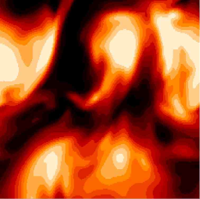
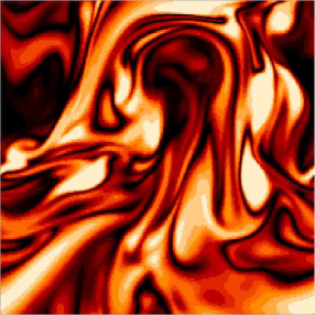
Figure 2: Cross sections of the absolute values of $\mathbf{u}$ (left panel) and $\mathbf{B}$ (right panel) in the saturated state of a simulation with ${Re}\simeq 100$, ${Pr}_{m}=10$ (run B of Ref. SCTMM_stokes ).

3 Isotropic MHD turbulence

Let us now consider the case of isotropic MHD turbulence, i.e., a turbulent plasma where no mean field is imposed externally. Can the scaling theories reviewed above be adapted to this case? A popular view, due originally to Kraichnan Kraichnan , is that everything remains the same with the role of the mean field $\mathbf{B}_{0}$ now played by the magnetic fluctuations at the outer scale, $\delta B_{L}$, while at smaller scales, the turbulence is again a local (in scale) cascade of Alfvénic ($\delta u_{l}\sim\delta B_{l}$) fluctuations. This picture is only plausible if the magnetic energy is dominated by the outer-scale fluctuations, an assumption that does not appear to hold in the numerical simulations of forced isotropic MHD turbulence SCTMM_stokes . Instead, the magnetic energy is concentrated at small scales, where the magnetic fluctuations significantly exceed the velocity fluctuations, with no sign of the scale-by-scale equipartition implied for an Alfvénic cascade. These features are especially pronounced when the magnetic Prandtl number ${Pr}_{m}=\nu/\eta={R}_{m}/{Re}\gg 1$, i.e., when the magnetic cutoff scale lies below the viscous cutoff of the velocity fluctuations (Fig. 2). The numerically more accessible case of ${Pr}_{m}\gtrsim 1$, while non-asymptotic and, therefore, harder to interpret, retains most of the features of the large-${Pr}_{m}$ regime. A handy formula for ${Pr}_{m}$ based on the Spitzer Spitzer_book values of $\nu$ and $\eta$ for fully ionised plasmas is

$${Pr}_{m}\sim 10^{-5}T^{4}/n,$$ (35)

where $T$ is the temperature in Kelvin and $n$ the particle density in cm^-3. Eq. (35) tends to give very large values for hot diffuse astrophysical plasmas: e.g., $10^{11}$ for the warm interstellar medium, $10^{29}$ for galaxy clusters.

Let us examine the situation in more detail. In the absence of a mean field, all magnetic fields are generated and maintained by the turbulence itself, i.e., isotropic MHD turbulence is the saturated state of the turbulent (small-scale) dynamo. Therefore, we start by considering how a weak (dynamically unimportant) magnetic field is amplified by turbulence in a large-${Pr}_{m}$ MHD fluid and what kind of field can be produced this way.

3.1 Small-scale dynamo

Many specific deterministic flows have been studied numerically and analytically and shown to be dynamos Childress_Gilbert . While rigourously determining whether any given flow is a dynamo is virtually always a formidable mathematical challenge, the combination of numerical and analytical experience of the last fifty years suggests that smooth three-dimensional flows with chaotic trajectories tend to have the dynamo property provided the magnetic Reynolds number exceeds a certain threshold, ${R}_{m}>{R}_{m,c}\sim 10^{1}...10^{2}$. In particular, the ability of Kolmogorov turbulence to amplify magnetic fields is a solid numerical fact first established by Meneguzzi et al. in 1981 Meneguzzi_Frisch_Pouquet and since then confirmed in many numerical studies with ever-increasing resolutions (most recently SCTMM_stokes ; Haugen_Brandenburg_Dobler ). It was, in fact, Batchelor who realised already in 1950 Batchelor that the growth of magnetic fluctuations in a random flow should occur simply as a consequence of the random stretching of the field lines and that it should proceed at the rate of strain associated with the flow. In Kolmogorov turbulence, the largest rate of strain $\sim\delta u_{l}/l$ is associated with the smallest scale $l\sim{l}_{\nu}$ — the viscous scale, so it is the viscous-scale motions that dominantly amplify the field (at large ${Pr}_{m}$). Note that the velocity field at the viscous scale is random but smooth, so the small-scale dynamo in Kolmogorov turbulence belongs to the same class as fast dynamos in smooth single-scale flows Childress_Gilbert ; SCTMM_stokes .

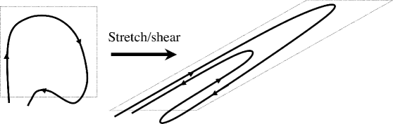
Figure 3: Stretching/shearing a magnetic-field line.

A repeated application of random stretching/shearing to a tangled magnetic field produces direction reversals at arbitrarily small scales, giving rise to a folded field structure (Fig. 3). It is an essential property of this structure that the strength of the field and the curvature of the field lines are anticorrelated: wherever the field is growing it is relatively straight (i.e., curved only on the scale of the flow), whereas in the bending regions, where the curvature is large, the field is weak. A quantitative theory of the folded structure can be constructed based on the joint statistics of the field strength $B=|\mathbf{B}|$ and curvature $\mathbf{K}=\hat{\mathbf{b}}\cdot\boldsymbol{\nabla}\hat{\mathbf{b}}$, where $\hat{\mathbf{b}}=\mathbf{B}/B$ SCMM_folding . The curvature is a quantity easily measured in numerical simulations, which confirm the overall straightness of the field and the curvature–field-strength anticorrelation SCTMM_stokes . At the end of this section, we shall give a simple demonstration of the validity of the folded structure.

The scale of the direction reversals is limited from below only by Ohmic diffusion: for Kolmogorov turbulence, balancing the rate of strain at the viscous scale with diffusion and taking ${Pr}_{m}\gg 1$ gives the resistive cutoff ${l}_{\eta}$:

$$\delta u_{{l}_{\nu}}/{l}_{\nu}\sim\eta/{l}_{\eta}^{2}\quad\Rightarrow\quad{l}_{\eta}\sim{Pr}_{m}^{-1/2}{l}_{\nu}.$$ (36)

If random stretching gives rise to magnetic fields with reversals at the resistive scale, why are these fields not eliminated by diffusion? In other words, how is the small-scale dynamo possible? It turns out that, in 3D, there are magnetic-field configurations that can be stretched without being destroyed by the concurrent refinement of the reversal scale and that add up to give rise to exponential growth of the magnetic energy. Below we give an analytical demonstration of this. It is a (somewhat modified) version of an ingenious argument originally proposed by Zeldovich et al. in 1984 Zeldovich_etal_linear . A reader looking solely for a broad qualitative picture of isotropic MHD turbulence may skip to § 3.2.

Figure 4: Ya. B. Zeldovich (1914-1987) (photo courtesy of M. Ya. Ovchinnikova).

Overcoming diffusion. Let us study magnetic fields with reversals at subviscous scales: at these scales, the velocity field is smooth and can, therefore, be expanded

$$u^{i}(t,\mathbf{x})=u^{i}(t,{\bf 0})+\sigma^{i}_{m}(t)x^{m}+\dots,$$ (37)

where $\sigma^{i}_{m}(t)$ is the rate-of-strain tensor. The expansion is around some reference point $\mathbf{x}={\bf 0}$. We can always go to the reference frame that moves with the velocity at this point, so that $u^{i}(t,{\bf 0})=0$. Let us seek the solution to Eq. (2) with velocity (37) as a sum of random plane waves with time-dependent wave vectors:

$$B^{i}(t,\mathbf{x})=\int{d^{3}k_{0}\over(2\pi)^{3}}\,\tilde{B}^{i}(t,\mathbf{k}_{0})e^{i\tilde{\mathbf{k}}(t,\mathbf{k}_{0})\cdot\mathbf{x}},$$ (38)

where $\tilde{\mathbf{k}}(0,\mathbf{k}_{0})=\mathbf{k}_{0}$, so $\tilde{B}^{i}(0,\mathbf{k}_{0})=B_{0}^{i}(\mathbf{k}_{0})$ is the Fourier transform of the initial field. Since Eq. (2) is linear, it is sufficient to ensure that each of the plane waves is individually a solution. This leads to two ordinary differential equations for every $\mathbf{k}_{0}$:

$$\partial_{t}\tilde{B}^{i}=\sigma^{i}_{m}\tilde{B}^{m}-\eta\tilde{k}^{2}\tilde{B}^{i},\qquad\partial_{t}\tilde{k}_{l}=-\sigma^{i}_{l}\tilde{k}_{i},$$ (39)

subject to initial conditions $\tilde{B}^{i}(0,\mathbf{k}_{0})=B^{i}_{0}(\mathbf{k}_{0})$ and $\tilde{k}_{l}(0,\mathbf{k}_{0})=k_{0l}$. The solution of these equations can be written explicitly in terms of the Lagragian transformation of variables $\mathbf{x}_{0}\to\mathbf{x}(t,\mathbf{x}_{0})$, where

$$\partial_{t}x^{i}(t,\mathbf{x}_{0})=u^{i}(t,\mathbf{x}(t,\mathbf{x}_{0}))=\sigma^{i}_{m}(t)x^{m}(t,\mathbf{x}_{0}),\qquad x^{i}(0,\mathbf{x}_{0})=x^{i}_{0}.$$ (40)

Because of the linearity of the velocity field, the strain tensor $\partial x^{i}/\partial x_{0}^{m}$ and its inverse $\partial x_{0}^{r}/\partial x^{l}$ are functions of time only. At $t=0$, they are unit matrices. At $t>0$, they satisfy

$$\partial_{t}{\partial x^{i}\over\partial x_{0}^{m}}=\sigma^{i}_{l}{\partial x^{l}\over\partial x_{0}^{m}},\qquad\partial_{t}{\partial x_{0}^{r}\over\partial x^{l}}=-\sigma^{i}_{l}{\partial x^{r}\over\partial x_{0}^{i}}.$$ (41)

We can check by direct substitution that

$$\tilde{B}^{i}(t,\mathbf{k}_{0})={\partial x^{i}\over\partial x_{0}^{m}}\,B_{0}^{m}(\mathbf{k}_{0})\exp\left[-\eta\int_{0}^{t}dt^{\prime}\tilde{k}^{2}(t^{\prime})\right],\quad\tilde{k}_{l}(t,\mathbf{k}_{0})={\partial x_{0}^{r}\over\partial x^{l}}\,k_{0r}.$$ (42)

These formulae express the evolution of one mode in the integral (38). Using the fact that $\det(\partial x_{0}^{r}/\partial x^{l})=1$ in an incompressible flow and that Eq. (42) therefore establishes a one-to-one correspondence $\mathbf{k}\leftrightarrow\mathbf{k}_{0}$, it is easy to prove that the volume-integrated magnetic energy is the sum of the energies of individual modes:

$$\langle B^{2}\rangle(t)\equiv\int d^{3}x\,|\mathbf{B}(t,\mathbf{x})|^{2}=\int{d^{3}k_{0}\over(2\pi)^{3}}\,|\tilde{\mathbf{B}}(t,\mathbf{k}_{0})|^{2}.$$ (43)

From Eq. (42),

$$|\tilde{\mathbf{B}}(t,\mathbf{k}_{0})|^{2}=\mathbf{B}_{0}(\mathbf{k}_{0})\cdot\hat{\mathsf{M}}(t)\cdot\mathbf{B}_{0}^{*}(\mathbf{k}_{0})\exp\left[-2\eta\int_{0}^{t}dt^{\prime}\,\mathbf{k}_{0}\cdot\hat{\mathsf{M}}^{-1}(t^{\prime})\cdot\mathbf{k}_{0}\right],$$ (44)

where the matrices $\hat{\mathsf{M}}$ and $\hat{\mathsf{M}}^{-1}$ have elements defined by

$$M_{mn}(t)={\partial x^{i}\over\partial x_{0}^{m}}{\partial x^{i}\over\partial x_{0}^{n}}\quad\mathrm{and}\quad M^{rs}(t)={\partial x_{0}^{r}\over\partial x^{l}}{\partial x_{0}^{s}\over\partial x^{l}},$$ (45)

respectively. They are the co- and contravariant metric tensors of the inverse Lagrangian transformation $\mathbf{x}\to\mathbf{x}_{0}$.

Let us consider the simplest possible case of a flow (37) with constant $\hat{\sigma}=\mathrm{diag}\left\{\lambda_{1},\lambda_{2},\lambda_{3}\right\}$, where $\lambda_{1}>\lambda_{2}\geq 0>\lambda_{3}$ and $\lambda_{1}+\lambda_{2}+\lambda_{3}=0$ by incompressibility. Then $\hat{\mathsf{M}}=\mathrm{diag}\left\{e^{2\lambda_{1}t},e^{2\lambda_{2}t},e^{2\lambda_{3}t}\right\}$ and Eq. (44) becomes, in the limit $t\to\infty$,

$$|\tilde{\mathbf{B}}(t,\mathbf{k}_{0})|^{2}\sim|B_{0}^{1}(\mathbf{k}_{0})|^{2}\exp\left[2\lambda_{1}t-\eta\left({k_{01}^{2}\over\lambda_{1}}+{k_{02}^{2}\over\lambda_{2}}+{k_{03}^{2}\over|\lambda_{3}|}\,e^{2|\lambda_{3}|t}\right)\right],$$ (46)

where we have dropped terms that decay exponentially with time compared to those retained. We see that for most $\mathbf{k}_{0}$, the corresponding modes decay superexponentially fast with time. The domain in the $\mathbf{k}_{0}$ space containing modes that are not exponentially small at any given time $t$ is given by

$${k_{01}^{2}\over\lambda_{1}^{2}t/\eta}+{k_{02}^{2}\over\lambda_{1}\lambda_{2}t/\eta}+{k_{03}^{2}\over\lambda_{1}|\lambda_{3}|te^{2\lambda_{3}t}/\eta}<\mathrm{const}.$$ (47)

The volume of this domain at time $t$ is $\sim\lambda_{1}^{2}(\lambda_{2}|\lambda_{3}|)^{1/2}(t/\eta)^{3/2}e^{\lambda_{3}t}$. Within this volume, $|\tilde{\mathbf{B}}(t,\mathbf{k}_{0})|^{2}\sim|B_{0}^{1}(\mathbf{k}_{0})|^{2}e^{2\lambda_{1}t}$. Using $\lambda_{3}=-\lambda_{1}-\lambda_{2}$ and Eq. (43), we get

$$\langle B^{2}\rangle(t)\propto\exp\left[(\lambda_{1}-\lambda_{2})t\right].$$ (48)

Let us discuss the physics behind the Zeldovich et al. calculation sketched above. When the magnetic field is stretched by the flow, it naturally aligns with the stretching Lyapunov direction: $\mathbf{B}\sim\hat{\mathbf{e}}_{1}B_{0}^{1}e^{\lambda_{1}t}$. The wave vector $\mathbf{k}$ has a tendency to align with the compression direction: $\mathbf{k}\sim\hat{\mathbf{e}}_{3}k_{03}e^{|\lambda_{3}|t}$, which makes most modes decay superexponentially. The only ones that survive are those whose $\mathbf{k}_{0}$’s were nearly perpendicular to $\hat{\mathbf{e}}_{3}$, with the permitted angular deviation from $90^{\circ}$ decaying exponentially in time $\sim e^{-|\lambda_{3}|t}$. Since the magnetic field is solenoidal, $\mathbf{B}_{0}\perp\mathbf{k}_{0}$, the modes that get stretched the most have $\mathbf{B}_{0}\parallel\hat{\mathbf{e}}_{1}$ and $\mathbf{k}_{0}\parallel\hat{\mathbf{e}}_{2}$ (Fig. 5). In contrast, in 2D, the field aligns with $\hat{\mathbf{e}}_{1}$ and must, therefore, reverse along $\hat{\mathbf{e}}_{2}$, which is always the compression direction (Fig. 5), so the stretching is always overwhelmed by the diffusion and no dynamo is possible (as should be the case according to the rigourous early result of Zeldovich Zeldovich_antidynamo ).

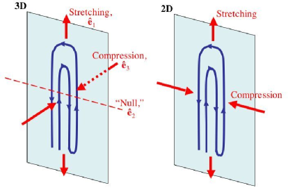
Figure 5: Magnetic fields vs. the Lyapunov directions (from SCTMM_stokes ). Zeldovich et al. Zeldovich_etal_linear did not give this exact interpretation of their calculation because the folded structure of the field was not yet clearly understood at the time.

The above construction can be generalised to time-dependent and random velocity fields. The matrix $\hat{\mathsf{M}}$ is symmetric and can, therefore, be diagonalised by an appropriate rotation $\hat{\mathsf{R}}$ of the coordinate system: $\hat{\mathsf{M}}=\hat{\mathsf{R}}^{T}\cdot\hat{\mathsf{L}}\cdot\hat{\mathsf{R}}$, where, by definition, $\hat{\mathsf{L}}=\mathrm{diag}\left\{e^{\zeta_{1}(t)},e^{\zeta_{2}(t)},e^{\zeta_{3}(t)}\right\}$. It is possible to prove that, as $t\to\infty$, $\hat{\mathsf{R}}(t)\to\left\{\hat{\mathbf{e}}_{1},\hat{\mathbf{e}}_{2},\hat{\mathbf{e}}_{3}\right\}$ and $\zeta_{i}(t)/2t\to\lambda_{i}$, where $\hat{\mathbf{e}}_{i}$ are constant orthogonal unit vectors, which make up the Lyapunov basis, and $\lambda_{i}$ are the Lyapunov exponents of the flow Goldhirsch_Sulem_Orszag . The instantaneous values of $\zeta_{i}(t)/2t$ are called finite-time Lyapunov exponents. For a random flow, $\zeta_{i}(t)$ are random functions. Eq. (48) generalises to

$$\langle\overline{B^{2}}\rangle(t)\propto\overline{\exp\left[(\zeta_{1}-\zeta_{2})/2\right]},$$ (49)

where the overline means averaging over the distribution of $\zeta_{i}$. The only random flow for which this distribution is known is a Gaussian white-in-time velocity first considered in the dynamo context in 1967 by Kazantsev Kazantsev . The distribution of $\zeta_{i}$ for this flow is Gaussian in the long-time limit and Eq. (49) gives $\langle B^{2}\rangle\propto e^{(5/4)\lambda_{1}t}$, where $\lambda_{1}=\langle\zeta_{1}\rangle/2t$ Chertkov_etal_dynamo . For Kazantsev’s velocity, it is also possible to calculate the magnetic-energy spectrum Kazantsev ; Kulsrud_Anderson , which is the spectrum of the direction reversals. It has a peak at the resistive scale and a $k^{+3/2}$ power law stretching across the subviscous range, ${l}_{\nu}^{-1}\ll k\ll{l}_{\eta}^{-1}$. This scaling appears to be corroborated by numerical simulations SCTMM_stokes ; Haugen_Brandenburg_Dobler .

Folded structure revisited. We shall now give a very simple demonstration that linear stretching does indeed produce folded fields with straight/curved field lines corresponding to larger/smaller field strength. Using Eq. (2), we can write evolution equations for the field strength $B=|\mathbf{B}|$, the field direction $\hat{\mathbf{b}}=\mathbf{B}/B$ and the field-line curvature $\mathbf{K}=\hat{\mathbf{b}}\cdot\boldsymbol{\nabla}\hat{\mathbf{b}}$. Omitting the resistive terms,

$${dB\over dt} = \bigl{(}\hat{\mathbf{b}}\hat{\mathbf{b}}:\boldsymbol{\nabla}\mathbf{u}\bigr{)}B,$$ (50)

$${d\hat{\mathbf{b}}\over dt} = \hat{\mathbf{b}}\cdot\bigl{(}\boldsymbol{\nabla}\mathbf{u}\bigr{)}\cdot\bigl{(}\hat{\mathsf{I}}-\hat{\mathbf{b}}\hat{\mathbf{b}}\bigr{)},$$ (51)

$${d\mathbf{K}\over dt} = \mathbf{K}\cdot\bigl{(}\boldsymbol{\nabla}\mathbf{u}\bigr{)}\cdot\bigl{(}\hat{\mathsf{I}}-\hat{\mathbf{b}}\hat{\mathbf{b}}\bigr{)}-2(\hat{\mathbf{b}}\hat{\mathbf{b}}:\boldsymbol{\nabla}\mathbf{u})\mathbf{K}-\bigl{[}\hat{\mathbf{b}}\cdot\bigl{(}\boldsymbol{\nabla}\mathbf{u}\bigr{)}\cdot\mathbf{K}\bigr{]}\hat{\mathbf{b}}$$ (52)

$$+\hat{\mathbf{b}}\hat{\mathbf{b}}:\bigl{(}\boldsymbol{\nabla}\boldsymbol{\nabla}\mathbf{u}\bigr{)}\cdot\bigl{(}\hat{\mathsf{I}}-\hat{\mathbf{b}}\hat{\mathbf{b}}\bigr{)}.$$

For simplicity, we again use the velocity field (37) with constant $\hat{\sigma}=\mathrm{diag}\left\{\lambda_{1},\lambda_{2},\lambda_{3}\right\}$. Then the stable fixed point of Eq. (51) in the comoving frame is $\hat{\mathbf{b}}=\hat{\mathbf{e}}_{1}$ (magnetic field aligns with the principal stretching direction), whence $B\propto e^{\lambda_{1}t}$. Since $\mathbf{K}\cdot\hat{\mathbf{b}}=0$, we set $K_{1}=0$. Denoting $\boldsymbol{\Sigma}=\hat{\mathbf{b}}\hat{\mathbf{b}}:\boldsymbol{\nabla}\boldsymbol{\nabla}\mathbf{u}$, we can now write Eq. (52) as

$${dK_{2}\over dt}=-\bigl{(}2\lambda_{1}-\lambda_{2}\bigr{)}K_{2}+\Sigma_{2},\qquad{dK_{3}\over dt}=-\bigl{(}3\lambda_{1}+\lambda_{2}\bigr{)}K_{3}+\Sigma_{3}.$$ (53)

Both components of $\mathbf{K}$ decay exponentially, until they are comparable to the inverse scale of the velocity field (i.e., the terms containing $\boldsymbol{\nabla}\boldsymbol{\nabla}\mathbf{u}$ become important). The stationary solution is $K_{2}=\Sigma_{2}/(2\lambda_{1}-\lambda_{2})$, $K_{3}=\Sigma_{3}/(3\lambda_{1}+\lambda_{2})$.

If the field is to reverse direction, it must turn somewhere (see Fig. 3). At such a turning point, the field must be perpendicular to the stretching direction. Setting $b_{1}=0$, we find two fixed points of Eq. (51) under this condition: $\hat{\mathbf{b}}=\hat{\mathbf{e}}_{2}$ and $\hat{\mathbf{b}}=\hat{\mathbf{e}}_{3}$. Only the former is stable, so the field at the turning point will tend to align with the “null” direction. Thus, stretching favours configurations with field reversals along the “null” direction, which are also those that survive diffusion (see Fig. 5). From Eq. (52) we find that at the turning point, $K_{2}=0$, $K_{3}=\Sigma_{3}/(\lambda_{1}+3\lambda_{2})$, while $K_{1}$ grows at the rate $\lambda_{1}-2\lambda_{2}$ (assumed positive). This growth continues until limited by diffusion at $K\sim 1/{l}_{\eta}$. The strength of the field in this curved region is $\propto e^{\lambda_{2}t}$, so the fields are weaker than in the straight segments, where $B\propto e^{\lambda_{1}t}$.

When the problem is solved for the Kazantsev velocity, the above solution generalises to a field of random curvatures anticorrelated with the magnetic-field strength and with a stationary PDF of $K$ that has a peak at $K\sim\mathrm{flow\ scale}^{-1}$ and a power tail $\sim K^{-13/7}$ describing the distribution of curvatures at the turning points SCMM_folding . Numerical simulations support these results SCTMM_stokes .

G. K. Batchelor (1920-2000)		A. Schlüter		L. Biermann (1907-1986)

Figure 6: Photo of A. Schlüter courtesy of MPI für Plasmaphysik; photo of L. Biermann courtesy of Max-Planck-Gesellschaft/AIP Emilio Segrè Visual Archives.

3.2 Saturation of the dynamo

The small-scale dynamo gave us exponentially growing magnetic fields with energy concentrated at small (resistive) scales. How is the growth of magnetic energy saturated and what is the final state? Will magnetic energy stay at small scales or will it proceed to scale-by-scale equipartition via some form of inverse cascade? This basic dichotomy dates back to the 1950 papers by Batchelor Batchelor and Schlüter & Biermann Schlueter_Biermann . Batchelor thought that magnetic field was basically analogous to the vorticity field $\boldsymbol{\omega}=\boldsymbol{\nabla}\times\mathbf{u}$ (which satisfies the same equation (2) except for the difference between $\eta$ and $\nu$) and would, therefore, saturate at a low energy, $\langle B^{2}\rangle\sim{Re}^{-1/2}\langle u^{2}\rangle$, with a spectrum peaked at the viscous scale. Schlüter and Biermann disagreed and argued that the saturated state would be a scale-by-scale balance between the Lorentz and inertial forces, with turbulent motions at each scale giving rise to magnetic fluctuations of matching energy at the same scale. Schlüter and Biermann’s argument (and, implicitly, also Batchelor’s) was based on the assumption of locality of interaction (in scale space) between the magnetic and velocity fields: locality both of the dynamo action and of the back reaction. As we saw in the previous section, this assumption is certainly incorrect for the dynamo: a linear velocity field, i.e., a velocity field of a formally infinitely large (in practice, viscous) scale can produce magnetic fields with reversals at the smallest scale allowed by diffusion. A key implication of the folded structure of these fields concerns the Lorentz force, the essential part of which, in the case of incompressible flow, is the curvature force $B^{2}\mathbf{K}$. Since it is a quantity that depends only on the parallel gradient of the magnetic field and does not know about direction reversals, it will possess a degree of velocity-scale spatial coherence necessary to oppose stretching. Thus, a field that is formally at the resistive scale will exert a back reaction at the scale of the velocity field. In other words, interactions are nonlocal: a random flow at a given scale $l$, having amplified the magnetic fields at the resistive scale ${l}_{\eta}\ll l$, will see these magnetic fields back react at the scale $l$. Given the nonlocality of back reaction, we can update Batchelor’s and Schlüter & Biermann’s scenarios for saturation in the following way SCHMM_ssim ; SCTMM_stokes .

The magnetic energy is amplified by the viscous-scale motions until the field is strong enough to resist stretching, i.e., until $\mathbf{B}\cdot\boldsymbol{\nabla}\mathbf{B}\sim\mathbf{u}\cdot\boldsymbol{\nabla}\mathbf{u}\sim\delta u_{{l}_{\nu}}^{2}/{l}_{\nu}$. Since $\mathbf{B}\cdot\boldsymbol{\nabla}\mathbf{B}\sim B^{2}K\sim B^{2}/{l}_{\nu}$ (folded field), this happens when

$$\langle B^{2}\rangle\sim\delta u_{{l}_{\nu}}^{2}\sim{Re}^{-1/2}\langle u^{2}\rangle.$$ (54)

Let us suppose that the viscous motions are suppressed by the back reaction, at least in their ability to amplify the field. Then the motions at larger scales in the inertial range come into play: while their rates of strain and, therefore, the associated stretching rates are smaller than that of the viscous-scale motions, they are more energetic [see Eq. (4)], so the magnetic field is too weak to resist being stretched by them. As the field continues to grow, it will suppress the motions at ever larger scales. If we define a stretching scale ${l}_{\mathrm{s}}(t)$ as the scale of the motions whose energy is $\delta u_{{l}_{\mathrm{s}}}\sim\langle B^{2}\rangle(t)$, we can estimate

$${d\over dt}\langle B^{2}\rangle\sim{\delta u_{{l}_{\mathrm{s}}}\over{l}_{\mathrm{s}}}\langle B^{2}\rangle\sim{\delta u_{{l}_{\mathrm{s}}}^{3}\over{l}_{\mathrm{s}}}\sim\epsilon=\mathrm{const}\quad\Rightarrow\quad\langle B^{2}\rangle(t)\sim\epsilon t.$$ (55)

Thus, exponential growth gives way to secular growth of the magnetic energy. This is accompanied by elongation of the folds (their length is always of the order of the stretching scale, ${l}_{\parallel}\sim{l}_{\mathrm{s}}$), while the resistive (reversal) scale increases because the stretching rate goes down:

$${l}_{\parallel}(t)\sim{l}_{\mathrm{s}}(t)\sim\delta u_{{l}_{\mathrm{s}}}^{3}/\epsilon\sim\sqrt{\epsilon}\,t^{3/2},\quad{l}_{\eta}(t)\sim\left[\eta/(\delta u_{{l}_{\mathrm{s}}}/{l}_{\mathrm{s}})\right]^{1/2}\sim\sqrt{\eta t}.$$ (56)

This secular stage can continue until the entire inertial range is suppressed, ${l}_{\mathrm{s}}\sim L$, at which point saturation must occur. This happens after $t\sim\epsilon^{-1/3}L^{2/3}\sim L/\delta u_{L}$. Using Eqs. (55)-(56), we have, in saturation,

$$\langle B^{2}\rangle\sim\langle u^{2}\rangle,\quad{l}_{\parallel}\sim L,\quad{l}_{\eta}\sim\left[\eta/(\delta u_{L}/L)\right]^{1/2}\sim{R}_{m}^{-1/2}L.$$ (57)

Comparing Eqs. (57) and (36), we see that the resistive scale has increased only by a factor of ${Re}^{1/4}$ over its value in the weak-field growth stage. Note that this imposes a very stringent requirement on any numerical experiment striving to distinguish between the viscous and resistive scales: ${Pr}_{m}\gg{Re}^{1/2}\gg 1$.

If, as in the above scenario, the magnetic field retains its folded structure in saturation, with direction reversals at the resistive scale, this explains qualitatively why the numerical simulations of the developed isotropic MHD turbulence with ${Pr}_{m}\geq 1$ SCTMM_stokes show the magnetic-energy pile-up at the small scales. What then is the saturated state of the turbulent velocity field? We assumed above that the inertial-range motions were “suppressed” — this applied to their ability to amplify magnetic field, but needed not imply a complete evacuation of the inertial range. Indeed, simulations at modest ${Pr}_{m}$ show a powerlike velocity spectrum SCTMM_stokes ; Haugen_Brandenburg_Dobler . The most obvious class of motions that can populate the inertial range without affecting the magnetic-field strength are a type of Alfvén waves that propagate not along a mean (or large-scale) magnetic field but along the folded structure (Fig. 7). Mathematically, the dispersion relation for such waves is derived via a linear theory carried out for the inertial-range perturbations ($L^{-1}\ll k\ll{l}_{\nu}^{-1}$) of the tensor $B_{i}B_{j}$ (cf. Gruzinov_Diamond96 ). The unperturbed state is the average of this tensor over the subviscous scales: $\langle B_{i}B_{j}\rangle=\hat{b}_{i}\hat{b}_{j}\langle B^{2}\rangle$, where $\langle B^{2}\rangle$ is the total magnetic energy and the tensor $\hat{b}_{i}\hat{b}_{j}$ only varies at the outer scale $L$ [Eq. (57)]. The resulting dispersion relation is $\omega=\pm|\mathbf{k}\cdot\hat{\mathbf{b}}|\langle B^{2}\rangle^{1/2}$ SCHMM_ssim . The presence of these waves will not change the resistive-scale-dominated nature of the magnetic-energy spectrum, but should be manifest in the kinetic-energy spectrum. There is, at present, no theory of a cascade of such waves, although a line of argument similar to § 2 might work, since it does not depend on the field having a specific direction. A numerical detection of these waves is also a challenge for the future.

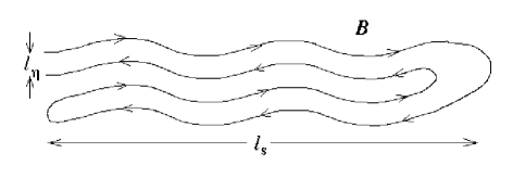
Figure 7: Alfvén waves propagating along folded fields (from SCHMM_ssim ).

What we have proposed above can be thought of as a modernised version of the Schlüter & Biermann scenario, retaining the intermediate secular-growth stage and saturation with $\langle B^{2}\rangle\sim\langle u^{2}\rangle$, but not scale-by-scale equipartition. However, an alternative possibility, which is in a similar relationship to Batchelor’s scenario, can also be envisioned. In Eqs. (55)-(56), the scale ${l}_{\eta}$ at which diffusion cuts off the small-scale magnetic fluctuations was assumed to be determined by the stretching rate $\delta u_{{l}_{\mathrm{s}}}/{l}_{\mathrm{s}}$. However, since the nonlinear suppression of the viscous-scale eddies only needs to eliminate motions with $\hat{\mathbf{b}}\hat{\mathbf{b}}:\boldsymbol{\nabla}\mathbf{u}\neq 0$ [Eq. (50)], two-dimensional “interchange” motions (velocity gradients $\perp\hat{\mathbf{b}}$) are, in principle, allowed to survive at the viscous scale. These could “two-dimensionally” mix the direction-reversing magnetic fields at the rate $\delta u_{{l}_{\nu}}/{l}_{\nu}$ — much faster than the unsuppressed larger-scale stretching can amplify the field, — with the consequence that the resistive scale is pinned at the value given by Eq. (36) and the field cannot grow above the Batchelor limit (54). The mixing efficiency of the suppressed motions is the key to choosing between the two saturation scenarios. Numerical simulations SCTMM_stokes corroborate the existence of an intermediate stage of slower-than-exponential growth accompanied by fold elongation and a modest increase of the resistive scale [Eq. (56)]. This tips the scales in favour of the first scenario, but, in view of limited resolutions, we hesitate to declare the matter definitively resolved.

3.3 Turbulence and magnetic fields in galaxy clusters

The intracluster medium (hereafter, ICM) is a hot ($T\sim 10^{8}$ K) diffuse ($n\sim 10^{-2}...10^{-3}$ cm^-3) fully ionised plasma, which accounts for most of the luminous matter in the Universe (note that it is not entirely dissimilar from the ionised phases of the interstellar medium: e.g., the so-called hot ISM). It is a natural astrophysical environment to which the large-${Pr}_{m}$ isotropic regime of MHD turbulence appears to be applicable: indeed, Eq. (35) gives ${Pr}_{m}\sim 10^{29}$.

The ICM is believed to be in a state of turbulence driven by a variety of mechanisms: merger events, galactic and subcluster wakes, active galactic nuclei. One expects the outer scale $L\sim 10^{2}...10^{3}$ kpc and the velocity dispersions $\delta u_{L}\sim 10^{2}...10^{3}$ km/s (a fraction of the sound speed). Indirect observational evidence supporting the possibility of a turbulent ICM with roughly these parameters already exists (an apparently powerlike spectrum of pressure fluctuations found in the Coma cluster Schuecker_etal , broadened abundance profiles in Perseus believed to be caused by turbulent diffusion Rebusco_etal ), and direct detection may be achieved in the near future Inogamov_Sunyaev . However, there is as yet no consensus on whether turbulence, at least in the usual hydrodynamic sense, is a generic feature of clusters Fabian_etal_Perseus2 . The main difficulty is the very large values of the ICM viscosity obtained via the standard estimate $\nu\sim{v}_{\mathrm{th},i}{\lambda}_{\mathrm{mfp}}$, where ${v}_{\mathrm{th},i}\sim 10^{3}$ km/s is the ion thermal speed and ${\lambda}_{\mathrm{mfp}}\sim 1...10$ kpc is the ion mean free path. This gives ${Re}\sim 10^{2}$ if not less, which makes the existence of a well-developed inertial range problematic. Postponing the problem of viscosity until § 4, we observe that the small-scale dynamo does not, in fact, require a turbulent velocity field in the sense of a broad inertial range: in the weak-field regime discussed in § 3.1, the dynamo was controlled by the smooth single-scale random flow associated with the viscous-scale motions; in saturation, we argued in § 3.2 that the main effect was the direct nonlocal interaction between the outer-scale (random) motions and the magnetic field. Given the available menu of large-scale stirring mechanisms in clusters, it is likely that, whatever the value of ${Re}$, the velocity field is random.

The cluster turbulence is certainly magnetic. The presence of magnetic fields was first demonstrated for the Coma cluster, for which Willson detected in 1970 a diffuse synchrotron radio emission Willson and Kim et al. in 1990 were able to estimate directly the magnetic-field strength and scale using the Faraday rotation measure (RM) data Kim_etal_Coma . Such observations of magnetic fields in clusters have now become a vibrant area of astronomy (reviewed most recently in Govoni_Feretti_review ), usually reporting a field $B\sim 1...10\ \mu$G at scales $\sim 1...10$ kpc Clarke_Kronberg_Boehringer . All of this field is small-scale fluctuations: no appreciable mean component has been detected. The field is dynamically significant: the magnetic energy is less but not much less than the kinetic energy of the turbulent motions.

Do clusters fit the theoretical expectations reviewed above? The magnetic-field scale seen in clusters is usually 10 to 100 times smaller than the expected outer scale of turbulent motions and, indeed, is also smaller than the viscous scale based on ${Re}\sim 10^{2}$. However, it is certainly far above the resistive scale, which turns out be ${l}_{\eta}\sim 10^{3}...10^{4}$ km! Faced with these numbers, we must suspend the discussion of cluster physics and finally take account of the fact that astrophysical bodies are made of plasma, not of an MHD fluid.

4 Enter plasma physics

4.1 Braginskii viscosity

In all of the above, we have used the MHD equations (1) and (2) to develop turbulence theories supposed to be relevant for astrophysical plasmas. Historically, such has been the approach followed in most of the astrophysical literature. The philosophy underpinning this approach is again that of universality: the “microphysics” at and below the dissipation scale are not expected to matter for the fluid-like dynamics at larger scales. However, in considering the MHD turbulence with large ${Pr}_{m}$, we saw that dissipation scales, determined by the values of the viscosity $\nu$ and magnetic diffusivity $\eta$, played a very prominent role: the growth of the small-scale magnetic fields was controlled by the turbulent rate of strain at the viscous scale and resulted in the magnetic energy piling up, in the form of direction-reversing folded fields, at the resistive scale — both in the growth and saturation stages of the dynamo. It is then natural to revisit the question of whether the Laplacian diffusion terms in Eqs. (1)-(2) are a good description of the dissipation in astrophysical plasmas.

The answer to this question is, of course, that they are not. A necessary assumption in the derivation of these terms is that the ion cyclotron frequency $\Omega_{i}=eB/m_{i}c$ exceeds the ion-ion collision frequency ${\nu}_{ii}$ or, equivalently, the ion gyroradius $\rho_{i}={v}_{\mathrm{th},i}/\Omega_{i}$ exceeds the mean free path ${\lambda}_{\mathrm{mfp}}={v}_{\mathrm{th},i}/{\nu}_{ii}$. This is patently not the case in many astrophysical plasmas: for example, in galaxy clusters, ${\lambda}_{\mathrm{mfp}}\sim 1...10$ kpc, while $\rho_{i}\sim 10^{4}$ km. In such a weakly collisional magnetised plasma, the momentum equation (1) assumes the following form, valid at spatial scales $\gg\rho_{i}$ and at time scales $\gg\Omega_{i}^{-1}$,

$${d\mathbf{u}\over dt}=-\boldsymbol{\nabla}\left({p}_{\perp}+{B^{2}\over 2}\right)+\boldsymbol{\nabla}\cdot\bigl{[}\hat{\mathbf{b}}\hat{\mathbf{b}}({p}_{\perp}-{p}_{\parallel}+B^{2})\bigr{]}+\mathbf{f},$$ (58)

where ${p}_{\perp}$ and ${p}_{\parallel}$ are plasma pressures perpendicular and parallel to the local direction of the magnetic field, respectively, and we have used $\mathbf{B}\cdot\boldsymbol{\nabla}\mathbf{B}=\boldsymbol{\nabla}\cdot(\hat{\mathbf{b}}\hat{\mathbf{b}}B^{2})$. The evolution of the magnetic field is controlled by the electrons — the field remains frozen into the flow and we may use Eq. (2) with $\eta=0$.

If we are interested in subsonic motions, $\boldsymbol{\nabla}({p}_{\perp}+B^{2}/2)$ in Eq. (58) can be found from the incompressibility condition $\boldsymbol{\nabla}\cdot\mathbf{u}=0$ and the only quantity still to be determined is ${p}_{\perp}-{p}_{\parallel}$. The proper way to compute it is by a rather lengthy kinetic calculation due to Braginskii Braginskii , which cannot be repeated here. The result of this calculation can, however, be obtained in the following heuristic way SCKHS_brag .

The fundamental property of charged particles moving in a magnetic field is the conservation of the first adiabatic invariant $\mu=m_{i}{v}_{\perp}^{2}/2B$. When ${\lambda}_{\mathrm{mfp}}\gg\rho_{i}$, this conservation is only weakly broken by collisions. As long as $\mu$ is conserved, any change in $B$ must be accompanied by a proportional change in ${p}_{\perp}$. Thus, the emergence of the pressure anisotropy is a natural consequence of the changes in the magnetic-field strength and vice versa: indeed, summing up the first adiabatic invariants of all particles, we get ${p}_{\perp}/B=\mathrm{const}$. Then

$${1\over{p}_{\perp}}{d{p}_{\perp}\over dt}={1\over B}{dB\over dt}-{\nu}_{ii}\,{{p}_{\perp}-{p}_{\parallel}\over{p}_{\perp}},$$ (59)

where the second term on the right-hand sight represents the collisional relaxation of the pressure anisotropy ${p}_{\perp}-{p}_{\parallel}$ at the rate ${\nu}_{ii}\sim{v}_{\mathrm{th},i}/{\lambda}_{\mathrm{mfp}}$. Using Eq. (50) for $B$ and balancing the terms in the rhs of Eq. (59), we get

$${p}_{\perp}-{p}_{\parallel}={\nu}_{\parallel}\,{1\over B}{dB\over dt}={\nu}_{\parallel}\hat{\mathbf{b}}\hat{\mathbf{b}}:\boldsymbol{\nabla}\mathbf{u},$$ (60)

where ${\nu}_{\parallel}\sim p/{\nu}_{ii}\sim{v}_{\mathrm{th},i}{\lambda}_{\mathrm{mfp}}$ is the “parallel viscosity.” This equation turns out to be exact Braginskii up to numerical prefactors in the definition of ${\nu}_{\parallel}$.

The energy conservation law based on Eqs. (58) and (2) is

$${d\over dt}\left({\langle u^{2}\rangle\over 2}+{\langle B^{2}\rangle\over 2}\right)=\epsilon-{\nu}_{\parallel}\bigl{<}|\hat{\mathbf{b}}\hat{\mathbf{b}}:\boldsymbol{\nabla}\mathbf{u}|^{2}\bigr{>}=\epsilon-{\nu}_{\parallel}\left<\left({1\over B}{dB\over dt}\right)^{2}\right>,$$ (61)

where Ohmic diffusion has been omitted. Thus, the Braginskii viscosity only dissipates such velocity gradients that change the strength of the magnetic field. The motions that do not affect $B$ are allowed to exist in the subviscous scale range. In the weak-field regime, these motions take the form of plasma instabilities. When the magnetic field is strong, a cascade of shear-Alfvén waves can be set up below the viscous scale. Let us elaborate.

4.2 Plasma instabilities

The simplest way to see that the pressure anisotropy in Eq. (58) leads to instabilities is as follows SCKHS_brag . Imagine a “fluid” solution with $\mathbf{u}$, ${p}_{\perp}$, ${p}_{\parallel}$, $\mathbf{B}$ changing on viscous time and spatial scales, $t\sim|\boldsymbol{\nabla}\mathbf{u}|^{-1}\sim{l}_{\nu}/\delta u_{{l}_{\nu}}$ and $l\sim{l}_{\nu}$. Would such a solution be stable with respect to fast ($\omega\gg|\boldsymbol{\nabla}\mathbf{u}|^{-1}$) small-scale ($k\gg{l}_{\nu}^{-1}$) perturbations? Linearising Eq. (58) and denoting perturbations by $\delta$, we get

$$-i\omega\delta\mathbf{u} = -i\mathbf{k}\left(\delta{p}_{\perp}+B\delta B\right)+\left({p}_{\perp}-{p}_{\parallel}+B^{2}\right)\delta\mathbf{K}$$ (62)

$$+\,\,i\hat{\mathbf{b}}\,{k}_{\parallel}\left[\delta{p}_{\perp}-\delta{p}_{\parallel}-\left({p}_{\perp}-{p}_{\parallel}-B^{2}\right){\delta B/B}\right],$$

where the perturbation of the field curvature is $\delta\mathbf{K}={k}_{\parallel}^{2}\delta\mathbf{u}_{\perp}/i\omega$ [see Eq. (52)]. We see that regardless of the origin of the pressure anisotropy, the shear-Alfvén-polarised perturbations ($\delta\mathbf{u}\propto\mathbf{k}\times\hat{\mathbf{b}}$) have the dispersion relation

$$\omega=\pm{k}_{\parallel}\left({p}_{\perp}-{p}_{\parallel}+B^{2}\right)^{1/2}.$$ (63)

When ${p}_{\parallel}-{p}_{\perp}>B^{2}$, $\omega$ is purely imaginary and we have what is known as the firehose instability Rosenbluth ; Chandrasekhar_Kaufman_Watson ; Parker_firehose ; Vedenov_Sagdeev . The growth rate of the instability is $\propto{k}_{\parallel}$, which means that the fastest-growing perturbations will be at scales far below the viscous scale or, indeed, the mean free path. Therefore, adopting the Braginskii viscosity [Eq. (60)] exposes a fundamental problem with the use of the MHD approximation for fully ionised plasmas: the equations are ill posed wherever ${p}_{\parallel}-{p}_{\perp}>B^{2}$. To take into account the instability and its impact on the large-scale dynamics, the fluid equations must be abandoned and a kinetic description adopted. A linear kinetic calculation shows that the instability growth rate peaks at ${k}_{\parallel}\rho_{i}\sim 1$, so the fluctuations grow fastest at the ion gyroscale. While the firehose instability occurs in regions where the velocity field leads to a decrease in the magnetic-field strength [Eq. (60)], a kinetic calculation of the pressure perturbations in Eq. (62) shows that another instability, called the mirror mode Parker_firehose , is triggered wherever the field increases (${p}_{\perp}>{p}_{\parallel}$). Its growth rate is also $\propto{k}_{\parallel}$ and peaks at the ion gyroscale.

In weakly collisional astrophysical plasmas such as the ICM, the random motions produced by the large-scale stirring will stretch and fold magnetic fields, giving rise to regions both of increasing and decreasing field strength (§ 3.1). The instabilities should, therefore, be present in weak-field regions where $|{p}_{\parallel}-{p}_{\perp}|>B^{2}$ and, since their growth rates are much larger than the fluid rates of strain, their growth and saturation should have a profound effect on the structure of the turbulence. A quantitative theory of what exactly happens is not as yet available, but one might plausibly expect that the fluctuations excited by the instabilities will lead to some effective renormalisation of both the viscosity and the magnetic diffusivity. A successful theory of turbulence in clusters requires a quantitative calculation of this effective transport. In particular, this should resolve the uncertainties around the ICM viscosity and produce a prediction of the magnetic-field scale to be compared with the observed values reviewed in § 3.3.

In the solar wind, the plasma is magnetised ($\rho_{i}\sim 10^{2}$ km), while collisions are virtually absent: the mean free path exceeds the distance from the Sun ($10^{8}$ km). Ion pressure (temperature) anisotropies with respect to the field direction were directly measured in 1970s Feldman_etal_aniso ; Marsch_Ao_Tu . As was first suggested by Parker Parker_firehose , firehose and mirror instabilities (as well as several others) should play a major, although not entirely understood role Gary_book . A vast geophysical literature now exists on this subject, which cannot be reviewed here.

4.3 Kinetic turbulence

The instabilities are quenched when the magnetic field is sufficiently strong: $B^{2}$ overwhelms ${p}_{\perp}-{p}_{\parallel}$ in the second term on the right-hand side of Eq. (58). If we use the collisional estimate (60), this happens when

$$B^{2}\gg{\nu}_{\parallel}\delta u_{{l}_{\nu}}/{l}_{\nu}\sim{Re}^{-1/2}\delta u_{L}^{2}.$$ (64)

The firehose-unstable perturbations become Alfvén waves in this limit. In the strong-field regime ($\delta B\ll B_{0}$), the appropriate mathematical description of the weakly collisional turbulence of Alfvén waves is the low-frequency limit of the plasma kinetic theory called the gyrokinetics Frieman_Chen ; SCDHHQ_gk . It is obtained under an ordering scheme that stipulates

$${k}_{\perp}\rho_{i}\sim 1,\qquad\omega/\Omega_{i}\sim{k}_{\parallel}/{k}_{\perp}\sim\delta u/{v}_{\mathrm{A}}\sim\delta B/B_{0}\ll 1.$$ (65)

The second relation in Eq. (65) coincides with the GS critical-balance conjecture (14) if the latter is treated as an ordering assumption. The gyrokinetics can be cast as a systematic expansion of the full kinetic description of the plasma in the small parameter $\epsilon\sim{k}_{\parallel}/{k}_{\perp}$ — the direct generalisation of the similar expansion of MHD equations given at the end of § 2.4. It turns out that the decoupling of the Alfvén-wave cascade that we demonstrated there is also a property of the gyrokinetics and that this cascade is correctly described by the RMHD equations (22) and (23) all the way down to the ion gyroscale, ${k}_{\perp}\rho_{i}\sim 1$ SCDHHQ_gk . Broad fluctuation spectra observed in the solar wind Goldstein_Roberts and in the ISM Armstrong_Rickett_Spangler are likely to be manifestations of just such a cascade. The slow waves and the entropy mode are passively mixed by the Alfvén-wave cascade, but Eqs. (29)-(31) have to be replaced by a kinetic equation.

When magnetic fields are not stronger than the turbulent motions — as is the case for clusters, where the magnetic energy is, in fact, quite close to the threshold (64) — the situation is more complicated and much more obscure because small-scale dynamo (§ 3.1), back reaction (§ 3.2), plasma instabilities (in weak-field regions such as, for example, the bending regions of the folded fields, § 3.1), and Alfvén waves (possibly of the kind discussed in § 3.2) all enter into the mix and remain to be sorted out.

5 Conclusion

We conclude here in the hope that we have provided the reader with a fair overview of the state of affairs to which the MHD turbulence theory has arrived after its first fifty years. Perhaps, despite much insight gained along the way, not very far. It is clear that a simple extension of Kolmogorov’s theory has so far proven unattainable. Two of the key assumptions of that theory — isotropy and locality of interactions — are manifestly incorrect for MHD. Indeed, even the applicability of the fundamental principle of small-scale universality is suspect. Although a fair amount is known about Alfvénic turbulence, progress in answering many important astrophysical questions (see the Introduction) has been elusive because there is little knowledge of the general spectral and structural properties of the fully developed turbulence in an MHD fluid and, more generally, in magnetised weakly collisional or collisionless plasmas. Thus, while many unanswered questions demand further effort on MHD turbulence, there is also an imperative, mandated by astrophysical applications, to go beyond the fluid description.

Acknowledgments.

We would like to thank Russell Kulsrud who is originally responsible for our interest in these matters. We are grateful to N. A. Lipunova, M. Bernard, R. A. Sunyaev, R. Buchstab and H. Lindsay for helping us obtain the photos used in this chapter. Our work was supported by the UKAFF Fellowship, PPARC Advanced Fellowship, King’s College, Cambridge (A.A.S.) and in part by the US DOE Center for Multiscale Plasma Dynamics (S.C.C.).

References

- (1) Armstrong JW, Rickett BJ, Spangler SR (1995) Electron density power spectrum in the local interstellar medium. Astrophys J 443:209–221
- (2) Batchelor GK (1950) On the spontaneous magnetic field in a conducting liquid in turbulent motion. Proc Roy Soc London A 201:405–416
- (3) Belcher JW, Davis L (1971) Large-amplitude Alfvén waves in interplanetary medium, 2. J Geophys Res 76:3534–3563
- (4) Biskamp D, Müller W-C (2000) Scaling properties of three-dimensional isotropic magnetohydrodynamic turbulence. Phys Plasmas 7:4889–4900
- (5) Braginskii SI (1965) Transport processes in a plasma. Rev Plasma Phys 1:205–310
- (6) Chandrasekhar S, Kaufman AN, Watson KM (1958) The stability of the pinch. Proc R Soc London A 245:435–455
- (7) Chertkov M, Falkovich G, Kolokolov I, Vergassola M (1999) Small-scale turbulent dynamo. Phys Rev Lett 83:4065–4068
- (8) Childress S, Gilbert AD (1995) Stretch, Twist, Fold: The Fast Dynamo. Springer
- (9) Cho J, Lazarian A, Vishniac ET (2002) Simulations of magnetohydrodynamic turbulence in a strongly magnetized medium. Astrophys J 564:291–301
- (10) Clarke TE, Kronberg PP, Böhringer H (2001) A new radio-X-ray probe of galaxy cluster magnetic fields. Astrophys J 547:L111–L114
- (11) Coleman PJ (1968) Turbulence, viscosity, and dissipation in the solar-wind plasma. Astrophys J 153:371–388
- (12) Dennis TJ, Chandran BDG (2005) Turbulent heating of galaxy-cluster plasmas. Astrophys J 622:205–216
- (13) Dobrowolny M, Mangeney A, Veltri P (1980) Fully developed anisotropic hydromagnetic turbulence in the interplanetary space. Phys Rev Lett 45:144–147
- (14) Elsasser WM (1950) The hydromagnetic equations. Phys Rev 79:183
- (15) Fabian AC, Sanders JS, Crawford CS, Conselice CJ, Gallagher JS, Wyse RFG (2003) The relationship between optical H filaments and the X-ray emission in the core of the Perseus cluster. Mon Not R Astr Soc 344:L48–L52
- (16) Falkovich G, Gawȩdzki K, Vergassola M (2001) Particles and fields in fluid turbulence. Rev Mod Phys 73:913–975
- (17) Feldman WC, Asbridge JR, Bame SJ, Montgomery MD (1974) Interpenetrating solar wind streams. Rev Geophys Space Phys 12:715–723
- (18) Frieman EA, Chen L (1982) Nonlinear gyrokinetic equations for low-frequency electromagnetic waves in general plasma equilibria. Phys Fluids 25:502–508
- (19) Gary SP (1993) Theory of space plasma microinstabilities. Cambridge: Cambridge University Press
- (20) Galtier S, Nazarenko SV, Newell AC, Pouquet A (2000) A weak turbulence theory for incompressible magnetohydrodynamics. J Plasma Phys 63:447–488
- (21) Goldhirsch I, Sulem P-L, Orszag SA (1987) Stability and Lyapunov stability of dynamical systems: a differential approach and a numerical method. Physica D 27:311–337
- (22) Goldreich P, Sridhar S (1995) Toward a theory of interstellar turbulence. II. Strong Alfvénic turbulence. Astrophys J 438:763–775
- (23) Goldreich P, Sridhar S (1997) Magnetohydrodynamic turbulence revisited. Astrophys J 485:680–688
- (24) Goldstein ML, Roberts DA (1999) Magnetohydrodynamic turbulence in the solar wind. Phys Plasmas 6:4154–4160
- (25) Govoni F, Feretti L (2004) Magnetic fields in clusters of galaxies. Int J Mod Phys D 13:1549–1594
- (26) Gruzinov AV, Diamond PH (1996) Nonlinear mean field electrodynamics of turbulent dynamos. Phys Plasmas 3:1853–1857
- (27) Haugen NEL, Brandenburg A, Dobler W (2004) Simulations of nonhelical hydromagnetic turbulence. Phys Rev E 70:016308
- (28) Higdon JC (1984) Density fluctuations in the interstellar medium: evidence for anisotropic magnetogasdynamic turbulence. I. Model and astrophysical sites. Astrophys J 285:109–123
- (29) Inogamov NA, Sunyaev RA (2003) Turbulence in clusters of galaxies and X-ray-line profiles. Astron Lett 29:791–824
- (30) Iroshnikov RS (1963) Turbulence of a conducting fluid in a strong magnetic field. Astron Zh 40:742-750 [English translation: Sov Astron 7:566–571 (1964) Note that Iroshnikov’s initials are given incorrectly as PS in the translation]
- (31) Kazantsev AP (1967) Enhancement of a magnetic field by a conducting fluid. Zh Eksp Teor Fiz 53:1806–1813 [English translation: Sov Phys JETP 26:1031–1034 (1968)]
- (32) Kim K-T, Kronberg PP, Dewdney PE, Landecker TL (1990) The halo and magnetic field of the Coma cluster of galaxies. Astrophys J 355:29-37
- (33) Kolmogorov AN (1941) The local structure of turbulence in incompressible viscous fluid at very large Reynolds numbers. Dokl Akad Nauk SSSR 30:299–303 [English translation: Proc Roy Soc London A 434:9–13 (1991)]
- (34) Kraichnan RH (1965) Inertial-range spectrum of hydromagnetic turbulence. Phys Fluids 8:1385–1387
- (35) Kraichnan RH (1968) Small-scale structure of a scalar field convected by turbulence. Phys Fluids 11:945–953
- (36) Kulsrud RM, Anderson SW (1992) The spectrum of random magnetic fields in the mean field dynamo theory of the galactic magnetic field. Astrophys J 396:606–630
- (37) Landau LD, Lifshitz EM (1987) Fluid Mechanics. Butterworth-Heinemann
- (38) Lithwick Y, Goldreich P (2001) Compressible magnetohydrodynamic turbulence in interstellar plasmas. Astrophys J 562:279–296
- (39) Lithwick Y, Goldreich P (2003) Imbalanced weak magnetohydrodynamic turbulence. Astrophys J 582:1220–1240
- (40) Maron J, Goldreich P (2001) Simulations of incompressible magnetohydrodynamic turbulence. Astrophys J 554:1175–1196
- (41) Marsch E, Ao X-Z, Tu C-Y (2004) On the temperature anisotropy of the core part of the proton velocity distribution function in the solar wind. J Geophys Res 109:A04102
- (42) Matthaeus WH, Goldstein ML (1982) Measurement of the rugged invariants of magnetohydrodynamic turbulence in the solar wind. J Geophys Res 87:6011–1028
- (43) Matthaeus WH, Goldstein ML, Roberts DA (1990) Evidence for the presence of quasi-two-dimensional nearly incompressible fluctuations in the solar wind. J Geophys Res 95:20673–20683
- (44) Meneguzzi M, Frisch U, Pouquet A (1981) Helical and nonhelical turbulent dynamos. Phys Rev Lett 47:1060–1064
- (45) Montgomery D, Turner L (1981) Anisotropic magnetohydrodynamic turbulence in a strong external magnetic field. Phys Fluids 24:825–831
- (46) Müller W-C, Biskamp D, Grappin R (2003) Statistical anisotropy of magntohydrodynamic turbulence. Phys Rev E 67:066302
- (47) Ng CS, Bhattacharjee A (1996) Interaction of shear-Alfvén wave packets: implication for weak magnetohydrodynamic turbulence in astrophysical plasmas. Astrophys J 465:845–854
- (48) Obukhov AM (1949) Structure of a temperature field in a turbulent flow. Izv Akad Nauk SSSR Ser Geogr Geofiz 13:58–69
- (49) Ott E (1998) Chaotic flows and kinematic magnetic dynamos: A tutorial review. Phys Plasmas 5:1636–1646
- (50) Parker EN (1958) Dynamics of the interplanetary gas and magnetic fields. Astrophys J 128:664–676
- (51) Parker EN (1958) Dynamical instability in an anisotropic ionized gas of low density. Phys Rev 109:1874–1876
- (52) Quataert E, Gruzinov A (1999) Turbulence and particle heating in advection-dominated accretion flows. Astrophys J 520:248–255
- (53) Rebusco P, Churazov E, Böhringer H, Forman W (2005) Impact of stochastic gas motions on galaxy cluster abundance profiles. Mon Not R Astr Soc 359:1041–1048
- (54) Rosenbluth MN (1956) Stability of the pinch. Los Alamos Scientific Laboratory Report LA-2030
- (55) Schekochihin A, Cowley S, Maron J, Malyshkin L (2002) Structure of small-scale magnetic fields in the kinematic dynamo theory. Phys Rev E 65:016305
- (56) Schekochihin AA, Cowley CS, Hammett GW, Maron JL, McWilliams JC (2002) A model of nonlinear evolution and saturation of the turbulent MHD dynamo. New J Phys 4:84
- (57) Schekochihin AA, Cowley CS, Taylor SF, Maron JL, McWilliams JC (2004) Simulations of the small-scale turbulent dynamo. Astrophys J 612:276–307
- (58) Schekochihin AA, Cowley CS, Kulsrud RM, Hammett GW, Sharma P (2005) Plasma instabilities and magnetic-field growth in clusters of galaxies. Astrophys J 629:139–142
- (59) Schekochihin AA, Cowley CS, Dorland WD, Hammett GW, Howes GG, Quataert E, Tatsuno T (2007) Kinetic and fluid turbulent cascades in magnetized weakly collisional astrophysical plasmas. Astrophys J (submitted; E-print arXiv:0704.0044)
- (60) Schlüter A, Biermann L (1950) Interstellare Magnetfelder. Z Naturforsch 5a:237–251
- (61) Schuecker P, Finoguenov A, Miniati F, Böhringer H, Briel UG (2004) Probing turbulence in the Coma galaxy cluster. Astron Astrophys 426:387–397
- (62) Shakura NI, Sunyaev RA (1973) Black holes in binary systems. Observational appearance. Astron Astrophys 24:337–355
- (63) Shebalin JV, Matthaeus WH, Montgomery D (1983) Anisotropy in MHD turbulence due to a mean magnetic field. J Plasma Phys 29:525–547
- (64) Spitzer L (1962) Physics of fully ionized gases. New York: Wiley
- (65) Sridhar S, Goldreich P (1994) Toward a theory of interstellar turbulence. I. Weak Alfvénic turbulence. Astrophys J 432:612–621
- (66) Strauss HR (1976) Nonlinear, three-dimensional magnetohydrodynamics of noncircular tokamaks. Phys Fluids 19:134–140
- (67) Vedenov AA, Sagdeev RZ (1958) Some properties of the plasma with anisotropic distribution of the velocities of ions in the magnetic field. Sov Phys Dokl 3:278
- (68) Vogt C, Enßlin TA (2005) A Bayesian view on Fraday rotation maps — Seeing the magnetic power spectra in galaxy clusters. Astron Astrophys 434:67–76
- (69) Willson MAG (1970) Radio observations of the cluster of galaxies in Coma Berenices — The 5C4 survey. Mon Not R Astr Soc 151:1–44
- (70) Zeldovich YaB (1956) The magnetic field in the two-dimensional motion of a conducting turbulent liquid. Zh Exp Teor Fiz 31:154–155 [English translation: Sov Phys JETP 4:460–462 (1957)]
- (71) Zeldovich YaB, Ruzmaikin AA, Molchanov SA, Sokoloff DD (1984) Kinematic dynamo problem in a linear velocity field. J Fluid Mech 144:1–11
- (72) Zeldovich YaB, Ruzmaikin AA, Sokoloff DD (1990) The Almighty Chance. Singapore: World Scientific