The H II Region of the First Star

Abstract

Simulations predict that the first stars in a $\Lambda$CDM universe formed at redshifts $z>20$ in minihalos with masses of about $10^{6}M_{\sun}$. We have studied their radiative feedback by simulating the propagation of ionization fronts (I-fronts) created by these first Population III stars ($M_{*}=15-500M_{\sun}$) at $z=20$, within the density field of a cosmological simulation of primordial star formation, outward thru the host minihalo and into the surrounding gas. A three-dimensional ray-tracing calculation tracks the I-front once the H II region evolves a “champagne flow” inside the minihalo, after the early D-type I-front detaches from the shock and runs ahead, becoming R-type. We take account of the hydrodynamical back-reaction by an approximate model of the central wind. We find that the escape fraction of ionizing radiation from the host halo increases with stellar mass, with $0.7\lesssim f_{\rm esc}\lesssim 0.9$ for $80\lesssim M_{*}/M_{\odot}\lesssim 500$. To quantify the ionizing efficiency of these stars as they begin cosmic reionization, we find that, for $M_{*}\gtrsim 80M_{\odot}$, the ratio of gas mass ionized to stellar mass is $\sim 60,000$, roughly half the number of ionizing photons released per stellar baryon. Nearby minihalos are shown to trap the I-front, so their centers remain neutral. This is contrary to the recent suggestion that these stars would trigger formation of a second generation by fully ionizing neighboring minihalos, stimulating H₂ formation in their cores. Finally, we discuss how the evacuation of gas from the host halo reduces the growth and luminosity of “miniquasars” that may form from black hole remnants of the first stars.

1. Introduction

The formation of the first stars marks the crucial transition from an initially simple, homogeneous universe to a highly structured one at the end of the cosmic “dark ages” (e.g., Barkana & Loeb 2001; Bromm & Larson 2004; Ciardi & Ferrara 2005). These so-called Population III (Pop III) stars are predicted to have formed in minihalos with virial temperatures $T\lesssim 10^{4}$ K at redshifts $z\gtrsim 15$ (e.g., Couchman & Rees 1986; Haiman, Thoul, & Loeb 1996; Gnedin & Ostriker 1997; Tegmark et al. 1997; Yoshida et al. 2003). Numerical simulations are indicating that the first stars, forming in primordial minihalos, were predominantly very massive stars with typical masses $M_{\ast}\gtrsim 100M_{\odot}$ (e.g., Bromm, Coppi, & Larson 1999, 2002; Nakamura & Umemura 2001; Abel, Bryan, & Norman 2002). In this paper, we investigate the question: How did the radiation from the first stars ionize the surrounding medium, modifying the conditions for subsequent structure formation? This radiative feedback from the first stars could have played an important role in the reionization of the universe (e.g., Cen 2003; Ciardi, Ferrara, & White 2003; Wyithe & Loeb 2003; Sokasian et al. 2004).

Recent observations of the large-angle polarization anisotropy of the cosmic microwave background (CMB) with the Wilkinson Microwave Anisotropy Probe (WMAP; Spergel et al. 2003) imply a free electron Thomson scattering optical depth of $\tau=0.17$, suggesting that the universe was substantially ionized by a redshift $z=17$ (Kogut et al. 2003). Such an early episode of reionization may require a contribution from massive Pop III stars (e.g., Cen 2003; Wyithe & Loeb 2003; Furlanetto & Loeb 2005). Analytical and numerical studies of reionization typically parametrize the efficiency with which these stars reionize the universe in terms of quantities such as the escape fraction and fraction of baryons able to form stars (e.g., Haiman & Holder 2003). In order to understand the role of such massive stars in reionization, it is therefore crucial to understand in detail the fate of the ionizing photons they produce, taking proper account of the structure within the host halo.

Until now, studies of the propagation of the ionization front (I-front) within the host halo have been limited to analytical or one-dimensional numerical calculations (Kitayama et al. 2004; Whalen et al. 2004). These studies suggest that the escape fraction is nearly unity for small halos, and as shown by Kitayama et al. (2004), is likely to be much smaller for larger halos. These conclusions should not be taken too literally, however, since the structure of the halos in which the stars form is inherently three-dimensional. Rather, that work should be viewed as laying the foundation for more detailed study in three dimensions. An effort along these lines was recently reported by O’Shea et al. (2005), focused on the dynamical consequences of the relic H II region left by the death of the first stars.

Here, we present three-dimensional calculations of the propagation of an I-front through the host halo ($M\simeq 10^{6}M_{\odot}$) and into the intergalactic medium (IGM). We model the hydrodynamic feedback that results from photoionization heating through the use of the similarity solutions developed by Shu et al. (2002; “Shu solution”), and calculate the propagation of the I-front by following its progress along individual rays that emanate from the Figure 1.— Hydrogen number density profile in a halo of mass $M=10^{6}M_{\odot}$ at $z=20$. Solid line: Spherically-averaged density profile of minihalo in the SPH simulation. Dashed line: Density profile for a SIS with $T_{\rm SIS}=300$ K. star.

This paper is organized as follows. In §2 we present an analytical estimate of when and if the I-front escapes the host halo and describe our application of the self-similar Shu solution to primordial star forming halos. We describe our numerical method in §3, and present our results in §4. Finally, we discuss the implications of our calculations for reionization and further star formation in §5.

2. Physical Model for Time-dependent H II Region

At early times, as the I-front begins to propagate away from the star, its evolution is coupled to the hydrodynamics of the gas. The effect of this hydrodynamic response is to lower the density of gas as it expands in a wind, and eventually the I-front breaks away from the expanding hydrodynamic flow, racing ahead of it. In what follows, we describe an approximate, spherically-symmetric model for the relation between the I-front and the hydrodynamic flow in the center of the halo. This allows us to account for the consumption of ionizing photons within the halo while at the same time tracking the three-dimensional evolution of the I-front after it breaks out from the center of the halo and propagates into the surrounding IGM.

2.1. Early Evolution

In a static density field, it takes of order a recombination time for an I-front propagating away from a source that turns on instantaneously to slow to its “Strömgren radius” $r_{\rm S}$, at which point recombinations within balance photons being emitted by the source. Generally, the I-front moves supersonically until it approaches the Strömgren radius, at which point it must become subsonic before it slows to zero velocity. The supersonic evolution of the I-front is generally referred to as “R-type” (rarefied), whereas the subsonic phase is referred to as “D-type” (dense). In the R-type phase, the I-front races ahead of the hydrodynamic response of the photoheated gas. In the D-type phase, however, the gas is able to respond hydrodynamically, and a shock forms ahead of the I-front (see, e.g., Spitzer 1978).

For the case considered here of a single, massive Pop III star forming in the center of a minihalo, this initial R-type phase when the star first begins to shine is likely to be very short lived, of order the recombination time in the star-forming cloud, $t_{\rm rec}<1$ yr for $n\simeq 10^{6}$ cm^-3. This time is even shorter than the time it takes for the star to reach the main sequence, $t\simeq 10^{5}$ yr, given by the Kelvin-Helmholtz time. Thus, hydrodynamic effects are likely to be dominant at early times when the I-front is very near to the star.

The study of the formation of these stars at very small scales defines the current frontier of our understanding, where the initial gas distribution and its interaction with the radiation emitted by the star is highly uncertain (e.g., Omukai & Palla 2001, 2003; Bromm & Loeb 2004). For example, it is still not yet known whether a centrifugally supported disk will form (e.g., Tan & McKee 2004), or whether hydrodynamic processes can efficiently transport angular momentum outward, leaving a sub-Keplerian core (e.g., Abel et al. 2002). Omukai & Inutsuka (2002) studied the problem in spherical symmetry, making certain assumptions about the accretion flow and the size of a spherical H II region. Since the density and ionization structure in the immediate vicinity of accreting Pop III protostars is only poorly known, we must also make some assumptions here about the progress of the I-front at distances unresolved in the simulation we use ($\lesssim 1$ pc).

We will therefore assume in all that follows that the hydrodynamic response of the gas in the subsequent D-type phase will be to create a nearly uniform density, spherically-symmetric wind, bounded by a D-type I-front that is led by a shock. The degree to which the gas within this spherical shock is itself spherically-symmetric depends on the effectiveness with which the high interior pressure can reduce density inhomogeneities within. The timescale for this effect is the sound-crossing timescale, comparable to the expansion timescale of the weakly-supersonic D-type shock that moves at only a few times the sound speed. Since these two timescales are comparable, it is plausible that pressure will be able to homogenize the density structure behind the shock. Furthermore, the one-dimensional spherically-symmetric calculations of Whalen et al. (2004) and Kitayama et al. (2004) indicate that pressure is capable of homogenizing the density in radius, as shown by the nearly flat density profiles found behind the shock in the D-type phase. Although these are reasonable assumptions for these first calculations, we caution the reader that the detailed evolution of the I-front, especially very close to the star itself, can only be thoroughly understood by fully-coupled radiative transfer and hydrodynamic simulations that resolve the accretion flow around the star, which we defer to future study.

Figure 2.— Top: Density profile given by the Shu solution at different times after source turn-on, $t=5\times 10^{4}$ ,$10^{5}$, $2.5\times 10^{5}$, $5\times 10^{5}$, $10^{6}$, and $2\times 10^{6}$ yr, from left to right. Bottom: Same as top but for velocity. The peak velocity, in the post-shock gas just behind the shock is constant in time, and is about 25% lower than the velocity of the shock itself.

2.2. Model for Breakout

Primordial stars are expected to form enshrouded in a highly concentrated distribution of gas. For a star forming within a halo with mass $\simeq 10^{6}M_{\odot}$, the spherically-averaged density profile of the gas, just prior to the onset of protostellar collapse, is well-approximated by that of a singular isothermal sphere (SIS) with a temperature $\sim 300$ K (Figure 1). For values relevant to a star-forming region in a minihalo with mass $M\sim 10^{6}M_{\odot}$ at $z\sim 20$, the hydrogen atom number density profile of the SIS is given by

$$n(r)\simeq 2.3\times 10^{3}\left(\frac{T_{\rm SIS}}{300{\rm K}}\right)\left(\frac{r}{1{\rm pc}}\right)^{-2}{\rm cm^{-3}},$$ (1)

where we have assumed a hydrogen mass fraction $X=0.75$. We will take the SIS as a fiducial density profile for the calculations presented here.

As discussed in §2.1, a D-type shock initially propagates outward just ahead of the I-front, leading to an outflow and corresponding drop in central density. After some time $t=t_{B}$, however, the central density is sufficiently lowered so that recombinations can no longer trap the I-front behind the shock, and it quickly races ahead.

This “breakout” time $t_{B}$ marks the moment at which ionizing radiation is no longer bottled up within and can escape. If the lifetime of the star $t_{*}<t_{B}$, then the front never escapes and the escape fraction is zero. This is essentially the reasoning used by Kitayama et al. (2004) to explain their result that ionizing radiation does not escape from halos with mass $M>M_{\rm crit}$, where $M_{\rm crit}$ is determined by setting $t_{*}=t_{B}$.

After breakout, the gas left behind is close to isothermal with the high temperature of a photoionized gas (a few times $10^{4}$ K). The strong density gradient results in a pressure imbalance that drives a wind outward, bounded by an isothermal shock. This “champagne” flow (e.g., Franco et al. 1990) has been analyzed through similarity methods by Shu et al. (2002), who found self-similar solutions for different power-law density stratifications $\rho\propto r^{-n}$, $3/2<n<3$, and is also evident in the one-dimensional calculations of Whalen et al. (2004) and Kitayama et al. (2004). The family of solutions obtained by Shu et al. (2002) for the $n=2$ case are described in terms of the similarity variables (eqs. (12) and (13) of Shu et al. 2002)

$$x=\frac{r}{c_{s}t}$$ (2)

and

$$\rho(r,t)=\frac{m_{p}n(r)}{X}=\frac{\alpha(x)}{4\pi Gt^{2}},$$ (3)

where $c_{s}$ is the sound speed of the ionized gas and $\alpha(x)$ characterizes the shape of the density profile in the champagne flow. If gas within the initial SIS has a sound speed $c_{s,1}$, then different solutions are obtained for $\alpha(x)$, depending on the ratio $\epsilon\equiv(c_{s,1}/c_{s})^{2}$, where $c_{s,1}$ and $c_{s}$ are the initial SIS sound speed and ionized gas sound speed, respectively. For $T_{1}\sim 300K$ and $T\sim 2\times 10^{4}K$, $\epsilon\sim 0.007$ and the shock moves at $v_{s}=x_{s}c_{s}\simeq 40$ km s^-1, where $x_{s}=2.55$. In Figure 2.1, we have plotted the density and velocity profiles in the Shu solution for the above parameters. As seen in the figure, the density drops steadily in the center and is nearly uniform, while the velocity profile is unchanged as it moves outward. The peak velocity, corresponding to post-shock gas, is constant in time, $\sim 30$ km s^-1, and is less than the velocity of the shock itself.

In what follows, we describe a model for when and where breakout occurs by finding the moment in the post-breakout Shu solution where the recombination rate inside of the shock is equal to the ionizing luminosity of the star. The condition for breakout is

$$Q_{*}=4\pi\alpha_{B}\int_{0}^{r_{\rm sh}(t_{B})}r^{2}n^{2}(r,t_{B})dr,$$ (4)

where $\alpha_{B}=1.8\times 10^{-13}\ {\rm cm}^{3}\ {\rm s}^{-1}$ is the recombination rate coefficient to excited states of hydrogen at $T\sim 2\times 10^{4}{\rm K}$, $n(r,t)$ is the number density in the Shu solution, $Q_{*}$ is the ionizing photon luminosity of the star, and $r_{B}\equiv r_{\rm sh}(t_{B})=c_{s}x_{s}t_{B}$ is the position of the shock at breakout. As shown by Bromm, Kudritzki, & Loeb (2001), the ionizing luminosity of primordial stars with masses $M>100M_{\odot}$ is roughly proportional to the mass of the star, $Q_{*}\simeq 1.5\times 10^{50}$ s${}^{-1}(M/100M_{\odot})$ (see Schaerer 2002 for more detailed calculations).

Combining equations (2), (3), and (4), we can solve for the breakout radius

$$r_{B}=\frac{\alpha_{B}c_{s}^{4}x_{S}}{4\pi(\mu m_{p}G)^{2}Q_{*}}\int_{0}^{x_{S}}\alpha^{2}(x)x^{2}dx.$$ (5)

For fiducial values, we obtain

$$r_{B}\simeq 2.3{\rm pc}\left(\frac{T_{\rm SIS}}{300{\rm K}}\right)^{2}\left(\frac{Q_{*}}{3\times 10^{50}s^{-1}}\right)^{-1}.$$ (6)

Parameterizing the speed of the shock as $v_{s}$, we can use the formula $t_{B}=r_{B}/v_{s}$ to derive the time after turn on at which breakout occurs,

$$t_{B}\simeq 5.6\times 10^{4}{\rm yr}\left(\frac{v_{s}}{40\ {\rm km/s}}\right)^{-1}\left(\frac{T}{300{\rm K}}\right)^{2}\left(\frac{Q_{*}}{3\times 10^{50}s^{-1}}\right)^{-1}.$$ (7)

Here and in the calculations we will present, we assume that the speed of the shock front in the D-type and champagne phases is the same, $v_{s}\simeq 40$ km s^-1. The lifetimes of massive stars with masses $100<M/M_{\odot}<500$ are within the range $2\lesssim t_{*}\lesssim 3$ Myr (e.g., Bond, Arnett, & Carr 1984), much longer than our estimate of $t_{B}\sim 5.6\times 10^{4}$ yr for our fiducial values. Thus, we expect the time-dependent fraction of ionizing photons that escape from the halo to rapidly approach unity over this mass range.

For lower stellar masses, and therefore lower values of $Q_{*}$, the breakout time $t_{B}$ becomes comparable to the stellar lifetime $t_{*}$, which itself increases with decreasing mass (see Figure 3.1). The precise value of the stellar mass at which $t_{B}=t_{*}$ is therefore quite sensitive to the speed of the D-type shock, the density profile used in equation (4), and, of course, the main sequence lifetime of the star. In particular, the early hydrodynamic behavior of the gas in the D-type phase depends on an extrapolation to small scales where the mass distribution is not well understood. While our model for breakout is consistent with the one-dimensional calculations of Whalen et al. (2004) and Kitayama et al. (2004) in predicting that the escape fraction for massive stars $M_{*}>100M_{\odot}$ approaches unity because breakout occurs early in their lifetimes, the threshold stellar mass at which $t_{B}=t_{*}$ and the escape fraction goes to zero is not well determined and deserves further attention.

3. Numerical Methodology

3.1. Cosmological SPH Simulation

The basis for our radiative transfer calculations is a cosmological simulation of high-$z$ structure formation that evolves both the dark matter and baryonic components, initialized according to the $\Lambda$CDM model at $z=100$, to $z=20$. We use the GADGET code that combines a tree, hierarchical gravity solver with the smoothed particle hydrodynamics (SPH) method (Springel, Yoshida, & White 2001). In carrying out the cosmological simulation used in this study, we adopt the same parameters as in earlier work (Bromm, Yoshida, & Hernquist 2003). Our periodic box size, however, is now $L=200h^{-1}$ kpc comoving. Employing the same number of particles, $N_{\rm DM}=N_{\rm SPH}=128^{3}$, as in Bromm et al. (2003), the SPH particle mass here is $\sim 70M_{\odot}$.

Figure 3.— Timescales for breakout $t_{B}$ and stellar lifetimes $t_{*}$ versus stellar mass $M_{*}$. Our estimate for $t_{B}$ becomes increasingly uncertain toward smaller stellar mass. Within these uncertainties, we estimate that no ionizing radiation will escape into the IGM for $M_{*}\lesssim 15M_{\odot}$.

We place the point source, representing the already fully formed Pop III star, at the location of the highest density SPH particle in the simulation at $z=20$, $n\sim 10^{4}$ cm^-3, located within a halo of mass $M_{\rm vir}\sim 10^{6}M_{\odot}$ and virial radius $r_{\rm vir}\sim 150$ pc.

3.2. Ray Casting

To calculate the propagation of the I-front, we construct a set of $N_{R}=12\times 2^{12}=49152$ rays around the source. The directions of each of the rays are chosen to lie in the center of a HEALPixel (Górski et al. 2005). Each ray represents an equal solid angle of the sky as seen from the source. The rays are discretized into $N_{s}=640$ segments of length $\Delta r_{i}$ each, logarithmically spaced in radius, so that the radial coordinate of the front of the $i$th segment is $r_{i}$. The inner radius is $\simeq 0.2$ pc (proper), while the outer radius $\simeq 12$ kpc (proper). In the case of a single source, we treat the evolution along each ray as independent of every other ray, so that we may represent each ray as a different spherically symmetric density field.

In order to calculate the evolution of the I-front, we must know the density of hydrogen along the ray. We do this by means of interpolation from a mesh upon which the density is precalculated. The density within each segment is assigned from the mesh at the midpoint of the ray segment,

$$r^{3}_{i+1/2}\equiv\frac{1}{2}\left(r^{3}_{i}+r^{3}_{i+1}\right).$$ (8)

This discretization ensures that the midpoint of the ray is located at the point at which half the mass within the volume element is at $r<r_{i+1/2}$ and the other half is at $r>r_{i+1/2}$. The density value at the midpoint is determined by tri-linear interpolaton from the eight nearest nodes on the mesh,

$$n(x_{m},y_{m},z_{m})=\sum_{g=1}^{8}n_{g}f(x_{g})f(y_{g})f(z_{g}),$$ (9)

where $f(x_{g})\equiv 1-|x_{m}-x_{g}|/\Delta_{c}$, $\Delta_{c}$ is the mesh cell size, $(x_{g},y_{g},z_{g})$ are the coordinates of the eight nearest grid points, $n_{g}$ is the density at grid point $g$,

$$x_{m}= r_{i+1/2}\sin\theta\cos\phi,$$ (10)

$$y_{m}= r_{i+1/2}\sin\theta\sin\phi,$$ (11)

$$z_{m}= r_{i+1/2}\cos\theta,$$ (12)

and ($\theta,\phi$) are the angular coordinates of the ray.

Given the substantial dynamic range necessary to resolve the H II region around a Pop III star, the use of only one uniform mesh to interpolate between the SPH density field and the rays is not possible. Here we make use of the fact that the system is highly centrally concentrated, which allows for the use of a set of concentric equal-resolution uniform meshes, each one half the linear size of the last, centered on the star forming region in the center of the halo. Since the segments are spaced logarithmically in radius, the segment size at any point is smaller than the mesh cell of the highest resolution mesh that overlaps that point. We interpolate the SPH density to each of the hierarchical meshes (see Appendix). For each ray segment midpoint, we find the highest resolution mesh overlapping that point and use tri-linear interpolation from that mesh, as described above.

3.3. Ionization Front Propagation

In deriving the I-front evolution, we make the approximation that the front is sharp – i.e. gas is completely ionized inside and completely neutral outside. Because the equilibration time is short on the ionized side, every recombination is balanced by an absorption. Under this assumption, the I-front “jump condition” (Shapiro & Giroux 1987) implies a differential equation for the evolution of the I-front radius (Shapiro et al. 2005; Yu 2005),

$$\frac{dR}{dt}=\frac{cQ(R,t)}{Q(R,t)+4\pi R^{2}cn(R)},$$ (13)

where $Q(R,t)$ is the ionizing photon luminosity at the surface of the front. This equation correctly takes into account the finite travel time of ionizing photons (e.g., $\dot{R}\rightarrow c$ as $Q(R,t)\rightarrow\infty$). In general, this equation can be solved numerically, once $Q(R,t)$ and $n(R)$ are known.

To approximate the hydrodynamic response due to photoheating, we combine the Shu solution with our ray tracing method to follow the I-front after it breaks out into the rest of the halo. We assume that the front makes an initial transition from R to D-type at radii $r\ll 1{\rm pc}$, and creates a spherical D-type front that propagates outward to the breakout radius $r_{B}$, after which the Shu solution is expected to be valid. For each ray, we assume that the density profile of the gas at breakout is given by the self-similar solution inside of the shock, and is undisturbed outside, given by our cosmological SPH simulation (see §3.1).

The initial I-front radius is independent of angle and is initialized to the breakout radius, so that equation (13) is solved with the initial value $R(t_{B})=r_{B}$. $Q(R,t)$ in Figure 4.— Top: Instantaneous escape fraction for different masses, as labeled. Bottom: Time-averaged escape fraction $\langle f_{\rm esc}\rangle$ as defined in the text. Although the instantaneous escape fraction rises quickly just after breakout, the time-averaged value retains memory of the breakout time and therefore lags behind. equation (13) depends on the density profile along a ray, and is given by

$$Q(R,t)=Q_{*}-4\pi\alpha_{B}\int_{0}^{R}n^{2}(r,t)r^{2}dr,$$ (14)

where $n(r,t)$ is given by the Shu solution at $t$ for all $r<r_{\rm sh}(t)$, while for $r>r_{\rm sh}(t)$ the density is the initial unperturbed angle-dependent density distribution along each ray. We assume that the ionizing photon luminosity is constant over the lifetime of the star, with values given in Table 4 of Schaerer (2002). The final time in each run is set to the corresponding stellar lifetime for each mass, also given in Table 4 of Schaerer (2002).

4. Results

We have carried out several ray-tracing runs, each for a different stellar mass forming within the same host minihalo.

4.1. Escape Fraction

The fraction of the ionizing photons emitted by the central star which escape into the IGM beyond the virial radius of the host minihalo is a fundamental ingredient in the theory of cosmic reionization and of the feedback of Pop III star formation on subsequent star and galaxy formation. We use our H II region calculations to Figure 5.— Mean escape fraction at the end of the star’s lifetime $t_{*}$, versus stellar mass. Each symbol corresponds to $\langle f_{\rm esc}\rangle$ as defined by Eq. (16) for a different stellar mass calculation. Note that the escape fraction approaches zero for $M\lesssim 15M_{\odot}$, for which $t_{B}\gtrsim t_{*}$. derive this escape fraction $f_{\rm esc}$ and its dependence on time during the lifetime of the star. Since our H II region density field and radiative transfer are three-dimensional, the escape fraction is angle-dependent. Along each ray, the escape fraction is given by

$$f_{\rm esc}(t)=\left\{\begin{array}[]{ll}1-\frac{4\pi\alpha_{B}}{Q_{*}}\int_{0}^{r_{\rm vir}}n^{2}(r,t)r^{2}dr,&R(t)>r_{\rm vir},\\ 0,&R(t)\leq r_{\rm vir},\end{array}\right.$$ (15)

where $r_{\rm vir}=150$ pc and $n(r,t)$ is given by the Shu solution for $r<r_{\rm sh}(t)$, and by the SPH density field in that direction for $r>r_{\rm sh}(t)$. The instantaneous escape fraction versus time, $f_{\rm esc}$, determined by taking the average over all angles of the angle-dependent escape fraction is shown in the top panel of Figure 3.3. The average escape fraction between turn-on and time $t<t_{*}$ is given by

$$\langle f_{\rm esc}\rangle\equiv\frac{1}{t}\int_{0}^{t}f_{\rm esc}(t^{\prime})dt^{\prime},$$ (16)

and is shown in the bottom panel of Figure 3.3. Figure 4.1 shows the average escape fraction at the end of the star’s lifetime versus mass. For the very high mass $M_{*}=500M_{\odot}$ case, the mean escape fraction is $\langle f_{\rm esc}\rangle\sim 0.9$, while for $M_{*}=80M_{\odot}$ it is about 0.7. We can understand the zero lifetime-averaged escape fraction at the smallest masses, as evident in Figure 4.1, by comparing the lifetime of the star and the breakout time. For $t_{B}<t_{*}$ breakout occurs before the star dies and the escape fraction is expected to be greater than zero. For $t_{B}>t_{*}$, little or no radiation should escape. As can be seen in Figure 3.1, the threshold mass for which $t_{B}=t_{*}$ is about 15 $M_{\odot}$. However, as we discussed in §2.2, the value of this threshold mass is very sensitive to the parameters of our model. The escape fractions at masses $M_{*}\lesssim 50M_{\odot}$ are not robust predictions of our calculations, but are shown here for completeness.

4.2. Ionization History

Shown in Figure 4.3 is the evolution of the ionized gas mass outside the halo, $M_{\rm HII}(t)$, for different stellar masses. As expected, the more massive the star, the more gas is ionized. When expressed in units of the mass of the star, however, the quantity $\eta_{\rm HII}\equiv M_{\rm HII}(t_{*})/M_{*}$ is approximately constant with stellar mass for $M_{*}\gtrsim 80$, $\eta_{\rm HII}\simeq 50,000-60,000$ (Figure 4.5). In the absence of recombinations, so that every ionizing photon results in one ionized atom at the end of the star’s lifetime, $\eta_{\rm HII}=\eta_{\rm ph}$, where

$$\eta_{\rm ph}\equiv\frac{Q_{*}t_{*}m_{p}}{XM_{*}}$$ (17)

is the number of ionizing photons produced per stellar H atom over the star’s lifetime. This efficiency is roughly independent of mass for massive primordial stars $M_{*}\gtrsim 50M_{\odot}$, $\eta_{\rm ph}\simeq 90,000-100,000$ for $X=0.75$ (e.g., Bromm et al. 2001; Venkatesan, Tumlinson, & Shull 2003; Yoshida, Bromm, & Hernquist 2004). Recombinations cause the value of $\eta_{\rm HII}$ to be lower than $\eta_{\rm ph}$ by about a factor of two for large masses.

4.3. IMF dependence

Given the strong negative radiative feedback from H₂ dissociating radiation that is expected once a star forms within a minihalo (e.g., Haiman, Rees, & Loeb 1997; Haiman, Abel & Rees 2000), it is unlikely that more than one star will exist there at any given time. This negative feedback may extend to nearby halos, though there is some uncertainty as to how strong this negative feedback is (e.g., Ferrara 1998; Riccotti, Gnedin & Shull 2002). Thus, the first generation of stars forming within minihalos likely formed in isolation, and the initial mass function (IMF) of these stars was probably determined by various properties of the host halos, such as their angular momentum and accretion rate. We make the reasonable assumption that the density structure of halos with a mass $M\sim 10^{6}M_{\odot}$ is universal, so that our determination of the escape fraction for this halo is close to what would be expected for other halos of comparable mass. For host halos of this mass, therefore, variations in the escape fraction come only from variations in stellar mass. Under these assumptions, we can convolve our results for one halo with different IMFs to see how the average escape fraction depends on the IMF. Usually, when applied to present-day star formation, the IMF describes the actual distribution of stellar masses in a cluster consisting of many members. In the primordial minihalo case, however, where stars are predicted to form in isolation, as single stars or at most as small multiples, the “IMF” would be more appropriately interpreted as a ‘single-draw’ probability distribution (Bromm & Larson 2004). Our analysis here is carried out in this latter sense.

For definiteness, we use a Salpeter-like functional form, given by

$$\Phi(M)=\left\{\begin{array}[]{ll}KM^{-1.35},&M_{\rm min}<M<M_{\rm max}\\ 0,&{\rm otherwise},\\ \end{array}\right.$$ (18)

and normalized so that

$$\int_{0}^{\infty}\Phi(M)d\ln M=1.$$ (19)

Figure 6.— Mass ionized $M_{\rm HII}$ versus time for different stellar masses, as labeled. More massive stars produce more ionizing photons in their lifetime and, therefore, ionize more of the surrounding gas.

The total escape fraction, assuming one star forms per halo of mass $M\sim 10^{6}M_{\odot}$, is given by

$$f_{\rm esc}^{\rm IMF}\equiv\frac{\int_{0}^{\infty}\Phi(M)Q_{*}(M)t_{*}(M)f_{\rm esc}(M)d\ln M}{\int_{0}^{\infty}\Phi(M)Q_{*}(M)t_{*}(M)d\ln M},$$ (20)

where the total number of photons released over a star’s lifetime, $Q_{*}t_{*}$ appears in the integrand because the escape fraction is being averaged over a period of time which is long compared to the lifetime of a star. For $M_{\rm min}=0.5$ and $M_{\rm max}=500$, which is a conservative estimate for the maximum Pop III stellar mass (Bromm & Loeb 2004), for example, the escape fraction is $\sim 0.5$, whereas for $M_{\rm min}=0.5$ and $M_{\rm max}=80$, it is $\sim 0.35$.

4.4. Structure of H II region

As can be seen from the visualization in Figure 8, the structure of the H II region is highly asymmetric, with deep shadows created by overdense gas. In particular, nearby halos are not ionized, but rather are able to shield themselves and all that is behind them from the ionizing radiation of the star. This can clearly be seen in the bottom panels of Figure 8, where overdense gas near to the central star remains neutral, despite being so close. Figure 5 shows the location of neutral and ionized SPH particles close to the star, showing that the highest density gas nearby the star remains neutral. For example, the highest density of hydrogen that is ionized within 500 pc of the $120M_{\odot}$ star is $\sim 2$ cm^-3 at a radius of $\simeq 200$ pc, which corresponds to an overdensity of $\delta\sim 4\times 10^{3}$, whereas the highest density of neutral hydrogen is $\sim 400$ cm^-3 at a radius of $\simeq 220$ pc, corresponding to $\delta\sim 2.5\times 10^{5}$. Similarly overdense gas that is further from the star is even more likely to shield itself and remain neutral, since the flux there is weaker because of spherical dilution. We find that $\sim 4.9\%$ of the sky at the end of the life of the $80M_{\odot}$ star is covered by high density gas that traps the I-front, whereas $\sim 2.6\%$ of the sky is covered at the end of the $200M_{\odot}$ star’s life. Such shielded regions are likely to be the sites of photoevaporation (Shapiro, Iliev & Raga 2004). The photoevaporation time of a $2\times 10^{5}M_{\odot}$ halo which is at a distance of $250$ pc from a $120M_{\odot}$ star with luminosity $1.4\times 10^{50}{\rm s}^{-1}$ is $\simeq 16$ Myr (Iliev, Shapiro, & Raga 2005), longer than the lifetime of the star, so that most minihalo gas is likely to retain its original density structure.

An important quantity associated with the “relic H II region” is the clumping factor. Shown in Figure 5 is the clumping factor of the relic H II region, $c_{l}\equiv\langle n^{2}\rangle/{\overline{n}}^{2}$, where the average is over the volume of the H II region and ${\overline{n}}$ is the cosmic mean density. Thus, the recombination time in the H II region is given by $t_{\rm rec}=t_{\rm rec,0}/c_{l}$, where $t_{\rm rec,0}\simeq 100$ Myr is the recombination time of gas at the cosmic mean density. As the mass and luminosity of the star increase, the clumping factor of the relic H II region decreases. Apparently, clustering of matter around the host halo causes the clumping factor to increase near the halo. Lower luminosity sources leave behind smaller, and therefore more clumpy, relic H II regions. The mean recombination time in the regions, however, is always less than the Hubble time $\sim 175$ Myr for even the largest stellar masses, with recombination times $t_{\rm rec}<60$ Myr. These H II regions are thus likely to recombine unless other sources are able to keep them ionized. The timing of this recombination and the associated cooling of the recombining gas is crucial to understanding the effect of photoheating on suppressing subsequent halo formation, the so-called “entropy-floor” (Oh & Haiman 2003).

4.5. I-front trapping by neighboring halos

Whether or not nearby halos trap the I-front should determine whether ionization stimulates star formation in their centers. We can estimate the radius and density at which trapping occurs, as follows. The condition for trapping is Figure 7.— Ratio of ionized gas mass to stellar mass, $\eta_{\rm HII}$, versus stellar mass. Notice that for $M_{*}\gtrsim 80M_{\odot}$, this ratio is almost independent of stellar mass.

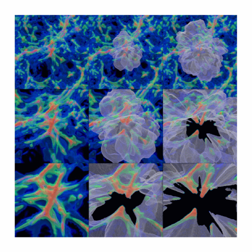
Figure 8.— Volume visualization at $z=20$ of neutral density field (blue – low density, red – high density) and I-front (translucent white surface). Top row panels show a cubic volume $\sim 13.6$ kpc (proper) across, middle row $\sim 6.8$ kpc, and bottom row $\sim 3.4$ kpc. Left column is at the initial time, middle column shows simulation at $t_{*}=3$ Myr for the run with stellar mass $M_{*}=80M_{\odot}$, and the right column shows simulation at $t_{*}=2.2$ Myr for the run with stellar mass $M_{*}=200M_{\odot}$. The empty black region in the lower panels of middle and right columns indicates fully ionized gas around the source, and is fully revealed as the volume visualized shrinks to exclude the I-front that obscures this region in the larger volumes above.

$$F=\int_{r_{t}}^{r_{\rm vir}}\alpha_{B}n_{\rm H}^{2}(r)dr,$$ (21)

where $F$ is the external flux of ionizing photons, $r_{t}$ is the radius at which the I-front is trapped, and $r_{\rm vir}$ is the virial radius of the halo. If we assume that the halo has a singular isothermal sphere density profile $n_{\rm H}(r)\propto r^{-2}$ and an overdensity $\delta_{\rm vir}$, then solving for $r_{t}$ we obtain

$$\frac{r_{t}}{r_{\rm vir}}=\left[1+\frac{9(36\pi)^{1/3}Fm_{\rm H}^{2}\Omega_{m}^{2}}{\alpha_{B}X^{2}M_{\rm vir}^{1/3}\left({\overline{\rho}(z)}\delta_{\rm vir}\right)^{5/3}\Omega_{b}^{2}}\right]^{-1/3},$$ (22)

where ${\overline{\rho}(z)}$ is the mean matter density of the universe at redshift $z$. For $r_{t}^{3}/r^{3}_{\rm vir}\ll 1$, we can neglect the first term in the brackets, to see how this trapping condition depends upon the source and halo parameters and the redshift,

$$\frac{r_{t}}{r_{\rm vir}}\approx\left[\frac{4\pi\alpha_{B}\rho_{0}^{5/3}X^{2}\Omega_{b}^{2}}{9(36\pi)^{1/3}m_{\rm H}^{2}\Omega_{m}^{2}}\right]^{1/3}M_{\rm vir}^{1/9}\delta_{\rm vir}^{5/9}Q_{*}^{-1/2}r^{2/3}(1+z)^{5/3},$$ (23)

where $\rho_{0}$ is the mean matter density at present. The density at the point where the I-front is trapped is

$$n_{t}\equiv n_{\rm H}(r_{t})=\frac{X{\overline{\rho}}(z)\Omega_{b}\delta_{\rm vir}}{3m_{\rm H}\Omega_{m}}\frac{r^{2}_{\rm vir}}{r^{2}_{t}}.$$ (24)

If we use the parameters of the minihalo nearest to our source halo for fiducial values,

$$\frac{r_{t}}{r_{\rm vir}} \approx 0.18\left(\frac{M_{\rm vir}}{2\times 10^{5}M_{\odot}}\right)^{1/9}\left(\frac{r}{220\ {\rm pc}}\right)^{2/3}\left(\frac{\delta_{\rm vir}}{200}\right)^{5/9}$$ (25)

$$\times \left(\frac{Q_{*}}{1.4\times 10^{50}\ {\rm s}^{-1}}\right)^{-1/3}\left(\frac{1+z}{21}\right)^{5/3}$$

and

$$n_{t} \approx 3.6\ {\rm cm}^{-3}\left(\frac{M_{\rm vir}}{2\times 10^{5}M_{\odot}}\right)^{-2/9}\left(\frac{r}{220\ {\rm pc}}\right)^{-4/3}$$

$$\times \left(\frac{\delta_{\rm vir}}{200}\right)^{-1/9}\left(\frac{Q_{*}}{1.4\times 10^{50}\ {\rm s}^{-1}}\right)^{2/3}\left(\frac{1+z}{21}\right)^{-1/3},$$

corresponding to a halo with total mass $M_{\rm vir}=2\times 10^{5}M_{\odot}$ that is exposed to a flux $F=Q_{*}/(4\pi r^{2})$ from a source with luminosity $Q_{*}=1.4\times 10^{50}s^{-1}$ (for a stellar mass $M_{*}=120M_{\odot}$) at a distance $r=220$ pc. Since $M(<R)\propto R$ in a singular isothermal sphere, $M_{\rm HI}/M_{\rm vir}=r_{t}/r_{\rm vir}$, and thus the neutral gas mass for the fiducial case above is $\simeq 5.5\times 10^{3}M_{\odot}$. The density at which the I-front is trapped is much smaller than the central density expected for a truncated isothermal sphere (Shapiro, Iliev, & Raga 1999), $n_{\rm H,0}\simeq 30$ cm^-3 at $z=20$. Thus, nearby halos trap the I-front well before it reaches the central core. The weak dependence of $r_{t}/r_{\rm vir}$ on halo mass and luminosity implies that trapping is a generic occurrence for halos surrounding single primordial stars.

5. Discussion

We have studied the evolution of the H II region created by a massive Pop III star which forms in the current, standard $\Lambda$CDM universe in a minihalo of total mass $M\sim 10^{6}M_{\odot}$ at a redshift of $z=20$. We have performed a three-dimensional ray-tracing calculation which tracks the position of the expanding I-front in every direction around the source in the pre-computed density field which results from a cosmological gas and N-body dynamics simulation based on the GADGET tree-SPH code. During the short lifetime ($\lesssim$ few Myr) of such a star, the hydrodynamical back-reaction of the gas is relatively small as long as the front is a supersonic R-type, Figure 9.— Position of selected SPH particles within 500 pc of the 120 $M_{\odot}$ star. Red particles are ionized and have a density above 1 cm^-3, all the neutral particles are shown in cyan, while only neutral particles with a density above 4 cm^-3 are colored black. The radius of the shock in the Shu solution at the end of the star’s lifetime, $\sim 100$ pc, is shown as the circle in the center. No SPH particles are shown within that radius. and, to first approximation, we are justified in treating the gas in this “static limit.” At early times, however, when the I-front is still deep inside the minihalo which formed the star, the I-front is expected to make a transition from supersonic R-type to subsonic D-type, preceded by a shock, before it eventually accelerates to R-type again and detaches from the shock, racing ahead of it.

To account for the impact of the expansion of the gas which results from this dynamical phase on the propagation of the I-front after it “breaks out,” we have used the similarity solution of Shu et al. (2002) for champagne flow. This solution allows us to determine when the transition from D-type to R-type and “break-out” occurs and, thereafter, to account for the consumption of ionizing photons in the expanding wind left behind in the central part of the minihalo. In this way, we are able to track the progress of the I-front inside the host minihalo and beyond, as it sweeps outward through the surrounding IGM and encounters other minihalos. This has allowed us to investigate the link, for the first time, between the formation of the first stars and the beginning of cosmic reionization on scales close to the stellar source that could not be resolved in previous three-dimensional studies of cosmic reionization. Among the results of this calculation are the following.

Our simulations allow us to quantify the ionizing efficiency of the first-generation of Pop III stars in the $\Lambda$CDM universe as a function of stellar mass. The fraction of their ionizing radiation which escapes from their parent minihalo increases with stellar mass. For stars in the mass range $80\lesssim M_{*}/M_{\odot}\lesssim 500$, we find $0.7\lesssim f_{\rm esc}\lesssim 0.9$. This high escape fraction for high-mass stars is roughly consistent with the high escape fraction found for such high-mass stars by one-dimensional, spherical, hydrodynamical calculations (Whalen et al. Figure 10.— Top: Mean recombination time of H II region at end of star’s life vs. stellar mass. Bottom: Clumping factor of H II regions at end of star’s life vs. stellar mass. Less massive stars ionize a smaller volume, which implies a higher clumping factor because of clustering around the host halo. 2004; Kitayama et al. 2004). For lower-mass stars, the escape fraction drops more rapidly with decreasing mass, as it takes a longer and longer fraction of the stellar lifetime for the I-front to end the D-type phase by reaching the “break-out” point, detaching from the shock and running ahead as a weak, R-type front to exit the halo. For $M_{*}\lesssim 15-20M_{\odot}$, in fact, we find that the escape fraction should be zero and the I-front is D-type for the whole life of the star. More importantly, we find that this threshold mass is very sensitive to the hydrodynamic evolution of the I-front in the D-type phase. Given the great uncertainty regarding the interaction of the stellar radiation and the gas immediately surrounding the star, a definitive answer to this question can only be obtained through three-dimensional gas dynamical simulations with radiative transfer that properly resolve the accretion flow onto the star.

Once the H II region escapes the confines of the parent minihalo, the reionization of the universe begins. Our simulations yield the ratio of the final total mass ionized by each of these first-generation Pop III stars to their stellar mass. We find that, for $M_{*}\gtrsim 80M_{\odot}$, this ratio is about 60,000, roughly half the number of H ionizing photons released per stellar atom during the lifetime of these stars, independent of stellar mass.

We can obtain a very rough estimate of how effective Pop III stars are at reionizing the universe by assuming that all the stars have the same mass and form at the same redshift, each in its own minihalo of mass $\sim 10^{6}M_{\odot}$. In the limit where the H II regions of individual stars are not overlapping, the ionized mass fraction fraction is given in terms of the halo mass function by $f_{\rm HII}=\rho_{\rm HII}/{\overline{\rho_{\rm H}}}$ where $\rho_{\rm HII}\equiv\eta_{\rm HII}M_{*}dn/d\ln M$ is the mean density of ionized gas, assuming each halo hosts a star of mass $M_{*}$, and ionized a mass $\eta_{\rm HII}$ times the star’s own mass, and ${\overline{\rho_{\rm H}}}$ is the mean mass density of hydrogen (For $M_{*}\simeq 80M_{\odot}$, for example, $\eta_{\rm HII}\simeq 50,000$). Using the mass function of Sheth & Tormen (2002), $dn/d\ln M\simeq 130$ Mpc^-3 in comoving units at $z=20$ for this mass range, we obtain $f_{\rm HII}\simeq 0.1[\eta_{\rm HII}/5\times 10^{4}][M_{*}/80M_{\odot}]$. If, instead, we use the ionized volume $V_{\rm HII}$ obtained directly from our calculations to derive the volume filling factor $f_{\rm V,HII}\equiv V_{\rm HII}dn/d\ln M$ for an $80M_{\odot}$ star, the final ionized volume is $7\times 10^{-4}$ comoving Mpc³, corresponding to a filling factor of $f_{\rm V,HII}(M_{*}=80M_{\odot})\simeq 0.1$. The similarity of the volume and mass ionized fraction indicates that the mean density in the ionized region is approximately equal to the mean density of the universe.

The above estimate is only the instantaneous ionized fraction, since the recombination times of each relic H II region are small fractions of the age of the universe at $z=20$. This implies that many new generations of similar stars would have to form to continuously maintain this ionized fraction. A more conservative estimate of the effect of Pop III stars on reionization would also have to take account of the back-reaction of the starlight from earlier generations of stars on the star formation rate in the minihalos that follow (e.g., Mackey, Bromm, & Hernquist 2003; Yoshida et al. 2003; Furlanetto & Loeb 2005). Since Pop III star formation depends upon the efficiency of H₂ formation and cooling inside minihalos, a background of UV starlight between 11.2 eV and 13.6 eV is capable of suppressing this star formation by photodissociation the H₂ following absorption in the Lyman-Werner bands. It is quite possible that the photodissociating background builds up fast enough that minihalos are “sterilized” against further star formation before such a large fraction of the universe can be reionized in this way (Haiman et al. 1997).

Hydrodynamic feedback due to photoionization heating of the host halo will have a dramatic impact on its ultimate fate. Massive Pop III stars are expected to end their lives either by collapsing to black holes or exploding as pair-instability supernovae (e.g., Madau & Rees 2001; Heger et al. 2003). In both cases, it is important to know the properties of the host halo gas. Our model for the hydrodynamic feedback, in which an ionized, nearly-uniform density bubble bounded by an isothermal shock propagates outward at a few times the sound speed allows for an estimate of the density and size of the bubble at the end of the star’s lifetime. For a lifetime of 2.5 Myr, the final size and density of the bubble are $r_{\rm bubble}\simeq 100$ pc and $n_{\rm bubble}\lesssim 1$ cm^-3. If the star ended its life by exploding, rather than collapsing to a black hole, then the SN remnant evolution inside this low-density bubble and beyond will differ from its evolution in the original undisturbed minihalo gas. This should be taken into account in models of the impact of first-generation SN remnant blast-waves on their surroundings (e.g., Bromm, Yoshida, & Hernquist 2003).

This density can be used to estimate the accretion rate onto a possible remnant black hole, $\dot{M}_{B}\simeq 4\pi G^{2}M_{\rm BH}^{2}\rho/c_{s}^{3}$ (e.g., Bondi & Hoyle 1944; Springel, Di Matteo, & Hernquist 2005). Thus, e.g., for a black hole mass of $100M_{\odot}$ and a sound speed of 15 km s^-1, we obtain $\dot{M}_{B}\sim 2\times 10^{-5}M_{\odot}$ Myr^-1. If we make the optimistic assumption that after a recombination time ($\sim 1.2\times 10^{5}$ yr) the gas can form ${\rm H}_{2}$ molecules and cool back to $\sim 300$ K without escaping from the halo, the accretion rate increases by a factor of $10^{3}$, to $\sim 2\times 10^{-2}M_{\odot}$Myr^-1. These accretion rates are small compared to the Eddington accretion rate $\dot{M}_{\rm Edd}=4\pi GM_{\rm BH}m_{p}/(\epsilon\sigma_{T}c)\simeq 2M_{\odot}$ Myr^-1, where the efficiency factor $\epsilon=0.1$ (see also O’Shea et al. 2005). Such low accretion rates imply that remnant black holes from the first generation of stars are unlikely to be strong sources of radiation. Calculations which do not explicitly take into account this reduction in gas density near the remnant (e.g., Kuhlen & Madau 2005) risk substantially overestimating their radiative feedback as miniquasars. These remnant black holes could begin to emit a substantial amount of radiation only after they encounter some other environment containing cold, dense gas. It is not clear when or whether these black holes would ever encounter such an environment. At the very least, therefore, there should be some delay between the formation of the first generation of stars and the X-ray emission from their remnants, if such emission ever occurs.

Determining the fate of recombining gas in the relic H II regions left behind by the first stars is crucial. The contribution of these relic H II regions from the first-generation Pop III stars to the increasing ionized fraction of the universe during cosmic reionization depends upon their recombination time. Because of clustering around the host halo, the clumping factor and recombination time within the relic H II region depends on the mass of the star; higher stellar masses correspond to lower clumping factors and longer recombination times. The recombination time and clumping factor for a $40M_{\odot}$ star are about 10 Myr and 12, respectively, whereas for a $500M_{\odot}$ star they are about 35 Myr and 3 (see Fig. 10).

When ionized gas within the relic H II region cools radiatively and recombines, the nonequilibrium recombination lags the cooling, which enhances the residual ionized fraction at 10⁴ K, promoting the formation of H₂ molecules which can cool the gas to $T\sim 100$ K and enhance gravitational instability (Shapiro & Kang 1987). This corresponds to “positive feedback” if further star formation results (e.g., Ferrara 1998; Riccotti, Gnedin, & Shull 2001).

Recently, O’Shea et al. (2005) have addressed this issue of possible second generation star formation in the relic H II region of the first Pop III stars. They report that the I-front of the first star will fully ionize the neighboring minihalos and that, when the initial star dies, the dense cores of these ionized neighbor minihalos will be stimulated to form H₂ molecules, leading to the second generation of Pop III stars. This assumes the initial star collapses to form a black hole without exploding as a supernova. We find, however, that the neighboring minihalos are not fully ionized before the initial star dies, since the I-front is trapped by these minihalos and converted to D-type outside the core region, and the photoevaporation time for the minihalo exceeds the lifetime of the ionizing star. It remains to be seen, therefore, if the enhanced H₂ formation which O’Shea et al. (2005) found inside the nearest neighbor minihalo in their simulations of the relic H II region will occur in the presence of the I-front trapping and self-shielding which we report. More work will be required to resolve this question.

Whether H₂ molecules form in abundance or not depends on the density of the recombining gas. As we discussed in §4.4, the highest density of gas in the relic H II region which we found to be fully ionized and, hence, capable of recombining to form ${\rm H}_{2}$ molecules, is a few cm^-3. A rough estimate of the ${\rm H}_{2}$ molecule formation time is given by the recombination time of the gas, $t_{\rm rec}\simeq 10^{5}$ yr. Even if ${\rm H}_{2}$ molecules form, however, it is not certain whether this will promote star formation in neighboring halos. As we have shown, the densest gas located in the center of nearby halos is not ionized. The gas that is ionized is not in the center, and is thus likely to recombine while being ejected from the halo as part of a supersonic, photoevaporative outflow (e.g., Shapiro, Iliev, & Raga 2004). Such gas is less likely to be gravitationally unstable. In future work, we will investigate whether this gas is able to cool and form stars or simply gets evaporated into the diffuse IGM.

Appendix A Mass-conserving SPH Interpolation onto a Mesh

Rather than interpolate directly from the SPH particles to our spherical grid of rays, we first interpolate the density to a uniform rectilinear mesh. The assignment of density to the mesh should conserve mass, which we accomplish as follows. We use a Gaussian kernel

$$W(r,h)=\frac{1}{\pi^{3/2}h^{3}}e^{-r^{2}/h^{2}},$$ (A1)

where $h$ is the smoothing length and $r$ is distance. This kernel is very similar to the commonly-used spline kernel,

$$W(r,h)=\frac{8}{\pi h^{3}}\left\{\begin{array}[]{ll}1-6\left(\frac{r}{h}\right)^{2}+6\left(\frac{r}{h}\right)^{3},&0\leq\frac{r}{h}\leq\frac{1}{2},\\ 2\left(1-\frac{r}{h}\right)^{3},&\frac{1}{2}\leq\frac{r}{h}\leq 1,\\ 0&\frac{r}{h}>1.\end{array}\right.$$ (A2)

In our case, where a spline kernel has been used in the SPH calculation, we find that a Gaussian kernel is sufficient for interpolation purposes, provided we transform the smoothing lengths according to $h_{\rm Gauss}=\pi^{-1/6}h_{\rm spline}/2$.

For interpolation to a uniform rectilinear mesh with cell size $\Delta_{c}$, we wish to find the mean density within a cell centered at $(x,y,z)$ contributed by a particle with smoothing length $h$ located at the origin,

$${\overline{W}}({\bf r},h)\equiv\frac{1}{\Delta_{c}^{3}}\int_{V}W(r,h),$$ (A3)

where the integral is over the volume of the cell. Since the kernel is a Gaussian, the spatial integral separates into three separate ones, so that

$${\overline{W}}({\bf r},h)=\frac{1}{8\Delta_{c}^{3}}\Xi(x)\Xi(y)\Xi(z),$$ (A4)

where

$$\Xi(s)\equiv{\rm erf}\left[\frac{s+\Delta_{c}/2}{h}\right]-{\rm erf}\left[\frac{s-\Delta_{c}/2}{h}\right].$$ (A5)

The value of the density averaged over a cell centered at ${\bf r}_{c}$ is thus

$${\overline{\rho}}({\bf r}_{c})=\sum_{i}m_{i}{\overline{W}}({\bf r}_{c}-{\bf r}_{i},h_{i}),$$ (A6)

where the sum is over all particles $i$ such that ${\overline{W}}({\bf r}_{c}-{\bf r}_{i},h_{i})/{\overline{W}}(0,h_{i})>\epsilon$, so as not to needlessly sum over particles with a negligible contribution. We find that a value $\epsilon=10^{-5}$ is sufficient for our purposes.

References

- (1) Abel, T., Bryan, G. L., & Norman, M. L. 2002, Science, 295, 93
- (2) Barkana, R., & Loeb, A. 2001, Phys. Rep., 349, 125
- (3) Bond, J. R., Arnett, W. D., & Carr, B J. 1984, ApJ, 280, 825
- (4) Bondi, H., & Hoyle, F. 1944, MNRAS, 104, 273
- (5) Bromm, V., Coppi, P. S., & Larson, R. B. 1999, ApJ, 527, L5
- (6) Bromm, V., Coppi, P. S., & Larson, R. B. 2002, ApJ, 564, 23
- (7) Bromm, V., Kudritzki, R. P., & Loeb, A. 2001, ApJ, 552, 464
- (8) Bromm, V., & Larson, R. B. 2004, ARA&A, 42, 79
- (9) Bromm, V., & Loeb, A. 2003, Nature, 425, 812
- (10) Bromm, V., & Loeb, A. 2004, NewA, 9, 353
- (11) Bromm, V., Yoshida, N., & Hernquist, L. 2003, ApJ, 596, L135
- (12) Cen, R. 2003, ApJ, 591, 12
- (13) Ciardi, B., & Ferrara, A. 2005, Space Sci. Rev., 116, 625
- (14) Ciardi, B., Ferrara, A., & White, S.D.M. 2003, MNRAS, 344, L7
- (15) Couchman, H. M. P., & Rees, M. J. 1986, MNRAS, 221, 53
- (16) Ferrara, A. 1998, ApJ, 499, L17
- (17) Franco, J., Tenorio-Tagle, G., & Bondenheimer, P. 1990, ApJ, 349, 126
- (18) Furlanetto, S. R., & Loeb, A. 2005, ApJ, in press (astro-ph/0409656)
- (19) Gnedin, N. Y., & Ostriker, J. P. 1997, ApJ, 486, 581
- (20) Górski, K. M., Hivon E., Banday A. J., Wandelt, B. D., Hansen, F. K., Reinecke, M., & Bartelmann, M. 2005 ApJ, 622, 759
- (21) Haiman, Z., Abel, T., & Rees, M. J. 2000, ApJ, 534, 11
- (22) Haiman, Z. & Holder, G. P. 2003, ApJ, 595, 1
- (23) Haiman, Z., Rees, M. J., & Loeb, A. 1997, ApJ, 476, 458
- (24) Haiman, Z., Thoul, A. A., & Loeb, A. 1996, ApJ, 464, 523
- (25) Heger, A., Fryer, C. L., Woosley, S. E., Langer, N., & Hartmann D. H. 2003, ApJ, 591, 288
- (26) Iliev, I. T., Shapiro, P. R., & Raga, A. C. 2005, MNRAS, 361, 405
- (27) Kitayama, T., Yoshida, N., Susa, H., & Umemura, M. 2004, ApJ, 613, 631
- (28) Kogut, A., et al. 2003, ApJS, 148, 161
- (29) Kuhlen, M., & Madau, P. 2005, MNRAS, in press (astro-ph/0506712)
- (30) Mackey, J., Bromm, V., & Hernquist, L. 2003, ApJ, 586, 1
- (31) Madau, P., & Rees, M. J. 2001, ApJ, 551, L27
- (32) Nakamura, F., & Umemura, M. 2001, ApJ, 548, 19
- (33) O’Shea, B. W., Abel, T., Whalen, D., & Norman, M. L. 2005, ApJ, 626, L5
- (34) Oh, P., & Haiman, Z. 2003, MNRAS, 346, 456
- (35) Omukai, K., & Inutsuka, S. 2002, MNRAS, 332, 59
- (36) Omukai, K., & Palla, F. 2001, ApJ, 561, L55
- (37) Omukai, K., & Palla, F. 2003, ApJ, 589, 677
- (38) Ricotti, M., Gnedin, N. Y., & Shull, M. J. 2001, ApJ, 560, 580
- (39) Schaerer, D. 2002, A&A, 382, 28
- (40) Shapiro, P. R., & Giroux, M. L. 1987, ApJ, 321, L107
- (41) Shapiro, P. R., Iliev, I. T., Alvarez, M. A., & Scannapieco, E. 2005, ApJ, submitted (astro-ph/0507677)
- (42) Shapiro, P. R., Iliev, I. T., & Raga, A. C. 1999, MNRAS, 307, 203
- (43) Shapiro, P. R., Iliev, I. T., & Raga, A. C. 2004, MNRAS, 348, 753
- (44) Shapiro, P. R., & Kang, H. 1987, ApJ, 318, 32
- (45) Sheth, R. K., & Tormen, G. 2002, MNRAS, 329, 61
- (46) Shu, F. H., Lizano S., Galli, D., Cantó, J., & Laughlin, G. 2002, ApJ, 580, 969
- (47) Sokasian, A., Yoshida, N., Abel, T., Hernquist, L., & Springel, V. 2004, MNRAS, 350, 47
- (48) Spergel, D. N., et al. 2003, ApJS, 148, 175
- (49) Spitzer, L. 1978, Physical Processes in the Interstellar Medium (New York: Wiley)
- (50) Springel, V., Di Matteo, T., & Hernquist, L. 2005, MNRAS, in press (astro-ph/0411108)
- (51) Springel, V., Yoshida, N., & White, S. D. M. 2001, NewA, 6, 79
- (52) Tan, J. C., & McKee, C. F. 2004, ApJ, 603, 383
- (53) Tegmark, M., Silk, J., Rees, M. J., Blanchard, A., Abel, T., & Palla, F. 1997, ApJ, 474, 1
- (54) Venkatesan, A., Tumlinson, J., & Shull, J. M. 2003, ApJ, 584, 621
- (55) Whalen, D., Abel, T., & Norman, M. 2004, ApJ, 610, 14
- (56) Wyithe, J. S. B., & Loeb, A. 2003, ApJ, 588, L69
- (57) Yoshida, N., Abel, T., Hernquist, L., & Sugiyama, N. 2003a, ApJ, 592, 645
- (58) Yoshida, N., Bromm, V., Hernquist, L. 2004, ApJ, 605, 579
- (59) Yu, Q., 2005, ApJ, 623, 683