The VIRMOS deep imaging survey IV:
Near-infrared observations

In this paper we present a new deep, wide-field near-infrared imaging survey. Our $J-$ and $K-$band observations in four separate fields (0226-04, 2217+00, 1003+02, 1400+05) complement optical $BVRI$, ultraviolet and spectroscopic observations undertaken as part of the VIMOS-VLT deep survey (VVDS). In total, our survey spans $\sim 400\leavevmode\nobreak\ \rm{arcmin}^{2}$. Our catalogues are reliable in all fields to at least $K\sim 20.75$ and $J\sim 21.50$ (defined as the magnitude where object contamination is less than 10% and completeness greater than 90%).

Taken together these four fields represents a unique combination of depth, wavelength coverage and area. Most importantly, our survey regions span a broad range of right ascension and declination which allow us to make a robust estimate of the effects of cosmic variance. We describe the complete data reduction process from raw observations to the construction of source lists and outline a comprehensive series of tests carried out to characterise the reliability of the final catalogues. From simulations we determine the completeness function of each final stacked image, and estimate the fraction of spurious sources in each magnitude bin. We compare the statistical properties of our catalogues with literature compilations. We find that our $J-$ and $K-$selected galaxy counts are in good agreement with previously published works, as are our $(J-K)$ versus $K$ colour-magnitude diagrams. Stellar number counts extracted from our fields are consistent with a synthetic model of our galaxy. Using the location of the stellar locus in colour-magnitude space and the measured field-to-field variation in galaxy number counts we demonstrate that the absolute accuracy of our photometric calibration is at the $5\%$ level or better. Finally, an investigation of the angular clustering of $K-$ selected extended sources in our survey displays the expected scaling behaviour with limiting magnitude, with amplitudes in each magnitude bin in broad agreement with literature values.

In summary, these catalogues will be an excellent tool to investigate the properties of near-infrared selected galaxies, and such investigations will be the subject of several articles currently in preparation.

1 Introduction

Galaxy surveys selected in near-infrared wavelengths ($1.1-1.5\mu$) provide some well-established advantages with respect their optically-selected counterparts. A census conducted at these longer wavelengths can provide flux measurements in an object’s rest-frame optical bandpass at intermediate redshifts, which can in turn be easier to relate to physically interesting quantities such a galaxy’s total mass in stars. Any credible model of galaxy formation must predict how this stellar mass function evolves with redshift. In addition, the predicted number densities and spatial distribution of objects lying at the reddest outer reaches of the optical-infrared colour-magnitude diagram ( “the extremely red objects” or EROs) also depend very sensitively on one’s assumed model of galaxy formation. Understanding this red outlier population and how it relates to UV-selected star-forming galaxies at higher redshifts and massive ellipticals at the present day has become one of the most important questions in observational cosmology. Near-infrared data is also crucial to compute accurate photometric redshifts in the $1<z<2$ redshift range, where measuring spectroscopic redshifts with a red-optimised spectrograph can be challenging. Until recently, however, the small format of near-infrared detectors (and the much higher ground–based brightness of the sky at longer wavelengths) has made surveys of the near-infrared selected Universe a very time-consuming undertaking. Only in the last few years, with the advent of larger-format detectors, has it become practical to survey deeply larger areas of the sky in the near IR to cosmologically significant redshifts.

In this paper we describe a new deep near-infrared survey. The observations presented here cover a total area of $\sim 400$ arcmin² over four separate fields in both $J$ and $K$ bands. Each of the four fields reaches a completeness limit (defined as the magnitude at which $90\%$ of simulated point sources are recovered from the images) of at least $22.0$ magnitudes in $J$ and 20.75 in $K$. This represents an intermediate regime between, for example, very deep surveys like FIRES (Labbé et al., 2003) which covers a few square arcminutes to depth of $K\sim 24$, and shallower surveys (Daddi et al., 2000; Drory et al., 2001) which reach to around $K\sim 19$ over several hundred square arcminutes. The current survey has been undertaken in the context of the VIMOS-VLT deep survey (Le Fèvre et al., 2005), and the near-infrared data presented here complements optical and ultraviolet imagery (McCracken et al., 2003; Radovich et al., 2004), as well as 2.4Ghz VLA radio data (Bondi et al., 2003). To $K<20.5$, 766 objects from our catalogue have been observed spectroscopically in the first epoch VVDS (Le Fèvre et al., 2005).

Our primary objective in this paper is to describe in detail how our near-infrared catalogues were prepared and to quantify their reliability and completeness. Future papers will present more detailed analysis of our $J-$ and $K-$selected samples and in particular the clustering properties of objects with extreme colours. All magnitudes quoted in this paper are in the Vega system unless otherwise stated.

2 Observations

The survey described in this article covers in $J$ and $K$ bands four different regions of the sky spanning a wide range of right ascension so that at least one field is observable throughout the year. Each of these regions has corresponding deep optical imaging, taken with either the Canada France Hawaii Telescope’s (CFHT) CFH12K camera (McCracken et al., 2003; Le Fèvre et al., 2004) or the ESO 2.2 metre telescope’s Wide-Field Imager (Radovich et al., 2004). The observations described this paper were carried out at the ESO New Techonology Telescope using the SOFI Near Infrared imaging camera (Moorwood et al., 1998) with the $J$ and the $K_{s}$ filters. The $K_{s}$ filter is bluer and narrower than the standard near-infrared $K-$band filter, and so is less affected by the thermal background of the atmosphere and of the telescope (Wainscoat & Cowie, 1992). Throughout this paper our $K$ magnitudes are in fact “$K_{s}$” magnitudes. SOFI is equipped with a Rockwell Hawaii HgCdTe 1024x1024 array and observations were made with the Large Field (LF) objective, corresponding to a field-of-view of $4.9\times 4.9$ ″and a pixels scale of $0.288$ ″/pixel.

The observations took place over a series of runs from September 1998 to November 2002. Each targetted field was observed in a series of pointings in a raster configuration, each separated from surrounding ones by $4^{\prime}15$″in both right ascension and in declination, in order to ensure a non negligible overlap between adjacent pointings. Figure 1 shows the layout of our $K-$band observations of field $0226-04$ as an example.

Figure 1: Layout of the observed $K-$band pointings for field $0226-04$. The raster configuration chosen in order to secure a non-negligible overlap between adjacent pointings is clearly visible. Each pointing is is turn observed through a series of jittered exposures, with jitter box size of 30 ″(see text for more details).

The well known peculiarities of infrared observations (higher and more variable sky background, strong and variable absorption bands) dictated our observational strategy. Total integration time per pointing was around 1 hour for the $J$-band and three hours for $K-$band exposures, with some pointings being observed for up to four hours in $K-$band. Each integration consisted of many shorter jittered exposures with the telescope being offset by random amounts within a box of size 30″. The jittered observations were usually grouped in observation sequences each typically one hour long. Each individual short exposure in both bands was 1.5 minutes long, with DIT = 15 (meaning a detector integration time of 15 seconds was used) and NDIT = 6 in $J$ (indicating that six of these 15 second integrations were used) and with DIT = 10 sec and NDIT = 9 in $K$. For the observations of the standard stars we adopted DIT = 2 ( DIT = 1.2) sec in $J$ (in $K$) and NDIT = 15 to avoid saturation.

The four observed areas are listed in Table 1 together with the centres for each of the pointings (J2000), observing runs when the observations were performed, total exposure times and galactic extinction in $J-/K-$ band computed using the COBE/DIRBE dust maps (Schlegel et al., 1998). Unfortunately, poor weather conditions partially hampered our efficiency and reduced our final total areal coverage.

List of observed pointings
field	pointing	RA	Dec		$J-$band			$K-$band
		(2000)	(2000)	Obs run	$t_{exp}$	$A_{J}$	Obs run	$t_{exp}$	$A_{K}$
$0226-04$	n1	02 27 14	-04 14 18	nov02	60	0.023	sep98	195	0.010
	n2	02 26 57	-04 14 18	sep00	55	0.024	sep98	214.5	0.010
	n3	02 26 40	-04 14 18	nov02	60	0.024	sep98 & nov98	217.5	0.010
	n4	02 27 14	-04 18 33	nov02	66	0.023	nov98	192	0.009
	n5	02 26 57	-04 18 33	nov02	88	0.023	nov98	180	0.009
	n6	02 26 40	-04 18 33	sep00	60	0.024	nov98	196.5	0.010
	n7	02 27 14	-04 22 48	sep00	60	0.022	nov98	180	0.009
	n8	02 26 57	-04 22 48	nov02	60	0.023	nov99	180	0.009
	n9	02 26 40	-04 22 48	nov02	60	0.025	nov99	180	0.010
$2217+00$	n1	22 18 08	00 19 45	sep00	60	0.059	sep98	255	0.024
	n2	22 17 51	00 19 45	sep00	60	0.058	sep98	270	0.024
	n3	22 17 34	00 19 45	nov02	60	0.055	sep00 & nov02	240	0.022
	n4	22 18 08	00 15 30	sep00	60	0.063	nov98 & nov02	210	0.026
	n5	22 17 51	00 15 30	sep00	60	0.064	–	–	–
$1003+01$	n1	10 03 56	01 58 54	apr99	45	0.022	mar99	180	0.010
	n2	10 03 39	01 58 54	apr99	45	0.019	mar99	180	0.010
	n3	10 03 22	01 58 54	apr00	60	0.018	nov99	180	0.010
	n4	10 03 56	01 54 39	apr99 & nov02	60	0.023	mar99 & apr99	181.5	0.009
	n5	10 03 39	01 54 39	apr99 & nov02	60	0.020	nov98 & mar99	195	0.009
	n6	10 03 22	01 54 39	–	–	–	apr00	180	0.010
$1400+05$	n1	14 00 18	05 13 30	apr00	60	0.022	mar99	181.5	0.010
	n2	14 00 01	05 13 30	–	–	–	mar99 & apr00	222	0.010

Table 1: List of fields observed. See text for more details.

3 Data reduction

3.1 Science frames

Data reduction of the scientific frames in both filters included the usual standard steps: dark subtraction, flat fielding and sky subtraction. We now outline the basic processing steps followed. The darks to be subtracted were computed using the IRAF task darkcombine from a series of darks obtained with the same DIT and NDIT as the science frames. The well known complex bias behaviour of the Rockwell Hawaii array means that there is a dependence of the detector dark on time and illumination history, and this manifests itself as a pattern which remains in all the images after dark subtraction. This is visible as a discontinuity between the lower upper part of the array and the upper lower part of the array (i.e. were the two upper quadrants join the two lower quadrants). This pattern is a purely additive component and it is removed in the sky subtraction step as it changes little in images in the same stack of observations.

Flat-field frames were obtained for both bands with the ON-OFF procedure as described in the SOFI manual. We carefully checked whether our flat-field frames contained the large jump between the lower and upper part of the array which is a signature of a remaining dark residual, rejecting those frames which had a non-negligible dark residual. Using IRAF’s flatcombine task we were able to derived from the remaining flats the final $J$ or $K$ flat. To test the accuracy of the ON-OFF flat field correction, we compared the counts observed for each photometric standard star in different array positions. The rms on the mean was always of the order of a few percent for both bands (and usually below $4\%$).

Before proceeding with the data reduction, we checked the quality of the images and rejected those with full-width half-maximum (FWHM) values larger than $1.\arcsec 3$ or those which were badly affected by sky–transparency fluctuations based on the flux measurements of a chosen reference star. The exposure times quoted in Table 1 are those obtained after this step.

We next used IRAF DIMSUM package to subtract the sky from the dark subtracted, flat fielded, science images (Stanford et al., 1995). DIMSUM was used in a two step process and on sets of 20-30 images belonging to the same observation sequence.

As a first step for each image 6 neighbouring images (3 minimum for the images at the end/beginning) from the same observation sequence were selected to obtain an initial sky estimate. The sky subtracted images were then used to identify the image regions covered by the objects. In this way for each image an object mask was defined and was used to exclude those regions from a second, final pass of sky estimation and subsequent subtraction.

Finally, the second pass sky subtracted images of the same observation sequence were combined in a stacked image by using the task dithercubemean from the IRDR software (Sabbey et al., 2001). This task uses bi-linear interpolation to register the input frames, taking into account pixel weights, based on image variance, exposure time and pixel gain (which is calculated using superflat field image calculated from all the sky subtracted images; see Sabbey et al. (2001) for more details).

A final weight map was also produced by combining individual image weights. At the end of these data reduction steps usually one or two (three or four for $K-$band observations) coadded images and their relative weight maps were produced for each pointing in $J-$band, depending on how the observations were sequenced.

Figure 2 shows the FWHM seeing distribution for the different coadded $K-$band images for each of the four fields. Tables 2 and 3 list for each field and each band the median FWHM seeing as measured in the final mosaicked image (for the $K-$band images this value is shown by the dashed lines in Figure 2).

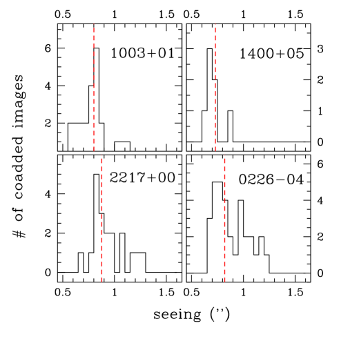
Figure 2: FWHM seeing distribution of the coadded images for each field observed in $K-$band. The dashed line shows the median seeing measured in the final mosaicked image. Note that in all cases this value is below $1\arcsec$. All images with seeing higher than $1.\arcsec 3$ were discarded, and are not shown in this plot.

3.2 Astrometric calibration

Astrometric calibration on the coadded images was performed in two steps for all our images. We first computed a linear astrometric solution using the astrometric catalogue of the United States Naval Observatory (USNO)-A2.0 (Monet, 1998), which provides the positions of $0.5\times 10^{8}$ sources. The area covered by each coadded image usually contained around 10 objects (after removal of saturated and extended sources). This first astrometric solution was then improved by using a catalogue of sources extracted from the resampled $I-$band images which is used as a reference catalogue for all the other optical bands (see (McCracken et al., 2003), and the similar procedure adopted for the $U-$band in Radovich et al. (2004)). As the surface density of these objects is much higher than that of USNO-A2.0, a much higher accuracy in the relative astrometric solution can be obtained. Such accuracy allows us to match sources at the sub-pixel level between optical and infra-red bands.

The quality of the astrometry in the final $K-$band mosaicked images is shown in figure 3 for the four fields. Radial residuals between $K-$band and $I-$band positions for unsaturated, point-like sources are plotted for each of the four mosaicked fields. The inner circle and the outer circle show in each field enclose 68% and 90% of all objects, indicating that we have reached the level of sub-pixel accuracy in the relative astrometry between $I-$band and $K-$band images (the achieved RMS positional accuracy, defined as the radius enclosing 68% of the objects, is for all four fields around $\sim 0.\arcsec 2$). Similar values of radial residuals are obtained between $J-$band and $I-$band positions. The RMS accuracy of our absolute astrometric solution is therefore of the same order of that obtained for $I-$band data, that is $\sim 0.\arcsec 3$ (see McCracken et al. (2003)).

Figure 3: Radial residuals between $K-$band and $I-$band positions for unsaturated, point-like sources for each of the four fields. The inner and outer circles enclose 68% and 90% of all objects respectively. The dashed lines cross each other at the position of the centroid of the residuals distribution.

3.3 Photometric calibration

The photometric calibration was performed using standard stars from the list of near-infrared NICMOS standard stars (Persson et al., 1998). At least two standard stars were observed each night at low airmass ($sec(z)<1.3$), at intervals of roughly two hours, in both $J$ and $K$ bands. Each standard star was observed in 5 different array positions: once near the center of the array and once in each of the four quadrants. These images were dark subtracted and flat fielded according to the procedure discussed above. Sky subtraction was obtained by subtracting the median of the four adjacent images (usually the standard star fields are empty of bright stars).

Instrumental aperture magnitudes for the standard stars were computed within an $8\arcsec$ radius and were airmass corrected assuming an atmospheric extinction coefficient of 0.1 (0.05) in magnitudes/airmass in $J$ ($K$) bands (based on recent measurements in LaSilla, see SOFI home page at ESO: www.ls.eso.org/lasilla/sciops/ntt/sofi/index.html). We estimated the actual zero point for each night by comparing the instrumental magnitudes with those quoted in the literature. This way we obtained for each coadded image an absolute photometric calibration.

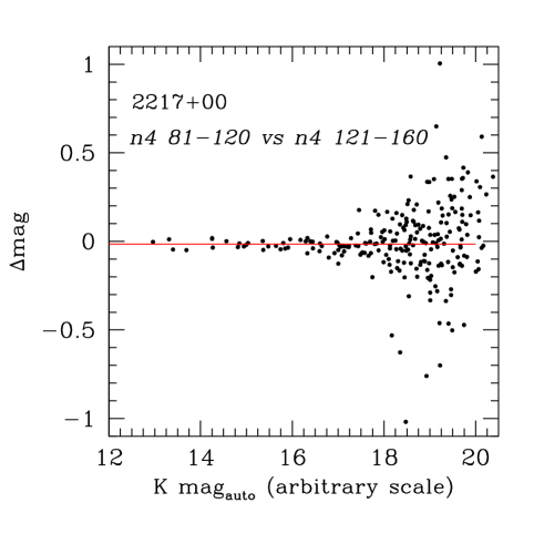
Figure 4: Comparison between the magnitude of corresponding objects in two different $K-$band coadded images of the same pointing. The sequence of images $n4\leavevmode\nobreak\ 81-120$ was observed during the run of November 1998, while $n4\leavevmode\nobreak\ 121-160$ was observed during the run of November 2002. The agreement for the photometry of these two coadded images is quite good (the mean value of the magnitude difference is only $\Delta mags=-0.015$).

Not all our nights were of excellent photometric quality, and therefore a refinement of this first photometric solution was needed. After correcting each coadded image to one second exposure time, to zero airmass and scaling to an arbitrary zero point (normally we chose 30) we improved on this first solution in two steps.

For different coadded images of the same pointing, when available, we compared the magnitude of the point–like brighter objects in common using SExtractor’s (Bertin & Arnouts, 1996) MAG_AUTO measurements to perform the comparison. In this way were able to check for possible photometric offsets between different coadded images of the same pointing. In case of discrepancies we anchored the zero point to the coadded image with the best photometric quality (based on the quality both of its night of observation and of the specific sequence used to build it). Figure 4 shows as an example the comparison between two different coadded $K-$band images of pointing n4 of field $2217+00$, the first taken during the run of November 1998 and the second during the run of November 2002. In this case the agreement between these two coadded images is quite good. In other cases a shift had to be introduced in order to put the different coadded images of the same pointing on the same zero point scale. The size of these shifts was in a few extreme cases as large as 0.3 mags, but mostly below 0.1 mags.

As a second step, we used the stars in common in the overlapping areas between different pointings to define a common photometric scale for each field, assuring the homogeneity of the survey photometry. In this case the few brightest non saturated stars in common enabled us to define a common photometric solution for the different pointing through scaling factors, to be used when building the final mosaicked image of the field. The corresponding shifts introduced in the zero point of the fields to be corrected were always below 0.1 mags.

We took advantage of the repeated observations of the same pointing to estimate the random photometric errors in the final mosaicked images. Following the same procedure outlined in detail in the following Sections, we produced for field $1400+05$ 3 mosaicked $K-$band images, each corresponding to one hour of exposure time, and extracted a photometric catalogue from each of these images. By comparing the magnitudes measured for the same object in the three independent one hour stacks, we obtained a direct estimate of the random photometric errors present in our $K-$band data, including flat-fielding and/or background subtraction inaccuracies (all the direct error estimate have been divided by $\sqrt{3}$ to take into account the shorter exposure time for the individual stacks). Figure 5 shows the comparison of such direct error estimate with the errors obtained by SExtractor and with the errors computed from the simulations used in Sect. 4.1 to estimate completeness of our fields. The errors obtained by SExtractor are always lower, usually by a factor of 2, than the more realistic direct error estimate. The errors obtained from simulations are slightly lower than the direct error estimate: they refer to stellar objects, and are therefore less affected by errors in background determination, especially at bright magnitudes. A similar trend is observed for $J-$band magnitudes errors: the estimate provided by SExtractor is lower by a factor of roughly two than the directly measured errors. A realistic estimate of random photometric errors as a function of object magnitude has to be taken into account when e.g. using these data for photometric redshift determination (see Bolzonella et al. 2005, in preparation).

Figure 5: Root-mean-square magnitude errors as a function of $K-$band magnitude. See text for more details.

3.4 Preparation of final stacks

Once the astrometric and photometric solutions were computed for all the coadded images of each field, these images, together with their weight maps, were combined to produce the final stacks and their weight maps. This is carried out in a two-step process by using Swarp, an image resampling tool (Bertin et al., 2002). This process does not differ from that described in detail for the stacking of optical images described in McCracken et al. (2003), and therefore the interested reader should check there for its details. The final mosaicked images has the same pixel scale (0”.205/pixel) and orientation as the final optical images (McCracken et al., 2003). For each field and band these images were corrected for the mean galactic extinction at the centre of the field as derived from the maps of Schlegel et al. (1998).

3.5 Catalogue preparation

We used SExtractor (Bertin & Arnouts, 1996) to extract sources from the stacked images and their weight maps. For objects to be included in our $J-$ or $K-$band catalogues they must contain at least 3 contiguous pixels above the detection threshold of $1.1\sigma$, giving a minimum signal to noise ratio per source of $1.9\sigma$ for this per-pixel threshold. This conservative threshold means we minimise the number of spurious detections while not adversely affecting our completeness (see later). For the mosaicked image of field $0226-04$ a chi-squared $BVRIK$ image was constructed (Szalay et al., 1999), and for the $J-$ and $K-$band catalogues, image detection was performed using such an image in SExtractor double–image detection mode, with similar extraction parameters as those quoted above (the interested reader should refer to (McCracken et al., 2003) for more details on the chi-squared image construction). In our catalogues magnitudes were measured using the SExtractor parameter MAG_AUTO. This parameter is intended to give a precise estimate of total magnitudes for extended objects, and is inspired by Kron’s first moment algorithm (Kron, 1980). We adopted a minimum Kron radius $R_{min}=1^{\prime\prime}.5$, that is when objects are faint and unresolved MAG_AUTO magnitudes revert to simple aperture magnitudes. Using the same simulations adopted to test the completeness of our catalogues (see Sect. 4.1 ) we verified that MAG_AUTO was a reliable estimate of the input total magnitude of the simulated objects and that the systematic loss of flux was always smaller, in the range of magnitudes of interest, than the dispersion in the magnitudes recovered. The catalogues were visually inspected and noisy border regions of the mosaicked images were masked out together with circular areas surrounding bright objects.

The total area of our survey, after bad regions are excised, is $389$ arcmin² in $J-$band and $430$ arcmin² in $K-$band. The total number of detected sources is 6433 down to $J=22.00$ (7823 down to $J=22.25$) and 8105 down to $K=20.75$ (9539 down to $K=21.00$). Tables 2 and 3 show for each field the final area covered and the number of objects detected down to different magnitude limits.

3.6 Star-galaxy separation

The separation of extended from point-like sources was performed separately for each field and each band using the SExtractor flux_radius parameter. This parameter, denoted as $r_{1/2}$, measures the radius that encloses 50% of the object’s total flux. For point-like sources $r_{1/2}$ is independent of magnitude and depends only of the image seeing. As the seeing is quite uniform across our mosaicked images for each field, a plot of $r_{1/2}$ vs. $J-$, or $K-$band magnitude clearly defines the stellar locus. Heavy dots in figure 6 show, for each field in $K-$band, the point-like objects selected using this classifier. The histogram on the right hand side of each panel illustrates for each field the distribution of $r_{1/2}$ for magnitudes brighter than those deemed feasible for a reliable star-galaxy separation. The stellar locus is clearly visible in this plot. A similar plot was also used to select stars in the $J-$band images.

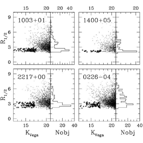
Figure 6: Half-light radius ($r_{1/2}$) as a function of $K-$band magnitudes for each of our four fields. Heavy dots show point like sources. The histogram on the right hand side shows clearly the locus of point-like sources for objects brighter than the classification limit. Fainter than this magnitude ($K\sim 17$) the star-galaxy separation becomes unreliable.

4 Data quality assessment

In these subsections we present a series of quality assessment tests carried out on the catalogues prepared in the previous sections.

4.1 Completeness and contamination

A simple estimate of our limiting magnitude can be obtained by using the background RMS $\sigma$ provided by SExtractor to compute, for each stacked image, the corresponding $3\sigma-$ ($5\sigma-$) magnitude limits. The formula is $mag(n\sigma)=z_{p}-2.5log(n\sigma\sqrt{A})$, were n=3(5), $z_{p}$ is the zero point and $A$ is the area of an aperture whose radius is the average FWHM of point like sources (see Tables 2 and 3). The values estimated this way do not vary much from field to field, and are $mag(3\sigma)\sim 23.4$ and $mag(5\sigma)\sim 22.9$ for the $J-$band images, while are $mag(3\sigma)\sim 22.6$ and $mag(5\sigma)\sim 22.1$ for the $K-$band images. These values can be regarded as indicative lower limits on the detectability of objects in our catalogues.

To better characterise the photometric properties of our images we carried out an extensive set of simulations. For each mosaicked image and for each filter a list of random positions was generated and cross-checked with the position of the real sources to reject cases of possible overlapping between generated random positions and bright real sources positions. The remaining list of coordinates was used to add to the stacks artificial stars distributed uniformly in the range $17.5<J/K<25$. SExtractor was then run on these images with the same parameters adopted for the detection of real objects and the resulting catalogues were cross-correlated with the input list of artificial stars. The process was repeated until a robust statistic was obtained (more than 5000 objects per half-magnitude bin) and the ratio $n_{\rm{input}}/n_{\rm{output}}$ was estimated in bins on 0.5 mags. The results are plotted in Figures 7 and 8 for each field, and the values $mag_{\rm{comp}}$ and $mag_{\rm{lim}}$, corresponding respectively to $90\%$ and $50\%$ completeness level, are shown in Tables 2 and 3. Such completeness limits and curves assume that the profile of the source is point–like and therefore should be considered only as upper limits. The true limiting magnitude of an extended source will depend on its light–profile and actual size and can be up to one magnitude brighter for low surface brightness objects, see eg. Cristóbal-Hornillos et al. (2003). For field $0226-04$, where the extraction was done on the BVRIK chi-squared image, the values quoted for completeness, being obtained from the $J$ and $K-$band mosaicked images only, are a conservative estimate, irrespective of color, for the detectability of objects in the chi-squared image. For each field we also measured incompleteness as a function of position across the mosaicked image. Such tests did not show any significant variation at $m=mag_{\rm{comp}}$ across the mosaicked images (except for the small areas around bright stars, those masked out in the final catalogue).

Figure 7: Ratio of detected input sources as a function of input magnitude for $J-$band. The input catalogue consists of a flat distribution of simulated point-like sources. The dotted lines show the adopted 50% and 90% completeness magnitudes for each field.

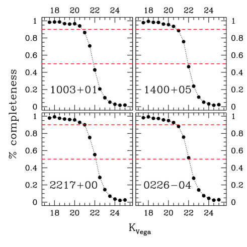
Figure 8: Ratio of detected input sources as a function of input magnitude for $K-$band. The input catalogue consists of a flat distribution of simulated point-like sources. The dotted lines show the adopted 50% and 90% completeness magnitudes for each field.

To complete the characterisation of the photometric properties of our fields we estimated contamination rates as a function of magnitude bins. Each mosaicked image was multiplied by $-1$ and detection of (obviously spurious) objects was performed on this inverse image using the same parameters adopted for detecting objects on the mosaicked image. For the field F02, where the detection was carried out using the chi-squared image, we used the same technique described in McCracken et al. (2003), that is the detection of fake objects was performed on the inverse image using the chi-squared BVRIK image as the reference image. Tables 2 and 3 list, for each field and band, $m_{\rm{cont}<10\%}$: the center of the faintest 0.5 mags bin where contamination by spurious sources is below 10%. For the magnitude limit for the scientific analysis of each of our fields we adopted the conservative choice of the brightest between $m_{\rm{comp}}$ and $m_{\rm{cont}<10\%}$. As expected, field $0226-04$ has the lowest contamination rate at the completeness limits of the survey, confirming the effectiveness of the chi-squared detection image technique in reducing the number of spurious detections.

field name	seeing	$m_{comp}$	$m_{lim}$	$m_{cont<10\%}$	Area	$N_{TOT}$	N($m<22.00$)	N($m<22.25$)
	arcsec				arcmin2
$0226-04$	1.05	22.25	23.25	23.00	162.6	12327	2604	3144
$2217+00$	1.00	21.90	22.90	21.75	102.5	6676	1659	1949
$1003+01$	0.90	22.25	22.90	21.50	102.7	8072	1689	2125
$1400+05$	1.20	22.00	23.15	21.90	23.4	1589	336	408

Table 2: For each field for $J-$band data this table lists $mag_{comp}$, i.e. the center of the 0.5 mag bin where 90% of point–like sources are retrieved, $mag_{\rm{lim}}$ i.e. the center of the 0.5 mag bin where 50% of sources are retrieved, and $m_{\rm{cont}<10\%}$, i.e. is the center of the 0.5 mag bin where contamination by spurious sources is below 10%. See text for more details.

field name	seeing	$m_{comp}$	$m_{lim}$	$m_{cont<10\%}$	Area	$N_{TOT}$	N($m<20.75$)	N($m<21.00$)
	arcsec				arcmin2
$0226-04$	0.82	20.75	22.00	21.50	168.3	12755	3161	3757
$2217+00$	0.87	21.00	22.15	20.75	88.3	5850	1838	2113
$1003+01$	0.80	20.75	21.90	20.50	122.0	9114	2235	2654
$1400+05$	0.73	20.75	21.90	20.50	45.0	3486	733	870

Table 3: As for Table 2 but for $K-$band data. See text for more details.

4.2 Galaxy and star number counts

Comparing number counts of galaxies and stars with published compilations is a good check both of the star-galaxy separation efficiency and of the reliability of our photometry, as well as the sample reliability and completeness. The differential number counts of stars (number 0.5 mag^-1 deg^-2) for each of our fields are shown in Figures 9 and 10. To avoid underestimating bright stars counts, for this exercise we used the catalogues before excising the areas around bright stars. The continuous lines are the prediction of the model of Robin et al. (2003) computed at the galactic latitude appropriate for each field. The agreement between observed and predicted star counts is very good for both $J$ and $K$ bands (the error bars shown are Poissonian error bars), confirming the reliability both of our photometry and of our star-galaxy separation procedure. It should be noted that for field $2217+00$ the expected star counts are quite high, due to the relatively low galactic latitude of this field. For fields $1003+01$ and $1400+05$ the star counts are slightly lower, while for $0226-04$ we can safely assume that the star contamination is well below a few percent for all the relevant magnitude bins (see later).

Figure 9: Differential number counts of stars in $J-$band for our fields. The continuous lines are the prediction of the model of Robin et al. (2003) for each field.

Figure 10: Differential number counts of stars in $K-$band for our fields. The continuous lines are the prediction of the model of Robin et al. (2003) for each field.

Figures 11 and 12 show the differential number counts (number (0.5 mags)^-1 deg^-2) for our four fields in $J$ and $K$ bands, obtained by normalising the observed raw number counts to the areas listed in Tables 2 and 3. The error bars shown are Poissonian error bars and no correction for stellar contamination has been applied the counts shown. For the $0226-04$ field the contamination estimated from the prediction of the model of Robin et al. (2003) is below 5% for the fainter bins shown in the plot, while for the brighter ones (below $J=19.5$) rises beyond 10%. The situation is not so favorable for fields $1400+05$ and $1003+01$: for these two fields only at magnitudes fainter than $J=20.5$ contamination rates falls well below 10%. The worst case is field $2217+00$ where, due to the lower galactic latitude of this field only at magnitudes fainter than $J=21.0$ do contamination rates become negligible. A similar trend holds for the $K-$band counts. Having taken into account these effects, the agreement among the fields is quite remarkable. The dotted line shows, both in Figure 11 and in Figure 12, the final raw counts (number 0.5mag^-1 deg^-2), obtained by simply adding up counts from the four fields, while the heavy continuous line shows the total galaxy counts obtained after correcting each field counts for stellar contamination according to the predictions of the model of Robin et al. (2003). Given the excellent agreement between the model of Robin et al. (2003) and our bright star counts (see Figures 9 and 10), we always use this model to correct for stellar contamination, even in the brightest magnitude bins. On the right of the continuous line, slightly offset for sake of clarity, are shown $+/-1\leavevmode\nobreak\ \sigma$ error bars for total galaxy counts in each bin, obtained by computing the weighted variance among corrected galaxy counts for each field (with weighting proportional to area covered). The size of these error bars indicates that taking into account the different areas covered for each field, and after correcting for stellar contamination, results from each field are consistent at roughly the 5% level. We did not need to apply any other completeness or contamination correction to our data because down to the limiting magnitude plotted in Figures 11 and 12 such corrections are negligible.

Figure 11: Differential $J-$band number counts in our four fields. Error bars are Poissonian and no correction for stellar contamination has been applied to the points plotted. The dotted line shows the final total raw number densities, obtained by simply adding up raw densities from the four fields, while the heavy line shows the total galaxy densities obtained after correcting for star contamination. On the right of each points, slightly offset for sake of clarity, are shown $+/-1\leavevmode\nobreak\ \sigma$ error bars for total galaxy densities in each bin. See text for more details.

Figure 12: As in Figure 11, but for $K-$band.

Tables 4 and 5 list our raw differential number counts in each field, the total raw number densities (in units of number 0.5 mag^-1 deg^-2), and the final, corrected for stellar contamination, galaxy densities together with their $1\sigma$ error bars, computed as described above, for our total sample.

$J_{\rm{vega}}$	$0226-04$	$2217+00$	$1003+01$	$1400+05$	Nraw	Ncorr	$\sigma$
	raw	raw	raw	raw	$0.5\leavevmode\nobreak\$mag${}^{-1}\rm{deg}^{-2}$	$0.5\leavevmode\nobreak\$mag${}^{-1}\rm{deg}^{-2}$
17.25	28	23	26	5	758	311	63
17.75	32	34	30	5	934	399	36
18.25	59	49	42	4	1424	770	116
18.75	69	56	51	13	1748	1087	49
19.25	115	80	68	21	2627	1889	143
19.75	183	129	118	33	4283	3510	133
20.25	269	169	160	39	5892	5056	201
20.75	347	254	253	45	8316	7462	293
21.25	581	350	345	65	12404	11534	484
21.75	849	470	557	99	18268	17365	960
22.25	1183	673	969	141	27435	26516	2500

Table 4: Columns 2 to 5 show, for each of our fields, the raw differential number counts per half magnitude bin. Column 6 show our raw total number densities (number 0.5mag^-1 deg^-2). Column 7 shows our total, differential galaxy densities, corrected for star contamination and Column 8 is their $1\sigma$ error bar, obtained from the variance of the counts among the different fields.

$K_{\rm{vega}}$	$0226-04$	$2217+00$	$1003+01$	$1400+05$	Nraw	Ncorr	$\sigma$
	raw	raw	raw	raw	$0.5$ mag${}^{-1}\rm{deg}^{-2}$	$0.5\leavevmode\nobreak\$mag${}^{-1}\rm{deg}^{-2}$
15.75	28	17	23	4	615	274	62
16.25	34	29	37	5	897	467	113
16.75	57	51	43	14	1409	907	136
17.25	84	46	62	24	1845	1287	89
17.75	128	84	100	35	2963	2343	42
18.25	228	129	136	60	4722	4062	284
18.75	287	191	217	70	6532	5823	284
19.25	406	250	313	84	8992	8275	469
19.75	545	333	394	128	11955	11215	453
20.25	836	424	543	178	16916	16189	780
20.75	1077	516	758	261	22304	21596	713

Table 5: As in Table 4, but for $K-$band counts.

Figure 13: Our $J-$band galaxy number counts, in units of number 0.5mag^-1 deg^-2 compared to a literature compilation, including counts from Teplitz et al. (1999), Saracco et al. (2001), Maihara et al. (2001) and Martini (2001).

Figure 14: The $K-$band galaxy number counts, in units of number 0.5mag^-1 deg^-2, obtained in this paper are compared to a compilation of those from the literature, including counts from Gardner et al. (1996), Djorgovski et al. (1995), McLeod et al. (1995), Huang et al. (2001), Minezaki et al. (1998), McCracken et al. (2000a), Kümmel & Wagner (2001), Saracco et al. (2001), Totani et al. (2001), Maihara et al. (2001) and Cristóbal-Hornillos et al. (2003).

Figures 13 and 14 show our total corrected galaxy counts (solid line) compared with a selection of literature data. In the case of the $K-$band counts we have followed the approach of Cristóbal-Hornillos et al. (2003) and select only reliable counts data from the literature, considering only data with negligible incompleteness correction and with star-galaxy separation applied. Given the relatively small number of published $J-$band counts we decided to plot most of the available data. It should be noted that we have been conservative in the selection of the magnitudes interval plotted in our counts, restricting ourselves to bins with relatively large numbers of galaxies, negligible incompleteness and small contamination corrections. The agreement with literature data is very good. For $J-$band data the estimated slope of the galaxy counts in the range $17.25<J<22.25$, using a weighted least-squares fit, is $\gamma_{J}\sim 0.39\pm 0.06$, consistent with the findings of e.g. Saracco et al. (2001). The $K-$band galaxy counts show an evident change of slope around $K\sim 18.0$. In the range $18<K<21.25$ the slope of the galaxy counts $\gamma_{K}\sim 0.29\pm 0.08$, with no significant hints of steeper slope down to the faintest magnitude levels. In the brighter magnitude range, $15.75<K<18$, the slope is steeper: $\gamma_{K}\sim 0.47\pm 0.23$. Both results are consistent with the findings of Gardner et al. (1996) and Cristóbal-Hornillos et al. (2003), who also find a similar break, although at a slightly brighter magnitudes ($K\sim 17.5$).

4.3 Star and galaxy colours

In this section we will further evaluate the quality of our absolute and relative photometric calibration by investigating the colors of stars/galaxies in our fields. As the $K-$band data have a slightly better seeing than $J-$band data (see Tables 2 and 3), to perform this analysis we used the sample of stars defined using Figure 6, 282 in total. We used SExtractor in dual-image mode to measure colours using matched apertures, using $K-$band images for detection and mag_AUTO, based on the $K-$band flux distribution, to measure magnitudes in $K$ and $J$ bands. For the mosaicked images of field $0226-04$, as usual, the chi-squared BVRIK was used as reference image for photometric measurements, while stars were selected based on their $K-$band image parameters. We checked that the difference between colors obtained using MAG_AUTO are consistent with those one would obtain using a classical aperture magnitude. Using only the good data quality area common to $J$ and $K-$band data, our final area totals $367\leavevmode\nobreak\ \rm{arcmin}^{2}$. For the $J-$band data, for each field, we estimated as upper-limit for reliable magnitude measurements the one corresponding to a $3\sigma$ detection within the circular aperture adopted by MAG_AUTO for faint and unresolved objects. Such upper-limit values do not differ significantly from those shown in Table 2 as 50% completeness values. For each field, $J-$band magnitudes which were fainter than these values were replaced by the appropriate upper limits. Figure 15 shows the $(J-K)$ versus $K$ colour-magnitude diagrams for our data. The objects shown as star symbols indicate objects classified as point-like using our star/galaxy classifier (see section 4.4.1).

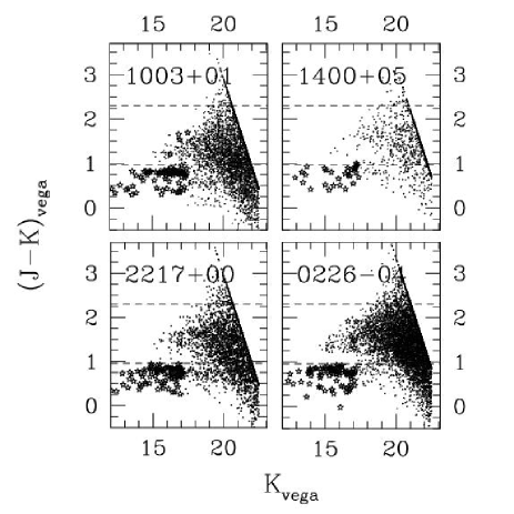
Figure 15: Colour-magnitude diagrams for the $K-$selected samples in each of our fields. The star symbols indicate objects classified as point–like using our star/galaxy classifier. See text for more details.

It is reassuring to see that the majority of objects we classified as stars are well separated from the global color distribution and are almost always below the dashed line $(J-K)=0.96$, corresponding to the typical color of a main sequence M6 star. Furthermore the stellar locus is in same position for all four fields, indicating that our absolute calibration is accurate to within $\sim 0.05$ magnitudes. In Figure 15 the dotted line at $(J-K)=2.3$ corresponds to colour of an $z\sim 2$ evolved galaxy with a prominent $4000\AA$ break as a present day elliptical, or a $z\sim 0.6$ heavily reddened starburst galaxy.

Figure 16: $(J-K)$ colour distribution for the total $K-$selected sample in different slices of $K-$band magnitude. Th¡ere is a trend towards redder colors at fainter magnitudes, probably reflecting an increasing fraction of high redshift, red, galaxies.

Figure 16 shows galaxy $(J-K)$ color distributions in different bins of $K-$band magnitudes. It is evident how the population objects red in $(J-K)$ becomes progressively important at fainter magnitudes. A detailed analysis of the number counts and clustering properties of such red population will be presented in a subsequent paper.

4.4 Clustering analysis for $K-$selected data

In this Section we investigate the clustering properties of point like and extended sources in our $K-$band catalogues.

We use the projected two-point angular correlation function, $\omega(\theta)$, which measures the excess of pairs separated by an angle $\theta,\theta+\delta\theta$ with respect to a random distribution. This statistic is useful for our purposes because it is particularly sensitive to any residual variations of the magnitude zero-point across our stacked images. We measure $\omega(\theta)$ using the standard Landy & Szalay (1993) estimator, i.e.,

$$\omega_{e}(\theta)={\mbox{DD}-2\mbox{DR}+\mbox{RR}\over\mbox{RR}}$$ (1)

with the DD, DR and RR terms referring to the number of data-data, data-random and random-random pairs between $\theta$ and $\theta+\delta\theta$. We use logarithmically spaced bins, with $\Delta log(\theta)=0.2$, and the angles are expressed in degrees, unless stated otherwise. DR and RR are obtained by populating the two-dimensional coordinate space corresponding to the different fields number of random points equal to the number of data points, a process repeated 1000 times to obtain stable mean values of these two quantities.

4.4.1 Clustering of point-like sources

We first measure the angular correlation function $\omega(\theta)$ of the stellar sources. As stars are unclustered, we expect that, if our magnitude zero-points and detection thresholds are uniform over our field, then $\omega(\theta)$ should be zero at all angular scales.

The results for $K-$band data are displayed in Figure 17, where the correlation function is plotted for the total sample of stars obtained from all fields according to the procedure described in section : 282 stars in total for the $K-$band images. At all scales displayed the measured correlation values are consistent with zero. Error bars are obtained through bootstrap resampling of the star sample (and are roughly twice poissonian error bars). A similar result is obtained for the measurement of clustering of stars obtained in $J-$band images.

Figure 17: Plot of the correlation function $\omega(\theta)$ for the total sample of stars in the $K-$band stacks as a function of the logarithm of the angular pair separation in degrees. At all scales displayed the measured correlation values are consistent with zero.

4.4.2 Clustering of extended sources

The procedure followed to measure $\omega(\theta)$ is similar to the one described above for the star sample. In the case of galaxies a positive amplitude of $\omega(\theta)$ is expected, and we have to take into account the so called “integral constraint” bias. If the real $\omega(\theta)$ is assumed to be of the form $A_{\omega}\theta^{\delta}$, our estimator (1) will be offset negatively from the true $\omega(\theta)$, according to the formula:

$$\omega_{e}(\theta)=A_{\omega}(\theta^{-\delta}-C)$$ (2)

This bias increases as the area of observation decreases, and it is caused by the need to use the observed sample itself to estimate its mean density, see eg Peebles (1980). The negative offset AC can be estimated by doubly integrating the assumed true $\omega(\theta)$ over the field area $\Omega$:

$$A_{\omega}C={1\over\Omega^{2}}\int\int\omega(\theta)d\Omega_{1}d\Omega_{2}$$ (3)

This integral can be solved numerically using randomly distributed points for each field:

$$C={\sum N_{rr}(\theta)\leavevmode\nobreak\ \theta^{-\delta}\over\sum N_{rr}(\theta)}$$ (4)

Assuming 1” as the pairs minimal scale at which two galaxies can be distinguished as separated objects, and $\delta=0.8$, we obtain the following values: $C_{0226-04}=7.58A$, $C_{2217+00}=9.31A$, $C_{1003+01}=8.60A$, $C_{1400+05}=12.64A$.

We also measured the angular correlation function for our 4 $J-$ selected galaxy samples and verified that they do not exhibit any significant deviation from a power-law within the angular separation range associated to our sample areas.

We estimated the amplitude $A_{\omega}$ for a series of $K$ limited galaxy samples by least square fitting $A(\theta^{-0.8}-C)$ to the observed $\omega(\theta)$, weighting each point using bootstrap error bars. Figure 18 shows the results obtained for each of our fields on galaxy sub-samples of different $K-$band limiting magnitudes. No correction for stellar contamination is applied (only the objects classified as stars, using the method described in section 4.4.1, were excluded from the analysis) and the error bars on the amplitude are $1\sigma$ error bars obtained from rms of the fit. The different fields are in good agreement within the error bars. The $0226-04$ field is the one with the larger area and the lower stellar contamination, and this probably explains why its amplitude values are systematically higher than those of the other fields. It should be remembered that in the presence of a randomly distributed spurious population among the sample of objects analized, like faint stars among our galaxy sample, the resulting measured correlation amplitudes are reduced by a factor $(1-f)^{2}$, where $f$ is the fraction of the randomly distributed component. Therefore a 10% (5%) contamination rate by stars implies a shifting of the values of the amplitude plotted by $\sim$ 0.1 (0.06) downwards on the y-axis. Another point to consider is the expected cosmic variance among different fields. A simple numeric estimate of the expected variation of the measured amplitude of the correlation function on the sky is $\sigma_{A}=A_{\omega}^{3/2}C^{1/2}$, see Daddi et al. (2001). For our fields the expected scatter due to cosmic variance is roughly around 10% and comparable to the scatter observed among the fields.

In Figure 18 the filled circles show our final estimate for the amplitude of the correlation function. For each limiting magnitude these values are obtained by a weighted mean of the amplitude of our four fields, and their error bars by computing the weighted variance among amplitudes (weighting proportional to the error bars on each field value).

Figure 19 shows the comparison of our results with literature data. The continous, dotted and dashed lines show the models of PLE from Roche et al. (1998), with scaling from local galaxy clustering. A more detailed analysis, involving the use of spectroscopic (from the VVDS redshift survey) and photometric redshifts for the galaxies of our sample is to be presented in a forthcoming paper.

Figure 18: Results obtained for the amplitude $A_{\omega}$ at $1\deg$ of each of our fields on galaxy sub-samples of different $K-$band limiting magnitudes. No correction for stellar contamination is applied and the error bars on the amplitude are $1\sigma$ error bars obtained from rms of the fit. The different fields show a good agreement, within the error bars. On the right of each point, slightly offset for sake of clarity, filled circles show our final estimate, from the total sample, of the amplitude of the angular correlation function.

Figure 19: We compare our total sample estimate of the amplitude, $A_{\omega}$ at $1\deg$, of the angular correlation function with a compilation of results from the literature. We include mesurements from: Daddi et al. (2000), Kümmel & Wagner (2001), McCracken et al. (2000b), Daddi et al. (2003) and Roche et al. (2003). The continous, dotted and dashed lines show, for reference, the models of PLE from Roche et al. (1998), with scaling from local galaxy clustering.

Table 6 lists our amplitude measurements for each field and for the total sample, in units of $10^{-4}$ at $1\deg$, together with their $1\sigma$ error bars, computed as explained above. For each field and limiting magnitude, the total number of objects N used in the analysis is also listed.

Magnitude	$0226-04$		$2217+00$		$1003+01$		$1400+05$		Total sample
	N	A $\pm$ dA	N	A $\pm$ dA	N	A $\pm$ dA	N	A $\pm$ dA	A $\pm$ dA
K $<$ 18.25	409	61.2 $\pm$ 15.1	234	39.8 $\pm$ 10.4	263	14.8 $\pm$ 11.4	88	51.1 $\pm$ 15.5	39.1 $\pm$ 9.5
K $<$ 18.75	670	30.2 $\pm$ 5.8	384	31.6 $\pm$ 9.9	433	17.6 $\pm$ 6.1	159	18.2$\pm$10.5	24.5 $\pm$ 3.7
K $<$ 19.25	1001	15.2 $\pm$ 4.0	611	8.9 $\pm$ 2.6	708	12.3 $\pm$ 2.9	236	12.0$\pm$ 2.3	11.6 $\pm$ 1.1
K $<$ 19.75	1458	15.1 $\pm$ 2.4	908	6.9 $\pm$ 2.3	1056	7.1 $\pm$ 4.7	343	6.7 $\pm$ 3.6	9.8 $\pm$ 2.3
K $<$ 20.25	2162	10.3 $\pm$ 2.0	1276	4.4 $\pm$ 2.4	1506	4.1 $\pm$ 3.8	488	2.1 $\pm$ 2.1	7.1 $\pm$ 1.8
K $<$ 20.75	3086	9.4 $\pm$ 1.4	1741	4.3 $\pm$ 1.5	2149	4.2 $\pm$ 3.5	709	2.8 $\pm$ 2.1	6.1 $\pm$ 1.6

Table 6: Observed $\omega(\theta)$ amplitudes A, in units of $10^{-4}$ at $1\deg$, together with their $1\sigma$ error bars, for each of our fields and for the total sample. For each field the number of objects used in the analysis down to the K magnitude faint limits shown in the first column is also listed. The number of objects in the first bin of field $1400+05$ was too small, and therefore this bin was discarded from the analysis.

5 Summary and conclusions

In this paper we have presented a new near-infrared survey covering four sub-areas located in each of the four fields of the VIMOS-VLT deep survey. We have described in detail our data reduction process starting from pre-reductions, astrometric and photometric calibrations, image resampling and stacking, and finally extraction of catalogues. At each stage, we have tried to quantify all sources of systematic and random errors in our survey. From extensive simulations, we have shown that our catalogues are reliable in all fields to at least $K\sim 20.75$ and $J\sim 21.50$: we define this limit as the magnitude where object contamination is less than 10% and completeness greater than 90%.

Based on repeated measurements of standard stars, we estimated that the error on our absolute photometric calibration, field-to-field, is $\sim 0.05\leavevmode\nobreak\$magnitudes r.m.s. This is consistent with the $\sim 5\%$ field-to-field variation of $J-$ and $K-$selected galaxy number counts and the measured field-to-field variation of the $(J-K)$ colour of the stellar locus. We separated stars from galaxies using the parameter $r_{1/2}$, which measures the radius for each object which encloses 50% of the total flux. Stellar counts for our four fields are consistent with the Robin et al. (2003) model of Milky Way, and our mean galaxy counts and counts slope over our four fields is also in excellent agreement with literature compilations. We observe a change in slope in the $K-$band galaxy number counts at $\sim 17.5$ magnitudes.

We investigated the colour-magnitude distribution of stars and galaxies identified in our catalogues. All objects lying in the $K$ vs $(J-K)$ stellar locus were successfully identified by our classifier. For the galaxy population in the range $17.5<K<20.5$ we measure a median $(J-K)$ colour of $1.4\pm 0.3$, consistent with published values. This value is remains approximately constant to progressively fainter magnitudes, until the faintest reliable limits of our sample ($20.0<K<20.5$). Our fainter magnitude slices show some evidence of a red tail of objects $(J-K)\sim 2.5$ which becomes progressively larger at fainter magnitudes.

Finally, we measure the angular clustering of stars and galaxies for our four fields. Our stellar correlation function is consistent with zero for all four fields on all angular scales. The amplitude of our galaxy correlation function shows the expected scaling behaviour for increasingly fainter magnitude slices, and is consistent previously-presented measurements.

These catalogues will be an excellent tool to investigate the properties of distant galaxies selected in the near-infrared, and such investigations which will be the subject of several forthcoming articles.

References

- Bertin & Arnouts (1996) Bertin, E. & Arnouts, S. 1996, A&AS, 117, 393
- Bertin et al. (2002) Bertin, E., Mellier, Y., Radovich, M., et al. 2002, in Astronomical Society of the Pacific Conference Series, 228–+
- Bondi et al. (2003) Bondi, M., Ciliegi, P., Zamorani, G., et al. 2003, A&A, 403, 857
- Cristóbal-Hornillos et al. (2003) Cristóbal-Hornillos, D., Balcells, M., Prieto, M., et al. 2003, ApJ, 595, 71
- Daddi et al. (2001) Daddi, E., Broadhurst, T., Zamorani, G., et al. 2001, A&A, 376, 825
- Daddi et al. (2000) Daddi, E., Cimatti, A., Pozzetti, L., et al. 2000, A&A, 361, 535
- Daddi et al. (2003) Daddi, E., Röttgering, H. J. A., Labbé, I., et al. 2003, ApJ, 588, 50
- Djorgovski et al. (1995) Djorgovski, S., Soifer, B. T., Pahre, M. A., et al. 1995, ApJ, 438, L13
- Drory et al. (2001) Drory, N., Bender, R., Snigula, J., et al. 2001, ApJ, 562, L111
- Gardner et al. (1996) Gardner, J. P., Sharples, R. M., Carrasco, B. E., & Frenk, C. S. 1996, MNRAS, 282, L1
- Huang et al. (2001) Huang, J.-S., Thompson, D., Kümmel, M. W., et al. 2001, A&A, 368, 787
- Kümmel & Wagner (2001) Kümmel, M. W. & Wagner, S. J. 2001, A&A, 370, 384
- Kron (1980) Kron, R. G. 1980, ApJS, 43, 305
- Labbé et al. (2003) Labbé, I., Franx, M., Rudnick, G., et al. 2003, AJ, 125, 1107
- Landy & Szalay (1993) Landy, S. D. & Szalay, A. S. 1993, ApJ, 412, 64
- Le Fèvre et al. (2004) Le Fèvre, O., Mellier, Y., McCracken, H. J., et al. 2004, A&A, 417, 839
- Le Fèvre et al. (2005) Le Fèvre, O. L., Vettolani, G., Garilli, B., et al. 2005, A&A, in press
- Maihara et al. (2001) Maihara, T., Iwamuro, F., Tanabe, H., et al. 2001, PASJ, 53, 25
- Martini (2001) Martini, P. 2001, AJ, 121, 598
- McCracken et al. (2000a) McCracken, H. J., Metcalfe, N., Shanks, T., et al. 2000a, MNRAS, 311, 707
- McCracken et al. (2003) McCracken, H. J., Radovich, M., Bertin, E., et al. 2003, A&A, 410, 17
- McCracken et al. (2000b) McCracken, H. J., Shanks, T., Metcalfe, N., Fong, R., & Campos, A. 2000b, MNRAS, 318, 913
- McLeod et al. (1995) McLeod, B. A., Bernstein, G. M., Rieke, M. J., Tollestrup, E. V., & Fazio, G. G. 1995, ApJS, 96, 117
- Minezaki et al. (1998) Minezaki, T., Kobayashi, Y., Yoshii, Y., & Peterson, B. A. 1998, ApJ, 494, 111
- Monet (1998) Monet, D. G. 1998, Bulletin of the American Astronomical Society, 30, 1427
- Moorwood et al. (1998) Moorwood, A., Cuby, J.-G., & Lidman, C. 1998, The Messenger, 91, 9
- Peebles (1980) Peebles, P. J. E. 1980, The large-scale structure of the universe (Princeton University Press, 1980. 435 p.)
- Persson et al. (1998) Persson, S. E., Murphy, D. C., Krzeminski, W., Roth, M., & Rieke, M. J. 1998, AJ, 116, 2475
- Radovich et al. (2004) Radovich, M., Arnaboldi, M., Ripepi, V., et al. 2004, A&A, 417, 51
- Robin et al. (2003) Robin, A. C., Reylé, C., Derrière, S., & Picaud, S. 2003, A&A, 409, 523
- Roche et al. (1998) Roche, N., Eales, S., & Hippelein, H. 1998, MNRAS, 295, 946
- Roche et al. (2003) Roche, N. D., Dunlop, J., & Almaini, O. 2003, MNRAS, 346, 803
- Sabbey et al. (2001) Sabbey, C. N., McMahon, R. G., Lewis, J. R., & Irwin, M. J. 2001, in ASP Conf. Ser. 238: Astronomical Data Analysis Software and Systems X, 317
- Saracco et al. (2001) Saracco, P., Giallongo, E., Cristiani, S., et al. 2001, A&A, 375, 1
- Schlegel et al. (1998) Schlegel, D. J., Finkbeiner, D. P., & Davis, M. 1998, ApJ, 500, 525
- Stanford et al. (1995) Stanford, S. A., Eisenhardt, P. R. M., & Dickinson, M. 1995, ApJ, 450, 512
- Szalay et al. (1999) Szalay, A. S., Connolly, A. J., & Szokoly, G. P. 1999, AJ, 117, 68
- Teplitz et al. (1999) Teplitz, H. I., McLean, I. S., & Malkan, M. A. 1999, ApJ, 520, 469
- Totani et al. (2001) Totani, T., Yoshii, Y., Maihara, T., Iwamuro, F., & Motohara, K. 2001, ApJ, 559, 592
- Wainscoat & Cowie (1992) Wainscoat, R. J. & Cowie, L. L. 1992, AJ, 103, 332