Inflation Dynamics and Reheating

Abstract

We review the theory of inflation with single and multiple fields paying particular attention to the dynamics of adiabatic and entropy/isocurvature perturbations which provide the primary means of testing inflationary models. We review the theory and phenomenology of reheating and preheating after inflation providing a unified discussion of both the gravitational and nongravitational features of multi-field inflation. In addition we cover inflation in theories with extra dimensions and models such as the curvaton scenario and modulated reheating which provide alternative ways of generating large-scale density perturbations. Finally we discuss the interesting observational implications that can result from adiabatic-isocurvature correlations and non-Gaussianity.

I Introduction

Inflation was introduced Sta80 ; Guth81 ; Sato81p1 ; Sato81p2 ; Kazanas80 as a way of addressing pressing problems that were eating away at the foundations of the otherwise rather successful big-bang model. It is a very flexible paradigm, based squarely in semi-classical physics, and has provided a sturdy foundation linking the classical cosmos and the quantum gravity world Lindebook ; LLbook ; Kolbbook .

Inflation can be viewed in many different ways. One approach is to argue that inflationary models (of which there are hundreds) provide a convenient method of parameterising the early universe but that, because they are fundamentally semi-classical, are unlikely to be a true description of the physics underlying the very early universe. The other, probably more common, approach is to argue that an inflationary phase did indeed occur at some stage in the early universe and that the source of inflation is a scalar field whose identity may be found by considering one of the extensions of the standard model based on grand unified theories (GUT’s), supergravity or string theory. In the latter view, we can use inflation as a way both to understand features of quantum gravity/string theory and of particle physics beyond the standard model.

Taking this latter view, it is extremely natural to consider inflation with many fields. As a simple example, consider a grand unified theory (GUT) based on the group $SO(10)$. Such a GUT has no pretensions to be a theory of everything and yet it already implies the existence of large numbers (of order $100$) scalar Higgs fields. Similarly supersymmetry requires the existence of large numbers of superpartners LRreview and string theory rather naturally has dynamical moduli fields corresponding to the geometrical characteristics of compactified dimensions LWCreview . If scalar fields are natural sources of inflation, then modern particle physics is the perfect supplier.

The inflationary paradigm not only provides an excellent way to solve flatness and horizon problems but also generates density perturbations as seeds for large-scale structure in the universe Mukhanov81 ; Guth82 ; Hawking82 ; Sta82 . Quantum fluctuations of the field responsible for inflation – called the inflaton – are stretched on large scales by the accelerated expansion. In the simplest version of the single-field scenario the fluctuations are “frozen” after the scale of perturbations leaves the Hubble radius during inflation. Long after the inflation ends, the perturbations cross inside the Hubble radius again. Thus inflation provides a causal mechanism for the origin of large-scale structure in the universe. An important prediction of inflation is that density perturbations generally exhibit nearly scale-invariant spectra. This prediction can be directly tested by the measurement of the temperature anisotropies in Cosmic Microwave Background (CMB). Remarkably the anisotropies observed by the Cosmic Background Explorer (COBE) in 1992 showed nearly scale-invariant spectra. Fortunately, all existing and constantly accumulating data including WMAP WMAP ; Peiris03 , SDSS Tegmark03 ; Tegmarkdata and 2dF 2dF have continued to confirm the main predictions of the inflationary paradigm within observational errors. We live in a golden age for cosmology in which the physics of the early universe can be probed from high-precision observations.

Recent progress in constructing particle-physics models of inflation has shown us that a key question is “how many light fields exist during inflation?” Here “light” is measured relative to the Hubble constant (which has dimensions of mass). If there is only one light field (typically required to get slow-roll inflation in the first place), then inflation is effectively single-field dominated and the cosmological consequences are rather well-understood. In the case of multiple light fields, the situation is significantly more complicated since the fields may interact and between each light field there will typically be a dynamically important entropy/isocurvature perturbation (we will use these two terms interchangeably).

Further, as the fields evolve, their effective mass can change, renormalised by the expectation values of other fields. Since the spectrum of fluctuations associated with any given perturbation mode depend on its effective mass, there is a rich phenomenology of possible effects associated with time-dependent effective masses.

In this review we will lay out the foundations of inflation and cosmological perturbation theory appropriate for application to cases involving many relevant fields. Our main aim is to provide the reader with a unified framework and set of tools to begin practical application in inflationary cosmology. This review is complementary to the many excellent review on related topics, given in Refs. Robert85 ; CKLLreview ; Kolbbook ; Liddle93 ; LLbook ; LLKCreview ; Lindebook ; LRreview ; Riotto02 ; NP91 ; Gio05 .

Our paper is organised as follows. In Sec. II we introduce the inflationary paradigm as a way to solve several cosmological problems associated with standard big bang cosmology. Inflationary models are classified into four different types. In Sec. III we review cosmological perturbation theory using the gauge-invariant formalism. Sec. IV is devoted to the spectra of scalar and tensor perturbations generated in single-field inflation. In Sec. V we present observational constraints on single-field inflation from CMB and galaxy redshift surveys. In Sec. VI we review density perturbations generated in higher-dimensional models including braneworld, pre-big-bang and ekpyrotic/cyclic cosmologies.

In Sec. VII the definition of adiabatic and entropy perturbations is given with the field space rotation and we show how the correlation between adiabatic and entropy perturbations emerges in the context of two-field inflation. In Sec. VIII we present general features in the CMB from correlations. In Sec. IX we explain the elementary theory of reheating after inflation. Sec. X is devoted to preheating in which particles coupled to the inflaton are resonantly amplified by parametric resonance. In Sec. XI we discuss the evolution of metric perturbations during preheating and possible consequences from it. We review the curvaton scenario in Sec. XII and the modulated reheating scenario in Sec. XIII to generate large-scale density perturbations as alternative models of inflation. Summary and future outlook are given in the final section.

II Dynamics of inflation

II.1 The standard big-bang cosmology

The standard big-bang cosmology is based upon the cosmological principle LLbook , which requires that the universe is homogeneous and isotropic on averaging over large volumes. Then the metric takes the Friedmann-Robertson-Walker (FRW) form:

$${\rm d}s^{2} = g_{\mu\nu}{\rm d}x^{\mu}{\rm d}x^{\nu}$$ (1)

$$= -{\rm d}t^{2}+a^{2}\left[\frac{{\rm d}r^{2}}{1-Kr^{2}}+r^{2}({\rm d}\theta^{2}+\sin^{2}\theta{\rm d}\phi^{2})\right].$$

Here $a(t)$ is the scale factor with $t$ being the cosmic time. The constant $K$ is the spatial curvature, where positive, zero, and negative values correspond to closed, flat, and hyperbolic spatial sections respectively.

The evolution of the universe is dependent on the material within it with a key role played by the equation of state relating the energy density $\rho(t)$ and the pressure $P(t)$. For example we have

$$P = \rho/3\,,~{}~{}~{}~{}~{}~{}{\rm radiation}\,,$$ (2)

$$P = 0\,,~{}~{}~{}~{}~{}~{}~{}~{}~{}{\rm dust}\,.$$ (3)

The dynamical evolution of the universe is known once we solve the Einstein equations of General Relativity:

$$G_{\mu\nu}\equiv R_{\mu\nu}-\frac{1}{2}g_{\mu\nu}R=8\pi GT_{\mu\nu}-\Lambda g_{\mu\nu},$$ (4)

where $R_{\mu\nu}$, $R$, $T_{\mu\nu}$, and $G$ are the Ricci tensor, Ricci scalar, energy-momentum tensor and gravitational constant, respectively. The Planck energy, $m_{\rm pl}=1.2211\times 10^{19}$ GeV, is related to $G$ through the relation $m_{\rm pl}=(\hbar c^{5}/G)^{1/2}$. Here $\hbar$ and $c$ are the Planck’s constant and the speed of light, respectively. Hereafter we use the units $\hbar=c=1$. $\Lambda$ is the cosmological constant originally introduced by Einstein to make the universe static. In what follows we set the cosmological constant to zero ($\Lambda=0$) unless otherwise stated, preferring to include any non-zero vacuum energy density in the total energy-momentum tensor.

From the Einstein equations (4) for the background FRW metric (1), we obtain the field equations:

$$H^{2}=\frac{8\pi}{3m_{\rm pl}^{2}}\rho-\frac{K}{a^{2}}\,,$$ (5)

$$\frac{\ddot{a}}{a}=-\frac{4\pi}{3m_{\rm pl}^{2}}(\rho+3P)\,,$$ (6)

where a dot denotes the derivative with respect to $t$, and $H\equiv\dot{a}/a$ is the Hubble expansion rate. Eqs. (5) and (6) are the Friedmann and Raychaudhuri equations, respectively. Combining these relations implies energy conservation,

$$\dot{\rho}+3H(\rho+P)=0\,,$$ (7)

which is known as the continuity or fluid equation.

The Friedmann equation (5) can be rewritten as

$$\Omega-1=\frac{K}{a^{2}H^{2}}\,,$$ (8)

where

$$\Omega\equiv\frac{\rho}{\rho_{c}},~{}~{}~{}{\rm with}~{}~{}~{}\rho_{c}\equiv\frac{3H^{2}m_{\rm pl}^{2}}{8\pi}\,.$$ (9)

Here the density parameter $\Omega$ is the ratio of the energy density to the critical density. When the spatial geometry is flat ($K=0$; $\Omega=1$), the solutions for Eqs. (5) and (7) are

$${\rm Radiation}:~{}~{}a\propto t^{1/2}\,,~{}~{}~{}\rho\propto a^{-4}\,,$$ (10)

$${\rm Dust}:~{}~{}a\propto t^{2/3}\,,~{}~{}~{}\rho\propto a^{-3}\,.$$ (11)

In these simple cases, the universe exhibits a decelerated expansion ($\ddot{a}<0$) as confirmed by Eq. (6).

II.2 Problems of the standard big-bang cosmology

II.2.1 Flatness problem

In the standard big-bang theory with $\ddot{a}<0$, the $a^{2}H^{2}(=\dot{a}^{2})$ term in Eq. (8) always decreases. This means that $\Omega$ tends to evolve away from unity with the expansion of the universe. However, since present observations suggest that $\Omega$ is within a few percent of unity today WMAP , $\Omega$ is forced to be much closer to unity in the past. For example, we require $|\Omega-1|<{\cal O}(10^{-16})$ at the epoch of nucleosynthesis and $|\Omega-1|<{\cal O}(10^{-64})$ at the Planck epoch LLbook . This appears to be an extreme fine-tuning of initial conditions. Unless initial conditions are chosen very accurately, the universe either collapses too soon, or expands too quickly before the structure can be formed. This is the so-called flatness problem.

II.2.2 Horizon problem

Consider a comoving wavelength, $\lambda$, and corresponding physical wavelength, $a\lambda$, which at some time is inside the Hubble radius, $H^{-1}$ (i.e., $a\lambda~{}\mbox{\raisebox{-4.30554pt}{$\stackrel{{\scriptstyle\textstyle<}}{{\textstyle\sim}}$}}~{}H^{-1}$). The standard big-bang decelerating cosmology is characterized by the cosmic evolution of $a\propto t^{n}$ with $0<n<1$. In this case the physical wavelength grows as $a\lambda\propto t^{n}$, whereas the Hubble radius evolves as $H^{-1}\propto t$. Therefore the physical wavelength becomes much smaller than the Hubble radius at late times. Conversely any finite comoving scale becomes much larger than the Hubble scale at early times. This means that a causally connected region can only be a small fraction of the Hubble radius.

To be more precise, let us first define the particle horizon $D_{H}(t)$ which is the distance travelled by light since the beginning of the universe, at time $t_{*}$,

$$D_{H}(t)=a(t)d_{H}(t)\,,~{}~{}~{}{\rm with}~{}~{}~{}d_{H}(t)=\int_{t_{*}}^{t}\frac{{\rm d}t^{\prime}}{a(t^{\prime})}\,.$$ (12)

Here $d_{H}(t)$ corresponds to the comoving particle horizon. Setting $t_{*}=0$, we find $D_{H}(t)=3t$ in the matter-dominant era and $D_{H}(t)=2t$ in an early hot big bang. We observe photons in the cosmic microwave background (CMB) which are last-scattered at the time of decoupling. The particle horizon at decoupling, $D_{H}(t_{\rm dec})=a(t_{\rm dec})d_{H}(t_{\rm dec})$, corresponds to the causally connected region at that time. The ratio of the comoving particle horizon at decoupling, $d_{H}(t_{\rm dec})$, to the particle horizon today, $d_{H}(t_{0})$, can be estimated to be

$$\frac{d_{H}(t_{\rm dec})}{d_{H}(t_{0})}\approx\left(\frac{t_{\rm dec}}{t_{0}}\right)^{1/3}\approx\left(\frac{10^{5}}{10^{10}}\right)^{1/3}\approx 10^{-2}.$$ (13)

This implies that the causally connected regions at last scattering are much smaller than the horizon size today. In fact causally connected regions on the surface of last scattering corresponds to an angle of order $1^{\circ}$.

This appears to be at odds with observations of the cosmic microwave background (CMB) which has the same temperature to high precision in all directions on the CMB sky. Yet there is no way to establish thermal equilibrium if these points were never been in causal contact before last-scattering. This is the so-called horizon problem.

II.2.3 The origin of large-scale structure in the universe

Experiments which observe temperature anisotropies in the CMB find that the amplitude of the anisotropies is small and their power spectrum is close to scale-invariant on large scales WMAP . These fluctuations are distributed on such a large scale that it is impossible to generate them via causal processes in a FRW metric in the time between the big bang and the time of the last scattering. Hence, standard big-bang models can neither explain the FRW metric nor explain the deviations from FRW if a FRW background is assumed.

II.2.4 Relic density problem

The standard paradigm of modern particle physics is that physical laws were simpler in the early universe before gauge symmetries were broken. The breaking of such symmetries leads to the production of many unwanted relics such as monopoles, cosmic strings, and other topological defects Lindebook . The existence of a finite horizon size leads to a maximum causal correlation length during any symmetry breaking transition and hence gives a lower bound on the density of defects. In particular, any grand unified theory based on a simple Lie group that includes the $U(1)$ of electromagnetism must produce monopoles. String theories also predict supersymmetric particles such as gravitinos, Kaluza-Klein particles, and weakly coupled moduli fields.

If these massive particles exist in the early stages of the universe then their energy densities decrease as a matter component ($\propto a^{-3}$) once the temperature drops below their rest mass. Since the radiation energy density decreases $\propto a^{-4}$, these massive relics if they are stable (or sufficiently long-lived) could become the dominant matter in the early universe depending on their number density and therefore contradict a variety of observations such as those of the light element abundances. This problem is known as the relic density problem.

II.3 Idea of inflationary cosmology

The problems in the standard big bang cosmology lie in the fact that the universe always exhibits decelerated expansion. Let us assume instead the existence of a stage in the early universe with an accelerated expansion of the universe, i.e.,

$$\ddot{a}>0\,.$$ (14)

From the relation (6) this gives the condition

$$\rho+3P<0\,,$$ (15)

which corresponds to violating the strong energy condition. The condition (14) essentially means that $\dot{a}\,(=aH)$ increases during inflation and hence that the comoving Hubble radius, $(aH)^{-1}$, decreases in the inflationary phase. This property is the key point to solve the cosmological puzzles in the standard big-bang cosmology.

II.3.1 Flatness problem

Since the $a^{2}H^{2}$ term in Eq. (8) increases during inflation, $\Omega$ is rapidly driven towards unity. After the inflationary period ends, the evolution of the universe is followed by the conventional big-bang phase and $|\Omega-1|$ begins to increase again. But as long as the inflationary expansion lasts sufficiently long and drives $\Omega$ very close to one, $\Omega$ will remain close to unity even in the present epoch.

II.3.2 Horizon problem

Since the scale factor evolves approximately as $a\propto t^{n}$ with $n>1$ during inflation, the physical wavelength, $a\lambda$, grows faster than the Hubble radius, $H^{-1}(\propto t)$. Therefore physical wavelengths are pushed outside the Hubble radius during inflation which means that causally connected regions can be much larger than the Hubble radius, thus potentially solving the horizon problem. Formally the particle horizon, defined in Eq. (12) diverges as $a(t_{*})\to 0$ in an inflationary universe.

Of course the Hubble radius begins to grow faster than the physical wavelength after inflation ends, during the subsequent radiation and matter dominant eras. In order to solve the horizon problem, it is required that the following condition is satisfied for the comoving particle horizon:

$$\int_{t_{*}}^{t_{\rm dec}}\frac{{\rm d}t}{a(t)}\gg\int_{t_{\rm dec}}^{t_{0}}\frac{{\rm d}t}{a(t)}\,.$$ (16)

This implies that the comoving distance that photons can travel before decoupling needs to be much larger than that after the decoupling. A detailed calculation shows this is achieved when the universe expands at least about $e^{70}$ times during inflation, or $70$ e-folds of expansion Lindebook ; LLbook ; Riotto02 .

II.3.3 The origin of the large-scale structure

The fact that the Hubble rate, $H(t)$, is almost constant during inflation means that it is possible to generate a nearly scale-invariant density perturbation on large scales. Since the scales of perturbations are well within the Hubble radius in the early stage of inflation, causal physics works to generate small quantum fluctuations. On very small scales we can neglect the cosmological expansion and perturbations can be treated as fluctuations in flat spacetime. But after a scale is pushed outside the Hubble radius (i.e., the first Hubble radius crossing) during inflation, we can no longer neglect the Hubble expansion.

Fluctuations in a light field become over-damped on long-wavelengths, leading to a squeezed state in phase-space, so that the perturbations can effectively be described as classical on these large scales. When the inflationary period ends, the evolution of the universe follows the standard big-bang cosmology, and the comoving Hubble radius begins to increase until the scales of perturbations cross inside the Hubble radius again (the second Hubble radius crossing). The small perturbations imprinted during inflation have amplitudes determined by the Hubble rate which is approximately constant and hence leads to an almost scale-invariant spectrum with constant amplitude on different scales. In this way the inflationary paradigm naturally provides a causal mechanism to generate the seeds of density perturbations observed in the CMB anisotropies.

II.3.4 Relic density problem

During the inflationary phase ($\rho+3P<0$), the energy density of the universe decreases very slowly. For example, when the universe evolves as $a\propto t^{n}$ with $n>1$, we have $H\propto t^{-1}\propto a^{-1/n}$ and $\rho\propto a^{-2/n}$. Meanwhile the energy density of massive particles decreases much faster ($\propto a^{-3}$), and these particles are red-shifted away during inflation, thereby solving the monopole problem, as long as the symmetry breaking transition that produces the monopoles occurs at least 20 or so e-foldings before the end of inflation.

We also have to worry about the possibility of producing these unwanted particles after inflation. In the process of reheating followed by inflation, the energy of the universe can be transferred to radiation or other light particles. At this stage unwanted particles must not be overproduced in order not to violate the success of the standard cosmology such as nucleosynthesis. Generally if the reheating temperature at the end of inflation is sufficiently low, the thermal production of unwanted relics such as gravitinos can be avoided KM95 ; moroi95 .

II.4 Inflationary dynamics

Scalar fields are fundamental ingredients in modern theories of particle physics. We will consider a homogeneous single scalar field, $\phi$, called the inflaton, whose potential energy can lead to the accelerated expansion of the universe. Neglecting spatial gradients, the energy density and the pressure of the inflaton are given by

$$\rho=\frac{1}{2}\dot{\phi}^{2}+V(\phi)\,,~{}~{}~{}P=\frac{1}{2}\dot{\phi}^{2}-V(\phi)\,,$$ (17)

where $V(\phi)$ is the potential energy of the inflaton. Substituting Eq. (17) into Eqs. (5) and (7), we obtain

$$H^{2}=\frac{8\pi}{3m_{\rm pl}^{2}}\left[\frac{1}{2}\dot{\phi}^{2}+V(\phi)\right]\,,$$ (18)

$$\ddot{\phi}+3H\dot{\phi}+V_{\phi}(\phi)=0\,,$$ (19)

where $V_{\phi}\equiv{\rm d}V/{\rm d}\phi$. The curvature term, $K^{2}/a^{2}$, is dropped in Eq. (18) since it adds nothing concrete to our discussion.

The condition for inflation (15) requires $\dot{\phi}^{2}<V(\phi)$ or classically that the potential energy of the inflaton dominates over the kinetic energy. Hence one requires a sufficiently flat potential for the inflaton in order to lead to sufficient inflation. Imposing the slow-roll conditions: $\dot{\phi}^{2}/2\ll V(\phi)$ and $|\ddot{\phi}|\ll 3H|\dot{\phi}|$, Eqs. (18) and (19) are approximately given as

$$H^{2}\simeq\frac{8\pi V(\phi)}{3m_{\rm pl}^{2}}\,,$$ (20)

$$3H\dot{\phi}\simeq-V_{\phi}(\phi)\,.$$ (21)

One can define the so-called slow-roll parameters

$$\epsilon=\frac{m_{\rm pl}^{2}}{16\pi}\left(\frac{V_{\phi}}{V}\right)^{2}\,,~{}\eta=\frac{m_{\rm pl}^{2}V_{\phi\phi}}{8\pi V}\,,~{}\xi^{2}=\frac{m_{\rm pl}^{4}V_{\phi}V_{\phi\phi\phi}}{64\pi^{2}V^{2}}\,.$$ (22)

We can easily verify that the above slow-roll approximations are valid when $\epsilon\ll 1$ and $|\eta|\ll 1$ for a prolonged period of time.

The inflationary phase ends when $\epsilon$ and $|\eta|$ grow to of order unity, though this does not, of itself, imply reheating of the universe. A useful quantity to describe the amount of inflation is the number of e-foldings, defined by

$$N\equiv\ln\frac{a_{f}}{a}=\int_{t}^{t_{f}}H{\rm d}t\simeq\frac{8\pi}{m_{\rm pl}^{2}}\int_{\phi_{f}}^{\phi}\frac{V}{V_{\phi}}{\rm d}\phi\,,$$ (23)

where the subscript $f$ denotes evaluation of the quantity at the end of inflation.

In order to solve the flatness problem, $\Omega$ is required to be $|\Omega_{f}-1|~{}\mbox{\raisebox{-4.30554pt}{$\stackrel{{\scriptstyle\textstyle<}}{{\textstyle\sim}}$}}~{}10^{-60}$ right after the end of inflation. Meanwhile the ratio $|\Omega-1|$ between the initial and final phase of slow-roll inflation is given by

$$\frac{|\Omega_{f}-1|}{|\Omega_{i}-1|}\simeq\left(\frac{a_{i}}{a_{f}}\right)^{2}=e^{-2N_{i}}\,,$$ (24)

where we used the fact that $H$ is nearly constant during slow-roll inflation. Assuming that $|\Omega_{i}-1|$ is of order unity, the number of e-foldings is required to be $N~{}\mbox{\raisebox{-4.30554pt}{$\stackrel{{\scriptstyle\textstyle>}}{{\textstyle\sim}}$}}~{}60$ to solve the flatness problem. This statement is a statement about the measure on the space of initial conditions and is therefore properly in the domain of quantum gravity. It is clear that for any fixed number of e-foldings one can choose an infinite number of $\Omega_{i}$ such that the flatness problem is not solved. Nevertheless, inflation certainly mitigates the problem. We require a similar number of e-foldings in order to solve the horizon problem and hence $N>60$ is taken as a standard target minimum number of e-foldings for any new model of inflation.

II.5 Models of inflation

So far we have not discussed the form of the inflaton potential, $V(\phi)$. The original “old inflation” scenario Guth81 ; Sato81p1 ; Sato81p2 assumed the inflaton was trapped in a metastable false vacuum and had to exit to the true vacuum via a first-order transition. As Guth pointed out Guth81 this could occur neither gracefully nor completely, problems avoided in the “new inflation” model where inflation ends via a second-order phase transition after a phase of slow roll. We now have many varieties of inflationary models : $R^{2}$, new, chaotic, extended, power-law, hybrid, natural, supernatural, extra-natural, eternal, D-term, F-term, brane, oscillating, trace-anomaly driven, k, ghost, tachyon,…, etc…

The different kinds of single-field inflationary models can be roughly classified in the following way Kolb99 . The first class (type I) consists of the “large field” models, in which the initial value of the inflaton is large and it slow rolls down toward the potential minimum at smaller $\phi$. Chaotic inflation Linde83 is one of the representative models of this class. The second class (type II) consists of the “small field” models, in which the inflaton field is small initially and slowly evolves toward the potential minimum at larger $\phi$. New inflation Linde82 ; Albre82 and natural inflation Freese90 are the examples of this type. In the first class one usually has $V_{\phi\phi}>0$, whereas it can change the sign in the second class. The third class (type III) consists of the hybrid inflation models Linde94 , in which inflation typically ends by a phase transition triggered by the presence of a second scalar field. The fourth class (type IV) consists of the double inflation models in which there exist two dynamical scalar fields leading to the two stage of inflation. A simple example is two light massive scalar fields given in Ref. Polarski92 .

We note that several models of inflation can not be classified in the above four classes. For example, some models do not have a potential minimum such as quintessential inflation PV99 and tachyon inflation FT02 ; Fe02 ; Paddy02 ; PST05 ; Sami02 ; SCQ02 ; TW05 . Typically these scenarios suffer from a reheating problem Kofman02 , since gravitational particle production is not efficient compared to the standard non-gravitational particle production by an oscillating inflaton field. There exist other models of inflation in which an accelerated expansion is realised without using the potential of the inflaton. For example, k-inflation Picon99 and ghost inflation Arkani03 belong to this class. In this case inflation occurs in the presence of higher-order kinematic terms of a scalar field. Inflation can also be realised when the higher-order curvature terms are present Sta80 ; MO04 ; CTS05 ; NOZ00 ; NO00 ; NO03 ; HHR01 ; ellis99 ; BB89 , even without an inflaton potential. Apart from these models, let us briefly review each class of inflationary models.

II.5.1 Large-field models

The large-field models are typically characterized by the monomial potential

$$V(\phi)=V_{0}\phi^{n}\,.$$ (25)

The quadratic and quartic potentials in chaotic inflation correspond to $n=2$ and $n=4$, with inflation occurring for Planckian scale values of $\phi$ (see Fig. 1). Such models lend themselves naturally to randomly distributed initial conditions with regions of spacetime that initially have $\phi>m_{\rm pl}$ and are homogeneous on the Hubble scale undergoing inflation and therefore potentially giving rise to our observable universe Lindebook .

It is easy to get analytic forms of solutions under the slow-roll approximation: $\epsilon\ll 1$ and $|\eta|\ll 1$. For example in the case of the quadratic potential ($n=2$ and $V_{0}=m^{2}/2$) we get the following relation by Eqs. (20) and (21):

$$\phi\simeq\phi_{i}-\frac{mm_{\rm pl}}{2\sqrt{3\pi}}t\,,$$ (26)

$$a\simeq a_{i}\exp\left[2\sqrt{\frac{\pi}{3}}\frac{m}{m_{\rm pl}}\left(\phi_{i}t-\frac{mm_{\rm pl}}{4\sqrt{3\pi}}t^{2}\right)\right],$$ (27)

where $\phi_{i}$ is an integration constant corresponding to the initial value of the inflaton. The relation (27) implies that the universe expands exponentially during the initial stage of inflation. The expansion rate slows down with the increase of the second term in the square bracket of Eq. (27). We require the condition, $\phi_{i}~{}\mbox{\raisebox{-4.30554pt}{$\stackrel{{\scriptstyle\textstyle>}}{{\textstyle\sim}}$}}~{}3m_{\rm pl}$, in order to have the number of e-foldings which is larger than $N=60$.

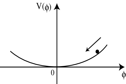
Figure 1: Schematic illustration of the potential of large-field models.

II.5.2 Small-field models

The small-field models are characterized by the following potential around $\phi=0$:

$$V(\phi)=V_{0}\left[1-\left(\frac{\phi}{\mu}\right)^{n}\right]\,,$$ (28)

which may arise in spontaneous symmetry breaking. The potential (28) corresponds to a Taylor expansion about the origin, but realistic small-field models also have a potential minimum at some $\phi\neq 0$ to connect to the reheating stage.

For example let us consider natural inflation model in which a Pseudo Nambu-Goldstone boson (PNGB) plays the role of inflaton. The PNGB potential is expressed as Freese90

$$V(\phi)=m^{4}\left[1+\cos\left(\frac{\phi}{f}\right)\right]\,,$$ (29)

where two mass scales $m$ and $f$ characterize the height and width of the potential, respectively (see Fig. 2). The typical mass scales for successful inflation are of order $f\sim m_{\rm pl}\sim 10^{19}$ GeV and $m\sim m_{\rm GUT}\sim 10^{16}$ GeV. The potential (29) has a minimum at $\phi=\pi f$.

One typical property in the type II model is that the second derivative of the inflaton potential can change sign. In natural inflation $V_{\phi\phi}$ is negative when inflaton evolves in the region of $0<\phi<\pi f/2$. This leads to the enhancement of inflaton fluctuations by spinodal (tachyonic) instability Cormier99 ; Cormier00 ; Tsujispi ; Felder01p1 ; Felder01p2 . When the particle creation by spinodal instability is neglected, the number of e-foldings is expressed by

$$N=\frac{16\pi f^{2}}{m_{\rm pl}^{2}}{\rm ln}\left[\frac{\sin(\phi_{f}/2f)}{\sin(\phi_{i}/2f)}\right]\,.$$ (30)

In order to achieve a sufficient number of e-foldings ($N~{}\mbox{\raisebox{-4.30554pt}{$\stackrel{{\scriptstyle\textstyle>}}{{\textstyle\sim}}$}}~{}60$), the initial value of the inflaton is required to be $\phi_{i}~{}\mbox{\raisebox{-4.30554pt}{$\stackrel{{\scriptstyle\textstyle<}}{{\textstyle\sim}}$}}~{}0.1m_{\rm pl}$ for the mass scale $f\sim m_{\rm pl}$.

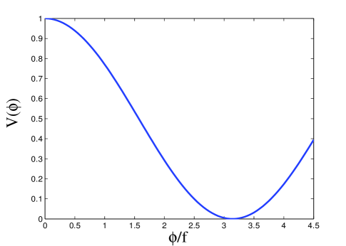
Figure 2: The schematic illustration of the potential of small-field models.

II.5.3 Hybrid inflation

Hybrid inflation models involve more than one scalar field. This scenario is particularly motivated from the viewpoint of particle physics Cope94 ; LRreview ; Linde97b . Inflation continues from an initial large value of the inflaton which decreases until it reaches a bifurcation point, after which the field becomes unstable and undergoes a “waterfall” transition towards a global minimum (see Fig. 3). During the initial inflationary phase the potential of the hybrid inflation is effectively described by a single field:

$$V(\phi)=V_{0}\left[1+\left(\frac{\phi}{\mu}\right)^{n}\right]\,.$$ (31)

Consider the Linde hybrid inflation model with potential Linde94

$$V=\frac{\lambda}{4}\left(\chi^{2}-\frac{M^{2}}{\lambda}\right)^{2}+\frac{1}{2}g^{2}\phi^{2}\chi^{2}+\frac{1}{2}m^{2}\phi^{2}\,.$$ (32)

When $\phi^{2}$ is large the field rolls down toward the potential minimum at $\chi=0$. Then we have

$$V\simeq\frac{M^{4}}{4\lambda}+\frac{1}{2}m^{2}\phi^{2}\,.$$ (33)

The mass-squared of $\chi$ becomes negative for $\phi<\phi_{c}\equiv M/g$ signifying a tachyonic instability. Then the field begins to roll down to one of the true minima at $\phi=0$ and $\chi=\pm M/\sqrt{\lambda}$ (and thereby creates domain walls). In this original version of the hybrid inflation Linde94 inflation soon comes to an end after the symmetry breaking ($\phi<\phi_{c}$) due to the rapid rolling of the field $\chi$. In this case the number of e-foldings can be approximately estimated by using the potential (33):

$$N\simeq\frac{2\pi M^{4}}{\lambda m^{2}m_{\rm pl}^{2}}\,{\rm ln}\frac{\phi_{i}}{\phi_{c}}\,,$$ (34)

where $\phi_{i}$ is the initial value of inflaton.

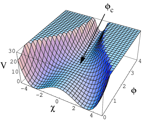
Figure 3: Schematic illustration of the potential of hybrid (or double) inflation models given by Eq. (32). Here $\phi_{c}$ is the critical value of the inflaton below which $\chi=0$ becomes unstable due to tachyonic instability ($m_{\chi}^{2}<0$).

II.5.4 Double inflation

Double inflation can occur even for the potential (32) depending on the model parameters. When the condition, $M^{2}\gg\lambda m_{\rm pl}^{2}$, is satisfied, the mass of the field $\chi$ is “light” relative to the Hubble rate around $\phi=\phi_{c}$, thereby leading to a second stage of inflation for $\phi<\phi_{c}$ Randall96 ; Garcia96hybrid ; Tsuji03 . This corresponds to a genuine multi-field inflationary model, with more than one light field, of the type that we will examine in later sections. More generally multi-field inflation may be naturally realised near points of enhanced symmetry in moduli space Kadota03 ; Kadota03v2 . In any model where more than one scalar field is light during inflation then there is no longer a unique attractor trajectory in phase-space and such models can support isocurvature as well as adiabatic perturbations about a particular background solution.

An alternative form of double inflation is also realised in the following simple model:

$$V(\phi,\chi)=\frac{1}{2}m_{\phi}^{2}\phi^{2}+\frac{1}{2}m_{\chi}^{2}\chi^{2}\,,$$ (35)

as studied by Polarski and Starobinsky Polarski92 , and later by Langlois Langlois99 who realised that the adiabatic and isocurvature perturbations surviving at the end of inflation will in general be correlated.

III Cosmological perturbations

Having undertaken a rapid tour of standard inflationary theory and models we move to discussion of perturbations. The description of the Universe as a perfectly homogeneous and isotropic FRW model is obviously an idealisation. In practice we are interested in deviations from homogeneity and isotropy that enable us to characterise different models. We will deal with small perturbations, but we will assume that the distribution of perturbations is statistically homogeneous and isotropic, which is an alternative statement of the Copernican principle.

In particular we have so far considered only the dynamics of homogeneous scalar fields driving inflation. But to investigate inflation models in more detail, and to test theoretical predictions against cosmological observations we need to consider inhomogeneous perturbations. In this section we will define the variables and notation used in subsequent sections to describe cosmological perturbations generated by inflation.

We will consider only small perturbations about the homogeneous fields

$$\phi=\phi_{0}(t)+\delta\phi(t,x)\,,$$ (36)

and only keep terms to first-order in $\delta\phi$.

III.1 Metric perturbations

For an inhomogeneous matter distribution the Einstein equations imply that we must also consider inhomogeneous metric perturbations about the spatially flat FRW metric. The perturbed FRW spacetime is described by the line element

$${\rm d}s^{2} = -(1+2A){\rm d}t^{2}+2a(\partial_{i}B-S_{i}){\rm d}x^{i}{\rm d}t$$

$$+a^{2}\left[(1-2\psi)\delta_{ij}+2\partial_{ij}E+2\partial_{(i}F_{j)}+h_{ij}\right]{\rm d}x^{i}{\rm d}x^{j}\,,$$

where $\partial_{i}$ denotes the spatial partial derivative $\partial/\partial x^{i}$. We will use lower case latin indices to run over the 3 spatial coordinates. Our metric perturbations follow the notation of Ref. Mukhanov90 , apart from our use of $A$ rather than $\phi$ as the perturbation in the lapse function.

The metric perturbations have been split into scalar, vector and tensor parts according to their transformation properties on the spatial hypersurfaces. The Einstein equations for the scalar, vector and tensor parts then decouple to linear order. We do not consider second-order cosmological perturbations in this review Acqu03 .

III.1.1 Scalar perturbations

The four scalar metric perturbations $A$, $\partial_{i}B$, $\psi\delta_{ij}$ and $\partial_{ij}E$ are constructed from 3-scalars, their derivatives, and the background spatial metric. The intrinsic Ricci scalar curvature of constant time hypersurfaces is given by

$${}^{(3)}R=\frac{4}{a^{2}}\nabla^{2}\psi\,,$$ (38)

where $\nabla^{2}\equiv\delta^{ij}\partial_{ij}$ is the spatial Laplacian, and hence we refer to $\psi$ as the curvature perturbation. We can Fourier decompose an arbitrary scalar perturbation with respect to the complete set of eigenvectors of the spatial Laplacian, $\nabla^{2}\psi=-k^{2}\psi$, with comoving wavenumber $k$ indexing the corresponding eigenvalues.

Under a scalar coordinate/gauge transformation

$$t \to t+\delta t\,,$$ (39)

$$x^{i} \to x^{i}+\delta^{ij}\partial_{j}\delta x\,,$$ (40)

$\delta t$ determines the time slicing and $\delta x$ the spatial threading. The scalar metric perturbations then transform as

$$A \to A-\dot{\delta t}\,,$$ (41)

$$B \to B+a^{-1}\delta t-a\dot{\delta x}\,,$$ (42)

$$E \to E-\delta x\,,$$ (43)

$$\psi \to \psi+H\delta t\,.$$ (44)

Although $B$ and $E$ separately are spatially gauge-dependent, the combination $\dot{E}-B/a$ is independent of spatial gauge and describes the scalar potential for the anisotropic shear of worldlines orthogonal to constant time hypersurfaces Kodama84 .

We can construct a variety of gauge-invariant combinations of the scalar metric perturbations. The longitudinal gauge corresponds to a specific gauge-transformation to a (zero-shear) frame such that $E=B=0$, leaving the gauge-invariant variables

$$\Phi \equiv A-\frac{{\rm d}}{{\rm d}t}\left[a^{2}(\dot{E}-B/a)\right]\,,$$ (45)

$$\Psi \equiv \psi+a^{2}H(\dot{E}-B/a)\,.$$ (46)

Matter perturbations are also gauge-dependent. Scalar field, density and pressure perturbations all obey the simple transformation rule

$$\delta\rho\to\delta\rho-\dot{\rho}\delta t\,.$$ (47)

The adiabatic pressure perturbation is defined to be

$$\delta P_{\rm ad}\equiv\frac{\dot{P}}{\dot{\rho}}\delta\rho\,,$$ (48)

and hence the non-adiabatic part of the actual pressure perturbation, or entropy perturbation, is a gauge-invariant perturbation

$$\delta P_{\rm nad}=\delta P-\frac{\dot{P}}{\dot{\rho}}\delta\rho\,.$$ (49)

The scalar part of the 3-momentum is given by $\partial_{i}\delta q$ and this momentum potential transforms as

$$\delta q\to\delta q+(\rho+P)\delta t\,.$$ (50)

Thus we can obtain the gauge-invariant comoving density perturbation Bardeen80

$$\delta\rho_{m}=\delta\rho-3H\delta q\,.$$ (51)

We can construct two further commonly used gauge-invariant combinations in terms of matter and metric perturbations. The curvature perturbation on uniform-density hypersurfaces is given by

$$-\zeta\equiv\psi+\frac{H}{\dot{\rho}}\delta\rho\,,$$ (52)

first defined by Bardeen, Steinhardt and Turner Bardeen83 (see also Refs. Bardeen88 ; Martin98 ; Wands00 ). The comoving curvature perturbation (strictly speaking the curvature perturbation on hypersurfaces orthogonal to comoving worldlines)

$${\cal R}\equiv\psi-\frac{H}{\rho+P}\delta q\,.$$ (53)

This has been used by Lukash Lukash80 , Lyth Lyth85 and many others, including Mukhanov, Feldman and Brandenberger in their review Mukhanov90 . (Note that in their review the comoving curvature perturbation is denoted by “$\zeta$” in Ref. Mukhanov90 and defined in terms of the metric perturbations in the longitudinal gauge, but it is equivalent to our definition of ${\cal R}$ in a spatially flat background with vanishing anisotropic stress.) The difference between the two curvature perturbations ${\cal R}$ and $-\zeta$ is proportional to the comoving density perturbation:

$$-\zeta={\cal R}+\frac{H}{\dot{\rho}}\delta\rho_{m}\,.$$ (54)

For single field inflation we have $\delta q=-\dot{\phi}\delta\phi$ and hence

$${\cal R}\equiv\psi+\frac{H}{\dot{\phi}}\delta\phi\,.$$ (55)

In slow-roll single-field inflation we have $\delta\rho/\dot{\rho}\simeq\delta\phi/\dot{\phi}$ and hence $\delta\rho_{m}\simeq 0$ and these two commonly used curvature perturbations, ${\cal R}$ and $-\zeta$, coincide.

Finally we note that another variable commonly used to describe scalar perturbations during inflation is the field perturbation in the spatially flat gauge (where $\psi=0$). This has the gauge-invariant definition Mukhanov85 ; Sasaki86 :

$$\delta\phi_{\psi}\equiv\delta\phi+\frac{\dot{\phi}}{H}\psi\,.$$ (56)

In single field inflation this is simply a rescaling of the comoving curvature perturbation ${\cal R}$ in (53). We see that what appears as a field perturbation in one gauge is a metric perturbation in another gauge and vice versa.

III.1.2 Vector perturbations

The vector perturbations $S_{i}$ and $F_{i}$ can be distinguished from scalar perturbations as they are solenoidal (divergence-free), i.e., $\partial^{i}S_{i}=0$.

Under a vector coordinate/gauge transformation

$$x^{i} \to x^{i}+\delta x^{i}\,,$$ (57)

the vector metric perturbations transform as

$$S_{i} \to S_{i}+a\dot{\delta x}_{i}\,,$$ (58)

$$F_{i} \to F_{i}-\delta x_{i}\,,$$ (59)

and hence $\dot{F}_{i}+S_{i}/a$ is the gauge-invariant vector shear perturbation.

III.1.3 Tensor modes

The tensor perturbations $h_{ij}$ are transverse $\partial^{i}h_{ij}=0$ and trace-free $\delta^{ij}h_{ij}=0$. They are automatically independent of coordinate gauge transformations.

These are referred to as gravitational waves as they are the free part of the gravitational field and evolve independently of linear matter perturbations.

We will decompose arbitrary tensor perturbations into eigenmodes of the spatial Laplacian, $\nabla^{2}e_{ij}=-k^{2}e_{ij}$, with comoving wavenumber $k$, and scalar amplitude $h(t)$:

$$h_{ij}=h(t)e_{ij}^{(+,\times)}(x)\,,$$ (60)

with two possible polarisation states, $+$ and $\times$.

III.2 Field equations

III.2.1 Scalar perturbations

By considering the perturbed Einstein equations $\delta G_{\mu\nu}=8\pi G\delta T_{\mu\nu}$, we find that the metric perturbations are related to matter perturbations via the energy and momentum constraints Mukhanov90

$$3H\left(\dot{\psi}+HA\right)+\frac{k^{2}}{a^{2}}\left[\psi+H(a^{2}\dot{E}-aB)\right]$$

$$=-4\pi G\delta\rho,$$ (61)

$$\dot{\psi}+HA=-4\pi G\delta q.$$ (62)

These can be combined to give the gauge-invariant generalisation of the Poisson equation

$$\frac{k^{2}}{a^{2}}\Psi=-4\pi G\delta\rho_{m}\,,$$ (63)

relating the longitudinal gauge metric perturbation (46) to the comoving density perturbation (51).

The Einstein equations also yield two evolution equations for the scalar metric perturbations

$$\ddot{\psi}+3H\dot{\psi}+H\dot{A}+\left(3H^{2}+2\dot{H}\right)A$$

$$=4\pi G\left(\delta P-\frac{2}{3}k^{2}\delta\Pi\right)\,,$$ (64)

$$\left(\dot{E}-B/a\right)^{\displaystyle{\cdot}}+3H\left(\dot{E}-B/a\right)+\frac{\psi-A}{a^{2}}$$

$$=8\pi G\delta\Pi\,,$$ (65)

where the scalar part of the anisotropic stress is given by $\delta\Pi_{ij}=[\partial_{i}\partial_{j}+(k^{2}/3)\delta_{ij}]\Pi$. Equation (III.2.1) can be written in terms of the longitudinal gauge metric perturbations, $\Phi$ and $\Psi$ defined in Eqs. (45) and (46), as the constraint

$$\Psi-\Phi=8\pi Ga^{2}\delta\Pi\,,$$ (66)

and hence we have $\Psi=\Phi$ in the absence of anisotropic stresses.

Energy-momentum conservation gives evolution equations for the perturbed energy and momentum

$$\dot{\delta\rho}+3H\left(\delta\rho+\delta P\right)$$

$$=\frac{k^{2}}{a^{2}}\delta q+\left(\rho+P\right)\left[3\dot{\psi}+k^{2}\left(\dot{E}+B/a\right)\right],$$ (67)

$$\dot{\delta q}+3H\delta q=-\delta P+\frac{2}{3}k^{2}\delta\Pi-(\rho+P)A.$$ (68)

Re-writing the energy conservation equation (III.2.1) in terms of the curvature perturbation on uniform-density hypersurfaces, $\zeta$ in (52), we obtain the important result

$$\dot{\zeta}=-H\frac{\delta P_{\rm nad}}{\rho+P}-{\Sigma}\,,$$ (69)

where $\delta P_{\rm nad}$ is the non-adiabatic pressure perturbation, defined in (49), and $\Sigma$ is the scalar shear along comoving worldlines Lyth03p1 , which can be given relative to the Hubble rate as

$$\frac{\Sigma}{H} \equiv -\frac{k^{2}}{3H}\left\{\dot{E}-(B/a)+\frac{\delta q}{a^{2}(\rho+P)}\right\}$$

$$= -\frac{k^{2}}{3a^{2}H^{2}}\zeta-\frac{k^{2}\Psi}{3a^{2}H^{2}}\left[1-\frac{2\rho}{9(\rho+P)}\frac{k^{2}}{a^{2}H^{2}}\right].$$

Thus $\zeta$ is constant for adiabatic perturbations on super-Hubble scales ($k/aH\ll 1$), so long as $\Psi$ remains finite, in which case the shear of comoving worldlines can be neglected.

If we consider $N$ scalar fields with Lagrangian density

$${\cal L}=-V(\varphi_{1},\cdots,\varphi_{N})-\frac{1}{2}\sum_{I=1}^{N}g^{\mu\nu}\varphi_{I,\mu}\varphi_{I,\nu}\,,$$ (71)

and minimal coupling to gravity, then the total energy, pressure and momentum perturbations are given by

$$\delta\rho = \sum_{I}\left[\dot{\varphi}_{I}\left(\dot{\delta\varphi}_{I}-\dot{\varphi}_{I}A\right)+V_{I}\delta\varphi_{I}\right]\,,$$ (72)

$$\delta P = \sum_{I}\left[\dot{\varphi}_{I}\left(\dot{\delta\varphi}_{I}-\dot{\varphi}_{I}A\right)-V_{I}\delta\varphi_{I}\right]\,,$$ (73)

$$\delta q_{,i} = -\sum_{I}\dot{\varphi}_{I}\delta\varphi_{I,i}\,,$$ (74)

where $V_{I}\equiv\partial V/\partial\varphi_{I}$. These then give the gauge-invariant comoving density perturbation

$$\delta\rho_{m}=\sum_{I}\left[\dot{\varphi}_{I}\left(\dot{\delta\varphi}_{I}-\dot{\varphi}_{I}A\right)-\ddot{\varphi}_{I}\delta\varphi_{I}\right]\,.$$ (75)

The comoving density is sometimes used to represent the total matter perturbation but for a single scalar field it is proportional to the non-adiabatic pressure (49):

$$\delta P_{\rm nad}=-\frac{2V_{,\varphi}}{3H\dot{\varphi}}\delta\rho_{m}\,.$$ (76)

From the Einstein constraint equation (63) this will vanish on large scales ($k/aH\to 0$) if $\Psi$ remains finite, and hence single scalar field perturbations become adiabatic in this large-scale limit.

The anisotropic stress, $\delta\Pi$, vanishes to linear order for any number of scalar fields minimally coupled to gravity.

The first-order scalar field perturbations obey the wave equation

$$\ddot{\delta\varphi}_{I}+3H\dot{\delta\varphi}_{I}+\frac{k^{2}}{a^{2}}\delta\varphi_{I}+\sum_{J}V_{IJ}\delta\varphi_{J}$$

$$~{}~{}{}=-2V_{I}A+\dot{\varphi}_{I}\left[\dot{A}+3\dot{\psi}+\frac{k^{2}}{a^{2}}(a^{2}\dot{E}-aB)\right].$$ (77)

III.2.2 Vector perturbations

The divergence-free part of the 3-momentum obeys the momentum conservation equation

$$\dot{\delta q}_{i}+3H\delta q_{i}=k^{2}\delta Pi_{i}\,,$$ (78)

where the vector part of the anisotropic stress is given by $\delta\Pi_{ij}=\partial_{(i}\Pi_{j)}$. The gauge-invariant vector metric perturbation is then directly related to the divergence-free part of the momentum via the constraint equation

$$k^{2}\left(\dot{F}_{i}+S_{i}/a\right)=16\pi G\delta q_{i}\,.$$ (79)

Thus the Einstein equations constrain the gauge-invariant vector metric perturbation to vanish in the presence of only scalar fields, for which the divergence-free momentum necessarily vanishes.

Equation (79) shows that vector metric perturbations can be supported only by divergence-free momenta, but even then equation (78) shows that the vector perturbations are redshifted away by the Hubble expansion on large scales unless they are driven by an anisotropic stress.

III.2.3 Tensor perturbations

There is no constraint equation for the tensor perturbations as these are the free gravitational degrees of freedom (gravitational waves). The spatial part of the Einstein equations yields a wave equation for the amplitude, defined in Eq. (60), of the tensor metric perturbations:

$$\ddot{h}+3H\dot{h}+\frac{k^{2}}{a^{2}}h=0\,.$$ (80)

This is the same as the wave equation for a massless scalar field (III.2.1) in an unperturbed FRW metric.

III.3 Primordial power spectra

Around the epoch of primordial nucleosynthesis the universe is constrained to be dominated by radiation composed of photons and 3 species of relativistic neutrinos. In addition there are non-relativistic baryons, tightly coupled to the photons by Thomson scattering, and cold dark matter which has decoupled. There is probably also some form of vacuum energy, or dark energy, which eventually comes to dominate the density of the universe at the present day. All of these different components may have different density perturbations, $\delta\rho_{i}$. These are usefully characterised by the gauge-invariant curvature perturbations for each component:

$$\zeta_{i}\equiv-\psi-\frac{H}{\dot{\rho}_{i}}\delta\rho_{i}\,.$$ (81)

These individual $\zeta_{i}$ remain constant on large scales Wands00 as a consequence of local energy-conservation for photons, neutrinos, baryons and cold dark matter, each of which has a well-defined equation of state and hence $\delta P_{{\rm nad},i}=0$. Even when energy is not separately conserved for each individual component it may still be possible to define a conserved perturbation on large scales with respect to some other locally conserved quantity, such as the baryon number so long as the net baryon number is conserved Lyth03p1 . Perfect fluid models of non-interacting dark energy will also have $\zeta_{\rm de}=$constant on large scales, but scalar field models of dark energy do not in general have a well-defined equation of state and hence $\zeta_{\rm de}$ is not necessarily constant on large scales Doran ; Malquarti ; Malik04 .

The total curvature perturbation $\zeta$, defined in Eq. (52), is simply given by the weighted sum of the individual curvature perturbations

$$\zeta=\sum_{i}\frac{\dot{\rho}_{i}}{\dot{\rho}}\zeta_{i}\,.$$ (82)

This is often referred to as the adiabatic density perturbation, while the difference determines the isocurvature density perturbations

$${\cal S}_{i}\equiv 3(\zeta_{i}-\zeta_{\gamma})\,.$$ (83)

By convention the isocurvature perturbations are defined with respect to the photons, hence these are also referred to as entropy perturbations. The factor of 3 arises so that ${\cal S}_{B}$ coincides with the perturbation in the local baryon-photon ratio:

$${\cal S}_{B}=3(\zeta_{B}-\zeta_{\gamma})=\frac{\delta(n_{B}/n_{\gamma})}{n_{B}/n_{\gamma}}\,.$$ (84)

The relative isocurvature perturbation, ${\cal S}_{i}$, remains constant on large scales as a consequence of the conservation of the individual $\zeta_{i}$. The total curvature perturbation only remains constant on large scales as the universe evolves from radiation to matter domination for adiabatic perturbations with ${\cal S}_{i}=0$, in agreement with Eq. (69).

The primordial power spectrum of density perturbations in the radiation-dominated era, after inflation but well before matter-domination, is commonly given in terms of either $\zeta\simeq\zeta_{\gamma}$, or the comoving curvature perturbation, ${\cal R}$ in Eq. (53). Combining Eqs. (63) and (54) we have

$${\cal R}=-\zeta-\frac{2\rho}{9(\rho+P)}\left(\frac{k}{aH}\right)^{2}\Psi\,,$$ (85)

and hence ${\cal R}$ and $-\zeta$ coincide on large scales.

The power on a given scale is given by the $k$-space weighted contribution of modes with given wavenumber. Thus the power spectrum of scalar curvature perturbations, ${\cal R}$, is commonly given as

$${\cal P}_{\cal R}\equiv\frac{4\pi k^{3}}{(2\pi)^{3}}|{\cal R}^{2}|\,.$$ (86)

This coincides with the definition of ${\cal P}_{\cal R}$ used in the review by Lidsey et al LLKCreview and in the Liddle and Lyth book LLbook , and is denoted $\Delta_{\cal R}^{2}$ by the WMAP team Peiris03 . An alternative notation widely used for the scalar power spectrum is the fractional density perturbation when adiabatic density perturbations re-enter the Hubble scale during the matter dominated era LLKCreview ; LLbook

$$\delta_{H}^{2}\equiv A_{\rm S}^{2}\equiv\frac{4}{25}{\cal P}_{\cal R}\,.$$ (87)

An isocurvature power spectrum is naturally defined as

$${\cal P}_{\cal S}\equiv\frac{4\pi k^{3}}{(2\pi)^{3}}|{\cal S}^{2}|\,.$$ (88)

The cross-correlation between adiabatic and isocurvature perturbations can be given in terms of a correlation angle $\Delta$:

$${\cal C}_{{\cal R}{\cal S}}\equiv{\cal P}_{\cal R}^{1/2}{\cal P}_{\cal S}^{1/2}\cos\Delta\,.$$ (89)

The tensor power spectrum is denoted by

$${\cal P}_{\rm T}\equiv 2\frac{4\pi k^{3}}{(2\pi)^{3}}|h^{2}|\,,$$ (90)

where the additional factor of 2 comes from adding the 2 independent polarisations of the graviton. Again there is an alternative notation also widely used LLKCreview ; LLbook

$$A_{{\rm GW}}^{2}\equiv\frac{1}{100}{\cal P}_{\rm T}\,.$$ (91)

The scale dependence of the scalar power spectrum is given by the logarithmic derivative of the power spectrum

$$n_{\cal R}-1\equiv\frac{{\rm d}\ln{\cal P}_{\cal R}}{{\rm d}\ln k}\biggr{|}_{k=aH}\,,$$ (92)

which is evaluated at Hubble-radius crossing, $k=aH$. We note that $n_{\cal R}=1$ for a scale-invariant spectrum by convention. Most authors refer to this as $n_{s}$ denoting the scalar spectrum. We use $n_{\cal R}$ to distinguish this from the isocurvature spectrum:

$$n_{\cal S}\equiv\frac{{\rm d}\ln{\cal P}_{\cal S}}{{\rm d}\ln k}\biggr{|}_{k=aH}\,,$$ (93)

where $n_{\cal S}=0$ for a scale-invariant spectrum. Similarly $n_{\rm T}=0$ for a scale-invariant tensor spectrum.

The best way to distinguish multi-field models for the origin of structure from other inflationary models be the statistical properties of the primordial density perturbation. Inflationary models start with small-scale vacuum fluctuations of an effectively free scalar field, described by a Gaussian random field, with vanishing three-point correlation function. Simple deviations from Gaussianity in multi-field scenarios are conventionally parameterised by a dimensionless parameter $f_{nl}$, where Komatsu01 ; Komatsu03 ; BKMR04 ; Bartolo02 ; Bernar02

$$\Phi=\Phi_{\rm Gauss}+f_{nl}\left(\Phi_{\rm Gauss}^{2}-\langle\Phi_{\rm Gauss}^{2}\rangle\right)\,,$$ (94)

and $\Phi$ is the potential in the longitudinal gauge, defined in Eq. (45), on large scales in the matter-dominated era and $\Phi_{\rm Gauss}$ is a strictly Gaussian distribution arising from the first-order field perturbations. For adiabatic perturbations on large scales in the matter dominated era we have $\Phi=-3\zeta/5$ and hence this corresponds to

$$\zeta=\zeta_{\rm Gauss}-\frac{3}{5}f_{nl}\left(\zeta_{\rm Gauss}^{2}-\langle\zeta_{\rm Gauss}^{2}\rangle\right)\,.$$ (95)

This describes a “local” non-Gaussianity where the local curvature perturbation, $\zeta$, is due to the local value of the first-order field perturbation and the square of that perturbation. For example, as we shall see, this naturally occurs in curvaton models and where the local curvaton density is proportional to the square local value of the curvaton field.

III.4 $\delta N$ formalism

A powerful technique to calculate the resulting curvature perturbation in a variety of inflation models, including multi-field models, is to note that the curvature perturbation $\zeta$ defined in Eq. (52) can be interpreted as a perturbation in the local expansion Sasaki95

$$\zeta=\delta N\,,$$ (96)

where $\delta N$ is the perturbed expansion to uniform-density hypersurfaces with respect to spatially flat hypersurfaces:

$$\delta N=-H\left.\frac{\delta\rho}{\dot{\rho}}\right|_{\psi}\,,$$ (97)

and $\delta\rho$ must be evaluated on spatially flat ($\psi=0$) hypersurfaces.

An important simplification arises on large scales where anisotropy and spatial gradients can be neglected, and the local density, expansion, etc, obeys the same evolution equations as the a homogeneous FRW universe Sasaki95 ; Sasaki98 ; Wands00 ; Lyth03p1 ; Rigopoulos03 ; Lyth05 . Thus we can use the homogeneous FRW solutions to describe the local evolution, which has become known as the “separate universe” approach Sasaki95 ; Sasaki98 ; Wands00 ; Rigopoulos03 . In particular we can evaluate the perturbed expansion in different parts of the universe resulting from different initial values for the fields during inflation using homogeneous background solutions Sasaki95 . The integrated expansion from some initial field values up to a late-time fixed density, say at the epoch of primordial nucleosynthesis, is some function $N(\varphi_{I})$. The resulting primordial curvature perturbation on the uniform-density hypersurface is then

$$\zeta=\sum_{I}\delta N_{I}\delta\varphi_{I}|_{\psi}\,,$$ (98)

where $N_{I}\equiv\partial N/\partial\varphi_{I}$ and $\delta\varphi_{I}|_{\psi}$ is the field perturbation on some initial spatially-flat hypersurfaces during inflation. In particular the power spectrum for the primordial density perturbation in a multi-field inflation can be written in terms of the field perturbations after Hubble-exit as

$${\cal P}_{\zeta}=\sum_{I}(\delta N_{I})^{2}{\cal P}_{\delta\varphi_{I}|_{\psi}}\,.$$ (99)

This approach is readily extended to estimate the effect of non-linear field perturbations on the metric perturbations Sasaki98 ; Lyth03p1 ; Lyth05 . The curvature perturbation due to field fluctuations up to second order is Rodriguez05 ; Seery05b

$$\zeta\simeq\sum_{I}\delta N_{I}\delta\varphi_{I}|_{\psi}+\frac{1}{2}\sum_{I,J}\delta N_{IJ}\delta\varphi_{I}|_{\psi}\delta\varphi_{J}|_{\psi}+\ldots\,.$$ (100)

We expect the field perturbations at Hubble-exit to be close to Gaussian for weakly coupled scalar fields during inflation Maldacena02 ; Seery05a ; RS05 ; Seery05b . Hence if the contribution of only one field dominates the perturbed expansion, this gives a non-Gaussian contribution to the curvature perturbation of the “local” form (95), where Rodriguez05

$$f_{nl}=-\frac{5}{6}\frac{N_{II}}{N_{I}^{2}}\,.$$ (101)

IV The spectra of perturbations in single-field inflation

In this section we shall consider the spectra of scalar and tensor perturbations generated in single-field inflation.

The perturbed scalar field equation of motion (III.2.1) for a single scalar field can be most simply written in the spatially flat gauge (where $\psi=0$). Using the Einstein constraint equations to eliminate the remaining metric perturbations one obtains the wave equation

$$\ddot{\delta\phi}_{\psi}+3H\dot{\delta\phi}_{\psi}+\left[\frac{k^{2}}{a^{2}}+V_{\phi\phi}-\frac{8\pi G}{a^{3}}\frac{{\rm d}}{{\rm d}t}\left(\frac{a^{3}\dot{\phi}^{2}}{H}\right)\right]\delta\phi_{\psi}=0,$$ (102)

where a gauge-invariant definition of $\delta\phi_{\psi}$ is given in (56).

Introducing new variables, $v=a{\delta\phi}_{\psi}$ and $z=a\dot{\phi}/H$, Eq. (102) reduces to Sasaki86 ; Mukhanov88

$$v^{\prime\prime}+\left(k^{2}-\frac{z^{\prime\prime}}{z}\right)v=0\,,$$ (103)

where a prime denotes a derivative with respect to conformal time $\tau\equiv\int a^{-1}dt$. The effective mass term, $z^{\prime\prime}/z$, can be written as Stewart93 ; LLKCreview ; Hwang96

$$\frac{z^{\prime\prime}}{z}=(aH)^{2}\left[2+5\epsilon-3\eta+9\epsilon^{2}-7\epsilon\eta+\eta^{2}+\xi^{2}\right]\,,$$ (104)

where

$$\epsilon\equiv-\frac{\dot{H}}{H^{2}}\,,~{}~{}\eta\equiv 2\epsilon-\frac{\dot{\epsilon}}{2H\epsilon}\,,~{}~{}\xi^{2}\equiv\left(2\epsilon-\frac{\dot{\eta}}{H\eta}\right)\eta\,.$$ (105)

These definitions of the slow-roll parameters coincide at leading order in a slow-roll expansion Liddleetal94 with our earlier definitions in Eq. (22) in terms of the first, second and third derivatives of the scalar field potential.

Neglecting the time-dependence of $\epsilon$ and $\eta$ during slow-roll inflation, and other terms of second and higher order in the slow-roll expansion, gives

$$\tau\simeq-\frac{1}{(1-\epsilon)aH}\,,$$ (106)

and

$$\frac{z^{\prime\prime}}{z}=\frac{\nu_{\cal R}^{2}-(1/4)}{\tau^{2}}\,,~{}~{}~{}{\rm with}~{}~{}~{}\nu_{\cal R}\simeq\frac{3}{2}+3\epsilon-\eta\,.$$ (107)

The general solution to Eq. (103) is then expressed as a linear combination of Hankel functions

$$v\simeq\frac{\sqrt{\pi|\tau|}}{2}e^{i(1+2\nu_{\cal R})\pi/4}\left[c_{1}H_{\nu_{\cal R}}^{(1)}(k|\tau|)+c_{2}H_{\nu_{\cal R}}^{(2)}(k|\tau|)\right]\,.$$

(108)

The power spectrum for the scalar field perturbations is given by

$${\cal P}_{\delta\phi}\equiv\frac{4\pi k^{3}}{(2\pi)^{3}}\left|\frac{v}{a}\right|^{2}\,.$$ (109)

Imposing the usual Minkowski vacuum state,

$$v\to\frac{e^{-ik\tau}}{\sqrt{2k}}\,,$$ (110)

in the asymptotic past ($k\tau\to-\infty$) corresponds to the choice $c_{1}=1$ and $c_{2}=0$ in Eq. (108). The power spectrum on small scales ($k\gg aH$) is thus

$${\cal P}_{\delta\phi}\simeq\left(\frac{k}{2\pi a}\right)^{2}\,,$$ (111)

and on the large scales ($k\ll aH$) we have

$${\cal P}_{\delta\phi}\simeq\left((1-\epsilon)\frac{\Gamma(\nu_{\cal R})}{\Gamma(3/2)}\frac{H}{2\pi}\right)^{2}\left(\frac{|k\tau|}{2}\right)^{3-2\nu_{\cal R}}\,,$$ (112)

where we have made use of the relation $H_{\nu}^{(1)}(k|\tau|)\to-(i/\pi)\Gamma(\nu)(k|\tau|/2)^{-\nu}$ for $k\tau\to 0$ and $\Gamma(3/2)=\sqrt{\pi}/2$. In particular for a massless field in de Sitter ($\epsilon=\eta=0$ and hence $\nu_{\cal R}=3/2$) we recover the well-known result

$${\cal P}_{\delta\phi}\to\left(\frac{H}{2\pi}\right)^{2}\quad{\rm for}~{}~{}\frac{k}{aH}\to 0\,.$$ (113)

One should be wary of using the exact solution (108) at late times as this is really only valid for the case of constant slow-roll parameters. At early times (on sub-Hubble scales) this does not matter as the precise form of $z^{\prime\prime}/z$ in Eq. (103) is unimportant for $k^{2}\gg z^{\prime\prime}/z$. Thus Eq. (112) should be valid some time after Hubble-exit, $k\simeq aH$, where $\nu_{\cal R}$ can be taken to be evaluated in terms of the slow-roll parameters around Hubble-exit, as these vary only slowly with respect to the Hubble time. At later times we need to use a large-scale limit which is most easily derived in terms of the comoving curvature perturbation, ${\cal R}$.

From the definition of the comoving curvature perturbation (53) we see that ${\cal R}=(H/\dot{\phi})\delta\phi_{\psi}$. The equation of motion (102) in terms of the comoving curvature perturbation ${\cal R}$ becomes

$$\frac{1}{a^{3}\epsilon}\frac{{\rm d}}{{\rm d}t}\left(a^{3}\epsilon\dot{\cal R}\right)+\frac{k^{2}}{a^{2}}{\cal R}=0\,.$$ (114)

In the large-scale limit ($k\to 0$) we obtain the following solution

$${\cal R}=C_{1}+C_{2}\int\frac{{\rm d}t}{a^{3}\epsilon}\,,$$ (115)

where $C_{1}$ and $C_{2}$ are integration constants. In most single-field inflationary scenarios (and in all slow-roll models), the second term can be identified as a decaying mode and rapidly becomes negligible after the Hubble-exit. In some inflationary scenarios with abrupt features in the potential the decaying mode can give a non-negligible contribution after Hubble-exit (see Ref. Sta92 ; Leach01 ; Leach02 ), but in this report we will not consider such cases.

Thus the curvature perturbation becomes constant on super-Hubble scales and, using Eq. (112) to set the initial amplitude shortly after Hubble-exit we have

$${\cal P}_{\cal R}=\left(\frac{H}{\dot{\phi}}\right)^{2}{\cal P}_{\delta\phi}\simeq\left(\frac{H^{2}}{2\pi\dot{\phi}}\right)^{2}_{k=aH}\,,$$ (116)

to leading order in slow-roll parameters. This can be written in terms of the value of the potential energy and its first derivative at Hubble-exit as

$${\cal P}_{\cal R}=\left(\frac{128\pi}{3m_{\rm pl}^{6}}\frac{V^{3}}{V_{\phi}^{2}}\right)_{k=aH}\,.$$ (117)

Since the curvature perturbation is conserved on large scales in single-field inflation, one can equate the value (117) at the first Hubble radius crossing (Hubble exit during inflation) with the one at the second Hubble radius crossing (Hubble entry during subsequent radiation or matter-dominated eras). The COBE normalization Bunn96 corresponds to ${\cal P}_{\cal R}\simeq 2\times 10^{-9}$ for the mode which crossed the Hubble radius about 60 e-folds before the end of inflation. One can determine the energy scale of inflation by using the information of the COBE normalization. For example let us consider the quadratic potential $V(\phi)=\frac{1}{2}m_{\phi}^{2}\phi^{2}$. Inflation ends at $\epsilon\simeq 1$, giving $\phi_{e}\simeq m_{\rm pl}/\sqrt{4\pi}$. The field value 60 e-folds before the end of inflation is $\phi_{60}\simeq 3m_{\rm pl}$. Substituting this value for Eq. (117) and using ${\cal P}_{\cal R}\simeq 2\times 10^{-9}$, the inflaton mass $m_{\phi}$ is found to be $m_{\phi}\simeq 10^{-6}m_{\rm pl}$.

The spectral index, $n_{\cal R}$, is given by

$$n_{\cal R}-1=3-2\nu_{\cal R}\,.$$ (118)

To leading order in the slow-roll parameters we therefore have

$$n_{\cal R}=1-6\epsilon+2\eta\,.$$ (119)

Since the parameters $\epsilon$ and $\eta$ are much smaller than unity during slow-roll inflation, scalar perturbations generated in standard inflation are close to scale-invariant ($n_{\cal R}\simeq 1$). When $n_{\cal R}<1$ or $n_{\cal R}>1$, the power spectrum rises on long or short wavelengths we refer to the spectrum as being red or blue, respectively. For example in the case of the chaotic inflation with potential given by Eq. (25), one has

$$n_{\cal R}=1-\frac{n(n+2)}{8\pi}\left(\frac{m_{\rm pl}}{\phi}\right)^{2}\,,$$ (120)

which is a red spectrum. The hybrid inflation model is able to give rise to a blue spectrum. In fact evaluating the slow-roll parameters for the potential (33) with the condition $V_{0}\equiv M^{4}/4\lambda\gg\frac{1}{2}m^{2}\phi^{2}$, we get the spectral index

$$n_{\cal R}=1+\frac{m^{2}m_{\rm pl}^{2}}{4\pi V_{0}}\left(1-\frac{3}{2}\frac{m^{2}\phi^{2}}{V_{0}}\right)\,,$$ (121)

which gives $n_{\cal R}>1$.

We define the running of the spectral tilt as

$$\alpha_{{\cal R}}\equiv\frac{{\rm d}n_{\cal R}}{{\rm d}\rm ln\,k}\biggr{|}_{k=aH}\,.$$ (122)

Then $\alpha_{\cal R}$ can be written in terms of the slow-roll parameters defined in (22):

$$\alpha_{\cal R}=16\epsilon\eta-24\epsilon^{2}-2\xi^{2}\,.$$ (123)

In evaluating this it is useful to note that the derivative of a quantity $x$ in terms of ${\rm ln}\,k$ can be re-written in terms of the time-dependence of quantities at Hubble-exit:

$$\frac{{\rm d}\,x}{{\rm d}{\rm ln}\,k}\biggr{|}_{k=aH}=\left(\frac{{\rm d}\,x}{{\rm d}\,t}\right)\left(\frac{{\rm d}\,t}{{\rm d}{\rm ln}\,a}\right)\left(\frac{{\rm d}{\rm ln}\,a}{{\rm d}{\rm ln}\,k}\right)\biggr{|}_{k=aH}=\frac{\dot{x}}{H}\biggr{|}_{k=aH}\,,$$ (124)

where ${\rm d}{\rm ln}\,a/{\rm d}{\rm ln}\,k|_{k=aH}\simeq 1$, since the variation of $H$ is small during inflation. Since Eq. (123) is second-order in slow-roll parameters, the running is expected to be small in slow-roll inflation.

As noted in Section III linear vector perturbations are constrained to vanish in a scalar field universe. However tensor perturbations can exist and describe the propagation of free gravitational waves. The wave equation for tensor perturbations (80) can be written in terms of $u=ah/2\sqrt{8\pi G}$, where $h$ is the amplitude of the gravitational waves defined in Eq. (60), as

$$u^{\prime\prime}+\left(k^{2}-\frac{a^{\prime\prime}}{a}\right)u=0\,.$$ (125)

This is exactly the same form as the scalar equation (103) where instead of $z^{\prime\prime}/z$ given by Eq. (104) we have

$$\frac{a^{\prime\prime}}{a}=(aH)^{2}(2-\epsilon)\,.$$ (126)

In the slow-roll approximation this corresponds to

$$\frac{a^{\prime\prime}}{a}\simeq\frac{\nu_{\rm T}^{2}-(1/4)}{\tau^{2}}\,,~{}~{}{\rm with}~{}~{}\nu_{\rm T}\simeq\frac{3}{2}+\epsilon\,.$$ (127)

Hence neglecting the time dependence of $\epsilon$ and using the same vacuum normalisation (110) for small-scale modes in the asymptotic past, we get the tensor power spectrum (90) on large scales ($k\ll aH$) to be

$${\cal P}_{\rm T}\simeq\frac{64\pi}{m_{\rm pl}^{2}}\left((1-\epsilon)\frac{\Gamma(\nu_{T})}{\Gamma(3/2)}\frac{H}{2\pi}\right)^{2}\left(\frac{|k\tau|}{2}\right)^{3-2\nu_{T}}\,.$$ (128)

As in the case of scalar perturbations, we can use the exact solution to the wave equation (80) in the long-wavelength limit

$$h=D_{1}+D_{2}\int\frac{{\rm d}t}{a^{3}}\,,$$ (129)

where the constant amplitude, $D_{1}$, of gravitational waves on super-Hubble scales is set by Eq. (128) shortly after Hubble-exit. Thus to leading order in slow-roll we have

$${\cal P}_{\rm T}\simeq\frac{64\pi}{m_{\rm pl}^{2}}\left(\frac{H}{2\pi}\right)^{2}_{k=aH}\simeq\frac{128}{3}\left(\frac{V}{m_{\rm pl}^{4}}\right)_{k=aH}\,.$$ (130)

The spectral index of tensor perturbations, $n_{\rm T}\equiv{\rm d}{\rm ln}{\cal P}_{\rm T}/{\rm d}{\rm ln}k$, is given by

$$n_{\rm T}=-2\epsilon\,,$$ (131)

which is a red spectrum. The running of the tensor tilt, $\alpha_{\rm T}\equiv{\rm d}n_{\rm T}/{\rm d}{\rm ln}k$, is given by

$$\alpha_{\rm T}=-4\epsilon(2\epsilon-\eta)\,.$$ (132)

An important observational quantity is the tensor to scalar ratio which is defined as

$$r\equiv\frac{{\cal P}_{\rm T}}{{\cal P}_{\cal R}}\simeq 16\epsilon\,.$$ (133)

Note that the definition of $r$ is the same as in Refs. Peiris03 ; Barger03 ; Tegmark03 but differs from the ones in Refs. Kinney04 ; Leach03 . Since $\epsilon\ll 1$, the amplitude of tensor perturbations is suppressed relative to that of scalar perturbations. From Eqs. (131) and (133) one gets the relation between $r$ and $n_{\rm T}$, as

$$r=-8n_{\rm T}\,.$$ (134)

This is the so-called consistency relation LLKCreview for single-field slow-roll inflation. The same relation is known to hold in some braneworld models of inflation Huey01 as well as the 4-dimensional dilaton gravity and generalized Einstein theories TsujiBu . But this is also modified in the case of multifield inflation Sasaki95 ; Garcia96 ; Bartolo01p2 ; Wands02 ; Tsuji03 , as we shall see later.

V Observational constraints on single-field inflation from CMB

V.1 Likelihood analysis of inflationary model parameters

In this section we place constraints on single-field slow-roll inflation using a compilation of observational data. As outlined in the previous subsection, we have 6 inflationary parameters, i.e., $A_{\cal R}^{2}$, $r$, $n_{\cal R}$, $n_{\rm T}$, $\alpha_{\cal R}$ and $\alpha_{\rm T}$. Since the latter 5 quantities are written in terms of the slow-roll parameters $\epsilon$, $\eta$ and $\xi$, we have 4 free parameters ($A_{\cal R}^{2},\epsilon,\eta,\xi$). Let us introduce horizon flow parameters defined by Leach02

$$\epsilon_{0}=\frac{H_{\rm inf}}{H}\,,~{}~{}~{}\epsilon_{i+1}=\frac{{\rm dln}|\epsilon_{i}|}{{\rm d}N}\,,~{}~{}~{}(i\geq 0)\,,$$ (135)

where $H_{\rm inf}$ is the Hubble rate at some chosen time and in terms of the slow-roll parameters defined in Eq. (105) we have

$$\epsilon_{1}=\epsilon\,,\quad\epsilon_{2}=4\epsilon-2\eta\,.$$ (136)

Then the above inflationary observables may be rewritten as

$$n_{\cal R}=1-2\epsilon_{1}-\epsilon_{2},~{}~{}n_{{\rm T}}=-2\epsilon_{1},~{}~{}r=16\epsilon_{1},~{}~{}$$

$$\alpha_{\cal R}=-2\epsilon_{1}\epsilon_{2}-\epsilon_{2}\epsilon_{3}\,,~{}~{}\alpha_{\rm T}=-2\epsilon_{1}\epsilon_{2}\,.$$ (137)

These expressions are convenient when we compare them with those in braneworld inflation.

Various analyses of the four parameters $A_{\cal R}^{2}$, $r$, $n_{\cal R}$ and $\alpha_{\cal R}$ have been done using different sets of observational data. The availability of the WMAP satellite CMB data revolutionised studies of inflation Peiris03 . Analysis is typically carried out using using the Markov Chain Monte Carlo method mcmc ; mcmc2 which allows the likelihood distribution to be probed efficiently even with large number of parameters where direct computation of the posterior distribution is computationally impossible. User-friendly codes such as CosmoMc (Cosmological Monte Carlo) antony00 ; antony02 and the C++ code CMBEASY cmbeasy ; cmbeasy2 has made it easy to compare model predictions for the matter power spectrum and the CMB temperature and polarisation spectra with the latest data.

Examples of such analyses applied to inflation include study of first year WMAP data only Peiris03 ; Barger03 ; Kinney04 , WMAP + 2df Leach03 , 2df + WMAP + SDSS Tegmark03 ; Tsuji04 ; TsujiBu . Each new data set provides incremental improvements. For example, the $2\sigma$ upper limits of $\epsilon_{1}$ and $\epsilon_{2}$ are currently $0<\epsilon_{1}<0.032$ and $-0.15<\epsilon_{2}<0.08$ in Ref. Leach03 . As of late 2005, the parameter $\epsilon_{3}$ is poorly constrained and is currently consistent with zero, which means that the current observations have not reached the level at which the consideration of higher-order slow-roll parameters is necessary.

In Fig. 4 we show the $1\sigma$ and $2\sigma$ observational contour bounds for $n_{\cal R}$ and $r$ found in an analysis which includes the four inflationary variables ($n_{\cal R}$, $r$, $\epsilon_{3}$, $A_{\cal R}$) and four cosmological parameters ($\Omega_{b}h^{2}$, $\Omega_{c}h^{2}$, $Z=e^{-2\tau}$, $H_{0}$). Here $\Omega_{b}h^{2}$ and $\Omega_{c}h^{2}$ are the baryon and dark matter density, $\tau$ is the optical depth, and $H_{0}$ is the Hubble constant. We assume a flat, $\Lambda$CDM universe and use the SDSS + 2df + first year WMAP data.

Note that we used the relation (137), which gives the values of $n_{\rm T}$, $\alpha_{\cal R}$ and $\alpha_{\rm T}$ in terms of $n_{\cal R}$, $r$ and $\epsilon_{3}$. The amplitude of scalar perturbations is distributed around $A_{\cal R}^{2}=24\times 10^{-10}$, which corresponds to the COBE normalization mentioned in the previous section. The spectral index $n_{\cal R}$ and the tensor to scalar ratio $r$ are consistent with the prediction of the slow-roll limit in single-field inflation ($n_{\cal R}=1$ and $r=0$).

The amplitude of scalar perturbations can be written as $A_{\cal R}^{2}=\frac{1}{\pi\epsilon_{1}}\left(\frac{H}{m_{\rm pl}}\right)^{2}$. We can use the constraint $A_{\cal R}^{2}\simeq 2.4\times 10^{-9}$ and $\epsilon_{1}<0.032$ to obtain an upper limit on the energy scale of inflation:

$$\frac{H}{m_{\rm pl}}<1.55\times 10^{-5}\,.$$ (138)

Intriguingly, the $n_{\cal R}=1$, pure Harrison-Zel’dovich value (corresponding to $\epsilon_{1}=0=\epsilon_{2}$), is still consistent with the data. A clear, unambiguous detection of non-zero $\epsilon_{1}$ will immediately set the scale for inflation and will be a crucial step forward in building realistic inflationary models.

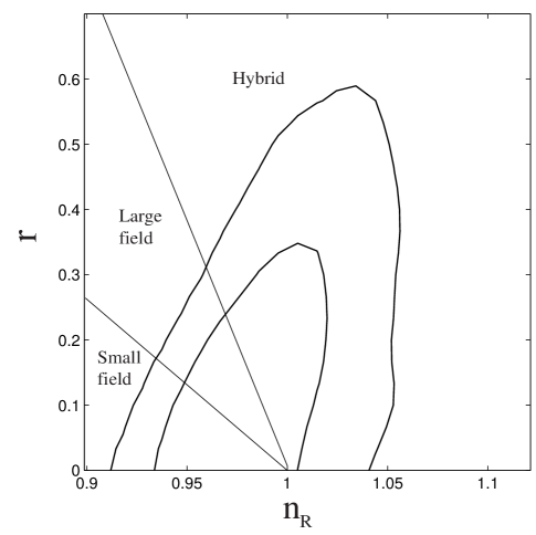
Figure 4: Classification of inflationary models in the $n_{\cal R}$-$r$ plane in the low-energy limit. The line $r=(8/3)(1-n_{\cal R})$ marks the border of large-field and small-field models, whereas the border of large-field and hybrid models corresponds to $r=8(1-n_{\cal R})$.

While there is no signature in CMB data of statistically significant deviations from the predictions of the single-field inflationary paradigm, the suppressed quadrupole WMAP is rather unexpected. Although the lack of power on the largest scales may be purely due to cosmic variance and hence statistically insignificant Efs03 , theoretically motivated explanations are not ruled out; see, e.g. Refs. Yokoyama99 ; Tsujiloop ; Tsuji03noncom ; Piao03 ; Piao04 ; Contaldi03 ; Feng03 ; Kawasaki03 ; BFM03 ; LMMR04 ; AS03 ; SP05 for a number of attempts to explain this loss of power on the largest scales.

V.2 Classification of inflation models in the $n_{\cal R}$-$r$ plane

By Eqs. (119) and (133) the general relation between $n_{\cal R}$ and $r$ is

$$r=\frac{8}{3}(1-n_{\cal R})+\frac{16}{3}\eta\,.$$ (139)

The border of large-field and small-field models is given by the linear potential

$$V=V_{0}\phi\,.$$ (140)

Since $V_{\phi\phi}$ vanishes in this case (i.e., $\eta=0$), we have $n_{\cal R}-1=-6\epsilon$ and

$$r=\frac{8}{3}(1-n_{\cal R})\,.$$ (141)

The exponential potential LM85 ; Yokoyama88

$$V=V_{0}\exp\left(-\sqrt{\frac{16\pi}{\alpha}}\frac{\phi}{m_{{\rm pl}}}\right)\,,$$ (142)

characterizes the $n\to\infty$ limit of the large field models in Eq.(25) and hence the border between large-field and hybrid models. In this case we have $\eta=2\epsilon=2/\alpha$ and

$$r=8(1-n_{\cal R})\,.$$ (143)

Then we can classify inflationary models such as (A) large-field ($0<\eta\leq 2\epsilon)$, (B) small-field ($\eta<0$), and (C) hybrid models ($\eta>2\epsilon$). This is illustrated in Fig. 4. The allowed range of hybrid models is wide relative to large-field and small-field models. We note that double inflation models are not categorised in above classes, since the discussion of density perturbations in the single-field case is not valid. We shall discuss this case separately in a later section.

The large-field potential (25) involves only one free parameter, $V_{0}$, for a given value of $n$. The small-field potential (28) has two parameters $V_{0}$ and $\mu$. The hybrid model involves more free parameters, e.g., $g,\lambda,M,m$ (4 parameters) for the potential (32). This implies that the small-field and hybrid models are difficult to be constrained relative to the large-field models, since these have additional freedom to be compatible with observational data. In fact the large-field models are severely constrained from current observations Barger03 ; Kinney04 ; Leach03 ; WMAP , while it is not so for small-field and hybrid models due to additional model parameters. In the next subsection we shall discuss the observational constraint on large-field models.

V.3 Observational constraints on large-field inflation

Let us consider the monomial potential (25). In this case the number of e-foldings is given as $N=4\pi/(nm_{\rm pl}^{2})(\phi^{2}-\phi_{f}^{2})$ with $\phi_{f}=nm_{\rm pl}/4\sqrt{\pi}$ being the value of inflaton at the end of inflation. Then the spectral index $n_{\cal R}$ and the tensor to scalar ratio $r$ are written in terms of the function of $N$:

$$n_{\cal R}=1-\frac{2(n+2)}{4N+1}\,,~{}~{}~{}r=\frac{16n}{4N+1}\,.$$ (144)

Note that these are independent of the energy scale $V_{0}$. In Fig. 5 we plot the theoretical values (144) for the quadratic ($n=2$) and the quartic ($n=4$) potentials with several different values of $N$. The predicted points for the quadratic potential are within the $1\sigma$ observational contour bound for the e-foldings greater than $N=45$, thus preferable observationally. The quartic potential is outside of the $2\sigma$ contour bound for the e-foldings less than $N=60$. Therefore the $n=4$ case is under strong observational pressure even with first year WMAP data unless the number of e-foldings is sufficiently large ($N>60$). This situation is improved if the inflaton is coupled to gravity with a negative non-minimal coupling KF99 ; TsujiBu .

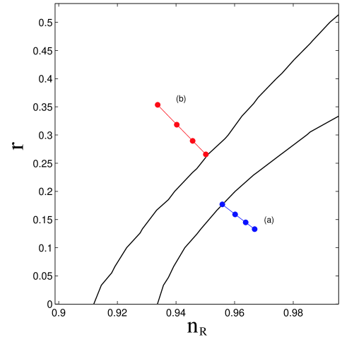
Figure 5: Theoretical prediction of large-field models together with the $1\sigma$ and $2\sigma$ observational contour bounds from first year WMAP data. Each case corresponds to (a) $n=2$ and (b) $n=4$ with e-foldings $N=45,50,55,60$ (from top to bottom) showing how models with few e-foldings are under severe pressure from observations.

The small-field and hybrid models involve more than two parameters, so we have a freedom to fit the model parameters so that it matches with the observational constraints. In this sense we can not currently rule out these models, although some of the model parameters can be constrained.

VI Perturbations generated in higher-dimensional models

There has been a lot of interest in the construction of early universe scenarios in higher-dimensional models motivated by string/M-theory. A well-known example is the Randall-Sundrum (RS) braneworld scenario RSI ; RSII , in which our four-dimensional brane is embedded in a five-dimensional bulk spacetime (see Ref. Maa03 ; BVD for reviews). In this scenario standard model particles are confined on the brane, while gravitons propagate in the bulk spacetime. Since the effect of the extra dimension induces additional terms at high energies, e.g., a quadratic term of energy density BDL ; SMS , this can lead to a larger amount of inflation relative to standard inflationary scenarios Maa99 ; Cope01 .

In conventional Kaluza-Klein theories, extra dimensions are compactified on some internal manifold in order to obtain a four-dimensional effective gravity. A simple cosmological model using toroidal compactifications is the Pre-Big-Bang (PBB) scenario Vene91 ; Gas93 , which is based upon the low-energy, tree-level string effective action (see also Refs. LWCreview ; Gas02 ). In this scenario there exist two branches–one of which is a dilaton-driven super inflationary stage and another is the Friedmann branch with a decreasing curvature. It is possible to connect the two branches by taking into account string loop and derivative corrections to the tree-level action Bru97 ; Foffa99 ; Cartier99 . If we transform the string-frame action to the four-dimensional Einstein frame, the universe exhibits a contraction with $a\propto(-t)^{1/3}$ in the PBB phase. Therefore the Pre-Big-Bang (PBB) scenario can be viewed as a bouncing cosmological model in the Einstein frame.

The ekpyrotic Khoury01 and cyclic Stein02 models have a similarity to the PBB scenario in the sense that the universe contracts before a bounce. In ekpyrotic/cyclic scenarios the collision of two parallel branes embedded in an extra-dimensional bulk signals the beginning of the hot, expanding, big bang of standard cosmology.

Models with a cosmological bounce potentially provide an alternative to inflation in addressing the homogeneity problem of big-bang cosmology and in yielding a causal mechanism of structure formation. In this sense it is important to evaluate the spectra of density perturbations in order to make contact with observations and distinguish these models from the inflationary scenario.

More recently there has been a lot of effort to construct more conventional inflationary models in string theory using D-branes (and anti D-branes) with a flux compactification in a warped geometry to give rise to de Sitter solutions in four-dimensions. We do not have enough space to review this emerging field, but refer readers to the other papers Dvali99 ; Quevedo02 ; Kachru03 ; Bur04 ; Blanco04 ; Garousi04 ; KSW05 . In principle we can evaluate the spectra of perturbations using the method in the previous sections once the effective potential of the inflaton is known in an effective 4-dimensional theory in four-dimensional gravity.

In the rest of this section we shall review brane-world, PBB and ekpyrotic/cyclic models in separate subsections.

VI.1 Braneworld

In the RSII model RSII the Einstein equations on our 3-brane can written as SMS :

$${}^{(4)}G_{\mu\nu}=-\Lambda_{4}g_{\mu\nu}+\frac{8\pi}{m_{{\rm pl}}^{2}}T_{\mu\nu}+\left(\frac{8\pi}{M_{5}^{3}}\right)^{2}\pi_{\mu\nu}-E_{\mu\nu}\,,$$ (145)

where $T_{\mu\nu}$ and $\pi_{\mu\nu}$ represent the energy–momentum tensor on the brane and a term quadratic in $T_{\mu\nu}$, respectively. $E_{\mu\nu}$ is a projection of the 5-dimensional Weyl tensor, which carries information about the bulk gravity. The 4- and 5-dimensional Planck masses, $m_{{\rm pl}}$ and $M_{5}$, are related via the 3-brane tension, $\lambda$, as

$$\lambda=\frac{3}{4\pi}\frac{M_{5}^{6}}{m_{{\rm pl}}^{2}}\,.$$ (146)

In what follows the 4-dimensional cosmological constant $\Lambda_{4}$ is assumed to be zero.

The Friedmann equation in the flat FRW background becomes

$$H^{2}\equiv\left(\frac{\dot{a}}{a}\right)^{2}=\frac{8\pi}{3m_{{\rm pl}}^{2}}\rho\left(1+\frac{\rho}{2\lambda}\right)\,,$$ (147)

where $\rho$ is the energy density of the matter on the brane. At high energies the $\rho^{2}$ term can play an important role in determining the evolution of the Universe. We neglected the contribution of the so-called “dark radiation”, $E_{\mu\nu}$, which decreases as $\sim a^{-4}$ during inflation. However we caution that this may be important in considering perturbations at later stages of cosmological evolution Koyama03 ; Rho03 .

The inflaton field $\phi$, confined to the brane, satisfies the 4D Klein–Gordon equation given in Eq. (19). The quadratic contribution in Eq. (147) increases the Hubble expansion rate during inflation, which makes the evolution of the inflaton slower than in the case of standard General Relativity. Combining Eq. (19) with Eq. (147), we obtain Maa99 ; TMM01

$$\frac{\ddot{a}}{a}=\frac{8\pi}{3m_{{\rm pl}}^{2}}\left[(V-\dot{\phi}^{2})+\frac{\dot{\phi}^{2}+2V}{8\lambda}(2V-5\dot{\phi}^{2})\right]\,.$$ (148)

The condition for inflation is $\ddot{a}>0$, which reduces to the standard expression $V>\dot{\phi}^{2}$ for $(\dot{\phi}^{2}+2V)/8\lambda\ll 1$. In the high-energy limit, this condition corresponds to $V>(5/2)\dot{\phi}^{2}$.

It was shown in Ref. Wands00 that the conservation of the curvature perturbation, ${\cal R}$, holds for adiabatic perturbations irrespective of the form of gravitational equations by considering the local conservation of the energy-momentum tensor. One has $|{\cal R}|\simeq(H/\dot{\phi})\delta\phi\simeq(H/\dot{\phi})(H/2\pi)$ after the Hubble-radius crossing, as in the case of standard General Relativity discussed in Sec. IV. Then we get the amplitude of scalar perturbations, as Maa99

$${\cal P}_{\cal R}\simeq\frac{H^{2}}{\dot{\phi}^{2}}\left(\frac{H}{2\pi}\right)^{2}\simeq\frac{128\pi}{3m_{{\rm pl}}^{6}}\,\frac{V^{3}}{V_{\phi}^{2}}\,\left(1+\frac{V}{2\lambda}\right)^{3}\,,$$ (149)

which is evaluated at the Hubble radius crossing, $k=aH$. Note that it is the modification of the Friedmann equation that changes the form of ${\cal P}_{\cal R}$ when it is expressed in terms of the potential.

Tensor perturbations in cosmology are more involved since gravitons propagate in the bulk. The equation for gravitational waves in the bulk corresponds to a partial differential equation with a moving boundary, which is not generally separable. However when the evolution on the brane is de Sitter, it is possible to make quantitative predictions about the evolution of gravitational waves in slow-roll inflation. The amplitude of tensor perturbations was evaluated in Ref. LMW00 , as

$${\cal P}_{\rm T}=\frac{64\pi}{m_{\rm Pl}^{2}}\left(\frac{H}{2\pi}\right)^{2}F^{2}(x)\,,$$ (150)

where $x=Hm_{{\rm pl}}\sqrt{3/(4\pi\lambda)}$ and

$$F(x)=\left[\sqrt{1+x^{2}}-x^{2}\sinh^{-1}(1/x)\right]^{-1/2}\,.$$ (151)

Here the function $F(x)$ appeared from the normalization of a zero-mode.

The spectral indices of scalar and tensor perturbations are

$$n_{{\cal R}}-1=-6\epsilon+2\eta\,,~{}~{}~{}n_{{\rm T}}=-\frac{2}{N_{\phi}}\frac{x_{\phi}}{x}\frac{F^{2}}{\sqrt{1+x^{2}}}\,,$$ (152)

where the modified slow-roll parameters are defined by

$$\epsilon \equiv \frac{m_{{\rm pl}}^{2}}{16\pi}\,\left(\frac{V_{\phi}}{V}\right)^{2}\;\frac{1+V/\lambda}{\left(1+V/2\lambda\right)^{2}}\,,$$ (153)

$$\eta \equiv \frac{m_{{\rm pl}}^{2}}{8\pi}\,\frac{V_{\phi\phi}}{V}\;\frac{1}{1+V/2\lambda}\,,$$ (154)

together with the number of e-foldings

$$N\simeq-\frac{8\pi}{m_{{\rm pl}}^{2}}\int^{\phi_{f}}_{\phi}\frac{V}{V_{\phi}}\left(1+\frac{V}{2\lambda}\right){\rm d}\phi\,.$$ (155)

By Eqs. (149), (150) and (152), one can show that the same consistency relation Eq. (134) relates the tensor-scalar ratio to the tilt of the gravitational wave spectrum, independently of the brane tension $\lambda$ Huey01 (see also Refs. Cal03 ; Cal03v2 ; Ramirez03 ). This degeneracy of the consistency relation means that to lowest order in slow-roll parameters it is not possible to observationally distinguish perturbations spectrum produced by braneworld inflation models from those produced by 4D inflation with a modified potential LiddleTaylor . If one uses horizon-flow parameters defined in Eq. (135), we obtain in the high-energy ($V\gg\lambda$) limit Tsuji04 ; Calshinji

$$n_{{\cal R}} = 1-3\epsilon_{1}-\epsilon_{2},~{}n_{{\rm T}}=-3\epsilon_{1},~{}r=24\epsilon_{1}\,,$$

$$\alpha_{{\cal R}} = -3\epsilon_{1}\epsilon_{2}-\epsilon_{2}\epsilon_{3}\,,~{}\alpha_{\rm T}=-3\epsilon_{1}\epsilon_{2}\quad({\rm for}~{}~{}V/\lambda\gg 1)\,.$$

We note that these results are identical to those given for 4D general relativity in Eq. (137) if one replaces $2\epsilon_{1}$ in Eq. (137) with $3\epsilon_{1}$ in Eq. (VI.1).

This correspondence suggests that a separate likelihood analysis of observational data is not needed for the braneworld scenario, as observations can be used to constrain the same parameterisation of the spectra produced. Therefore the observational contour bounds in Fig. 4 can be used in braneworld as well. However, when those constraints are then interpreted in terms of the form of the inflationary potential, differences can be seen depending on the regime we are in. In what follows we will obtain observational constraints on large-field potentials (25) under the assumption that we are in the high-energy regime ($\rho\gg\lambda$).

One can estimate the field value at the end of inflation by setting $\epsilon(\phi_{f})=1$. Then by Eqs. (VI.1) and (155), we get

$$n_{{\cal R}}-1 = -\frac{2(2n+1)}{N(n+2)+n}\,,$$ (157)

$$r = \frac{24n}{N(n+2)+n}\,.$$ (158)

Since $N(n+2)\gg n$ for the e-folds $N>50$, one can neglect the second term as in Ref. Tsuji04 . For a fixed value of $n$, $n_{\cal R}$ and $r$ are only dependent on $N$.

The quadratic potential ($n=2$) is within the $2\sigma$ observational contour bound for $N>50$ as found from Fig. 6. The quartic potential is outside the $2\sigma$ bound for $N<60$, which means that this model is under strong observational pressure. Note that the theoretical points tend to be away from the point $n_{\cal R}=1$ and $r=0$ compared to the standard General Relativistic inflation. Exponential potentials correspond to the limit $n\to\infty$, in which case we have $n_{\cal R}-1=-4/N$ and $r=24/N$ from Eqs. (157) and (158). This case does not lie within the $2\sigma$ bound unless $N>90$. Therefore steep inflation Cope01 driven by an exponential potential is excluded observationally Liddle03 ; Tsuji04 , unless other effects coming from a higher-dimensional bulk modifies the spectra of perturbations.

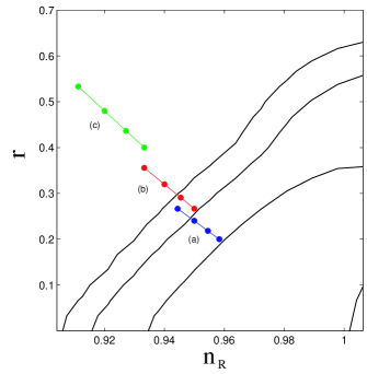
Figure 6: Constraints on large-field models in the context of braneworld Tsuji04 . We show theoretical predictions together with the $1\sigma$, $2\sigma$ and $3\sigma$ observational contour bounds. Each case corresponds to (a) $n=2$, (b) $n=4$ and (c) $n\to\infty$ (exponential potentials), respectively, with e-foldings $N=45,50,55,60$ (from top to bottom).

This situation changes if we consider the Gauss-Bonnet (GB) curvature invariant Lidsey03 in five dimensional gravity, arising from leading-order quantum corrections of the low-energy heterotic gravitational action TSM04 . One effect of the GB term is to break the degeneracy of the standard consistency relation DLMS04 . Although this does not lead to a significant change for the likelihood results of inflationary observables, the quartic potential is rescued from marginal rejection for a wide range of energy scales TSM04 .

Even steep inflation exhibits marginal compatibility for a sufficient number of e-foldings. This property is illustrated in Fig. 7. In Gauss-Bonnet (GB) braneworld the background equation is given as $H^{2}\propto\rho^{2/3}$ in a high-energy regime, whereas the RS regime is characterised by $H^{2}\propto\rho^{2}$. In both regions, the ratio $r$ is larger than in the case of General Relativity ($H^{2}\propto\rho$). The tensor to scalar ratio $r$ has a minimum in the intermediate energy region between the Gauss-Bonnet (extreme right) and Randall-Sundrum (extreme left) regimes TSM04 . As seen in Fig. 7 exponential potentials tend to enter the $2\sigma$ contour bound for $N>55$, thus showing the observational compatibility. (see Refs. DLMS04 ; TSM04 for more details).

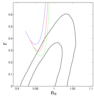
Figure 7: Observational constraints on exponential potentials in a Gauss-Bonnet braneworld for the e-foldings $N=50,60,70$ (from top to bottom). The theoretical curves are inside the $2\sigma$ contour bound for the e-folds $N>55$.

Finally we note that braneworld effects on the evolution of perturbations after the second Hubble radius crossing can potentially leave signatures on the temperature anisotropies in CMB, but the techniques for calculating these signatures are still under development Koyama03 ; Rho03 . While it is generally complicated to fully solve the perturbation equations in a higher-dimensional bulk coupled to matter perturbations on the brane Kodama00 ; Koyama00 ; vande00 ; BMW ; KMW05 ; Mukoh00 , it is of great interest to see how the effect of five-dimensional gravity affects the CMB power spectra by solving the bulk geometry consistently.

VI.2 Pre-big-bang and ekpyrotic/cyclic cosmologies

The PBB scenario can be characterized in four-dimensions by an effective action in the string frame Vene91 ; Gas93 :

$${\cal S}_{S}\,=\,\int{\rm d}^{4}x\sqrt{-g}e^{-\phi}\left[\frac{1}{2}R+\frac{1}{2}(\nabla\phi)^{2}-V_{S}(\phi)\right]\,,$$ (159)

where $\phi$ is the dilaton field with potential $V_{S}(\phi)$. Note that we neglect here additional modulus fields corresponding to the size and shape of the internal space of extra dimensions. The potential for the dilaton vanishes in the perturbative string effective action. The dilaton evolves from a weakly coupled regime ($e^{\phi}\ll 1$) toward a strongly coupled region during which the Hubble parameter grows (superinflation). This PBB branch connects to a Friedmann one with a decreasing Hubble rate if the singularity can be avoided leading to a maximum value for the Hubble parameter.

If we make a conformal transformation

$$\hat{g}_{\mu\nu}=e^{-\phi}g_{\mu\nu}\,,$$ (160)

the action in the Einstein frame can be written as

$${\cal S}_{E}\,=\,\int{\rm d}^{4}x\sqrt{-\hat{g}}\left[\frac{1}{2}\hat{R}-\frac{1}{4}(\hat{\nabla}\phi)^{2}-V_{E}(\phi)\right]\,,$$ (161)

where $V_{E}(\phi)\equiv e^{\phi}V_{S}(\phi)$. Introducing a rescaled field $\varphi=\pm\phi/\sqrt{2}$, the action (161) reads

$${\cal S}_{E}\,=\,\int{\rm d}^{4}x\sqrt{-\hat{g}}\left[\frac{1}{2}\hat{R}-\frac{1}{2}(\hat{\nabla}\varphi)^{2}-V_{E}(\phi(\varphi))\right]\,.$$ (162)

Then the action (159) can be used to describe both the PBB model in the Einstein frame, as well as the ekpyrotic scenario Durrer02 .

In the original version of the ekpyrotic scenario Khoury01 , the Einstein frame is used where the coupling to the Ricci curvature is fixed, and the field $\phi$ describes the separation of a bulk brane from our four-dimensional orbifold fixed plane. In the case of the second version of the ekpyrotic scenario Khoury02 and in the cyclic scenario Stein02 , $\phi$ is the modulus field denoting the size of the orbifold (the separation of the two orbifold fixed planes).

The ekpyrotic scenario is characterized by a negative exponential potential Khoury01

$$V_{E}=-V_{0}\exp\left(-\sqrt{\frac{2}{p}}\,\varphi\right)\,,$$ (163)

with $0<p\ll 1$. The branes are initially widely separated but are approaching each other, which means that $\varphi$ begins near $+\infty$ and is decreasing toward $\varphi=0$. The universe exhibits a contraction in this phase in the Einstein frame. In the PBB scenario the dilaton starts out from a weakly coupled regime with $\phi$ increasing from $-\infty$. If we want the potential (163) to describe a modified PBB scenario with a dilaton potential which is important when $\phi\to 0$ but negligible for $\phi\to-\infty$, we have to use the relation $\varphi=-\phi/\sqrt{2}$ between the field $\varphi$ in the ekpyrotic case and the dilaton $\phi$ in the PBB case.

In the flat FRW background the system with the exponential potential (163) has the following exact solution LM85 ; Lyth02ekp1 ; Durrer02 ; TBF02 ; Hwang02eky ; Tsujiekp ; HW02

$$a_{E}\propto|t_{E}|^{p},~{}H_{E}=\frac{p}{t_{E}},~{}V_{E}=-\frac{p(1-3p)}{t_{E}^{2}},~{}\dot{\varphi}=\frac{\sqrt{2p}}{t_{E}}\,,$$ (164)

where $p>0$ and the subscript “E ” denotes the quantities in the Einstein frame. The solution for $t_{E}<0$ describes the contracting universe prior to the collision of branes. Note that the PBB scenario corresponds to $p=1/3$, in which case the potential of the dilaton is absent. The ekpyrotic scenario corresponds to a slow contraction with $0<p\ll 1$. In the string frame we have Durrer02 ; TBF02

$$a_{S}\propto(-t_{S})^{-\sqrt{p}},~{}~{}~{}\phi=-\frac{2\sqrt{p}}{1-\sqrt{p}}\ln\left[-(1-\sqrt{p})t_{S}\right]\,.$$ (165)

This illustrates the super-inflationary solution with growing dilaton.

Let us evaluate the spectrum of scalar perturbations generated in the contracting phase given by Eq. (164). In this case we have $\epsilon=1/p$ and $\nu_{\cal R}^{2}=[(3p-1)/(1-p)]^{2}$ in Eq. (107). Then by using Eq. (118) we obtain the spectral index of curvature perturbations Wands98 ; Lyth02ekp1 (see also Refs. Lyth02ekp2 ; Bran01 ; Hwang02eky ; Tsujiekp ; TBF02 ; Allen04 ; Finelli02a ):

$$n_{\cal{R}}-1 = \frac{2}{1-p}~{}~{}~{}({\rm for}~{}~{}0<p\leq 1/3)\,,$$ (166)

$$= \frac{4-6p}{1-p}~{}~{}~{}({\rm for}~{}~{}1/3\leq p<1)\,.$$ (167)

We can obtain the above exact result of the perturbation spectra for exponential potentials without using slow-roll approximations. We see that a scale-invariant spectrum with $n_{\cal R}=1$ is obtained either as $p\to\infty$ in an expanding universe, corresponding to conventional slow-roll inflation, or for $p=2/3$ during collapse Star79 ; Wands98 . In the case of the PBB cosmology ($p=1/3$) one has $n_{\cal{R}}=4$, which is a highly blue-tilted spectrum. The ekpyrotic scenario corresponds to a slow contraction ($0<p\ll 1$), in which case we have $n_{\cal{R}}\simeq 3$.

The spectrum (167) corresponds to the one generated before the bounce. In order to obtain the final power spectrum at sufficient late-times in an expanding branch, we need to connect the contracting branch with the Friedmann (expanding) one. In the context of PBB cosmology, it was realized in Ref. Gas96 ; Bru97 (see also Rey96 ; Foffa99 ; Cartier99 ) that loop and higher derivative corrections (defined in the string frame) to the action induced by inverse string tension and coupling constant corrections can yield a nonsingular background cosmology. This then allows the study of the evolution of cosmological perturbations without having to use matching prescriptions. The effects of the higher derivative terms in the action on the evolution of fluctuations in the PBB cosmology was investigated numerically in Cartier01 ; TBF02 . It was found that the final spectrum of fluctuations is highly blue-tilted ($n_{\cal R}\simeq 4$) and the result obtained is the same as what follows from the analysis using matching conditions between two Einstein Universes Bru94 ; Der95 joined along a constant scalar field hypersurface.

In the context of ekpyrotic scenario nonsingular cosmological solutions were constructed in Ref. TBF02 by implementing higher-order loop and derivative corrections analogous to the PBB case. A possible set of corrections include terms of the form Gas96 ; Bru97 ; TBF02

$${\cal L}_{c}=-\frac{1}{2}\alpha^{\prime}\lambda\xi(\phi)\left[cR_{\rm GB}^{2}+d(\nabla\phi)^{4}\right]\,,$$ (168)

where $\xi(\phi)$ is a general function of $\phi$ and $R_{\rm GB}^{2}=R^{2}-4R^{\mu\nu}R_{\mu\nu}+R^{\mu\nu\alpha\beta}R_{\mu\nu\alpha\beta}$ is the Gauss-Bonnet term. The corrections ${\cal L}_{c}$ are the sum of the tree-level $\alpha^{\prime}$ corrections and the quantum $n$-loop corrections ($n=1,2,3,\cdots$), with the function $\xi(\phi)$ given by

$$\xi(\phi)=-\sum_{n=0}C_{n}e^{(n-1)\phi}\,,$$ (169)

where $C_{n}$ ($n\geq 1$) are coefficients of $n$-loop corrections, with $C_{0}=1$. Nonsingular bouncing solutions that connect to a Friedmann branch can be obtained by accounting for the corrections up to two-loop with a negative coefficient ($C_{2}<0$). See Ref. TBF02 for a detailed analysis on the background evolution.

It was shown in Ref. TBF02 that the spectrum of curvature perturbations long after the bounce is given as $n_{\cal R}\simeq 3$ for $0<p\ll 1$ by numerically solving perturbation equations in a nonsingular background regularized by the correction term (168). In particular comoving curvature perturbations are conserved on cosmologically relevant scales much larger than the Hubble radius around the bounce, which means that the spectrum (166) can be used in an expanding background long after the bounce.

The authors in KOST02 showed that the spectrum of the gravitational potential $\Phi$, defined in Eq. (45), generated before the bounce is nearly scale-invariant for $0<p\ll 1$, i.e., $n_{\Phi}-1=-2p/(1-p)$. A number of authors argued Lyth02ekp1 ; Lyth02ekp2 ; Bran01 ; Hwang02eky ; Hwang02eky2 that this corresponds to the growing mode in the contracting phase but to the decaying mode in the expanding phase. The authors in Ref. Cartier03 studied several toy bouncing models assuming non-singular second-order evolution equations for the perturbations across the bounce. They found that the final power spectrum is dependent on the details of the bounce model. However Cartier Cartier04 recently performed detailed numerical analysis using nonsingular perturbation equations and found that in the case of the $\alpha^{\prime}$-regularised bounce both $\Phi$ and ${\cal R}$ exhibit the highly blue-tilted spectrum (166) long after the bounce. It was numerically shown that the dominant mode of the gravitational potential is fully converted into the post-bounce decaying mode. Similar conclusions have also been reached in investigations of perturbations in other specific non-singular models Gasperini03 ; Gasperini04 ; Allen04 ; BG05 ; Bozza05 . Arguments can given that the comoving curvature perturbation is conserved for adiabatic perturbations on large scales under very general conditions Lyth03p1 ; CNZ05 .

Nevertheless we have to caution that these studies are based on non-singular four-dimensional bounce models and in the ekpyrotic/cyclic model the bounce is only non-singular in a higher-dimensional completion of the model Tolley02 . The ability of the ekpyrotic/cyclic model to produce a scale-invariant spectrum of curvature perturbations after the bounce relies on this higher-dimensional physics being fundamentally different from conventional four-dimensional physics, such that the growing mode of $\Phi$ in the contracting phase does not decay after the bounce Tolley03 .

The main reason we obtain the blue-tilted spectrum for curvature perturbations in a contracting universe is that the system is characterised by a kinematic driven phase not by a slow-roll phase. In the case of modulus-driven superinflation with a Gauss-Bonnet term, the spectrum of scalar perturbations is $n_{\cal R}=10/3$ Kawai99 ; Tsujiekp , which is again highly blue-tilted. This is contrast with slow-roll inflation in which nearly scale-invariant spectra are automatically obtained when the slow-roll conditions ($\epsilon\ll 1,|\eta|\ll 1$) are satisfied. Therefore slow-roll inflation is typically more “stable” than kinematic-driven scalar field models to generate scale-invariant spectra in a generic way.

This perturbation spectra can be changed by taking into account a second scalar field Bozza02 ; Notari02 ; DiMarco03 . A system with multiple scalar fields generally induces isocurvature perturbations, which can be the source of adiabatic perturbations as we will discuss in Section VII. For instance, axion fields can acquire scale-invariant perturbation spectra due to their non-minimal coupling to the dilaton field in the PBB Copeland77 ; Sta01 ; DiMarco03 . Although these isocurvature perturbations are decoupled from curvature perturbation during the PBB collapse phase they could in principle provide a source for curvature perturbations at the bounce LLKCreview , or through the decay of massive axions during the expanding phase Enqvist02 ; Lyth02 , in an application of the curvaton idea which we will discuss in Section XII. The authors of ref. Notari02 considered a specific two-field system with a brane-modulus $\varphi$ and a dilaton $\chi$. When the dilaton has a negative exponential potential with a suppressed ekpyrotic potential for $\varphi$, the entropy “field” perturbation can be scale-invariant if the model parameters are fine-tuned Notari02 . It is certainly possible to construct non-singular multi-field PBB/ekpyrotic/cyclic scenarios that provide flat power spectra at late times independent of arguments over gauge choices for metric perturbations.

VII Adiabatic and entropy perturbations from inflation

Realistic inflationary models, embedded in GUT or supersymmetric theories, must necessarily be theories of multiple fields and it is fairly natural to have multiple phase of inflation (e.g. ARS97 ; julien ; subir ; chain ; Kadota03 ). In such models with more than one scalar field we have to consider the effect upon the evolution of non-adiabatic fluctuations in any light fields whose effective mass is less than the Hubble scale.

In the presence of more than one light field the vacuum fluctuations stretched to super-Hubble scales will inevitably include isocurvature modes during inflation. It is important to emphasise that this does not mean that the “primordial” density perturbation (at the epoch of primordial nucleosynthesis) will contain isocurvature modes. In particular, if the universe undergoes conventional reheating phase at the end of inflation and all particle species are in thermal equilibrium with their abundances determined by a single temperature (with no non-zero chemical potentials) then the primordial perturbations must be adiabatic Weinberg04b . It is these primordial perturbations that set the initial conditions for the evolution of radiation-matter fluid that determines the anisotropies in the cosmic microwave background and large-scale structure in our Universe and thus are directly constrained by observations. We will see that while the existence of non-adiabatic perturbations after inflation requires the existence of non-adiabatic perturbations during inflation Weinberg04a , it is not true that isocurvature modes during inflation necessarily give primordial isocurvature modes Weinberg04b .

VII.1 Inflaton and entropy perturbations during inflation

Following Gordon00 (see also Groot01 ; Rigopoulos ) we will identify the inflaton as the direction in field space corresponding to the evolution of the background (homogeneous) field. Thus for $n$ scalar fields $\varphi_{I}$, where $I$ runs from $1$ to $n$, we have

$$\sigma=\int\sum_{I}\hat{\sigma}_{I}\dot{\varphi}_{I}{\rm d}t\,,$$ (170)

where the inflaton direction is defined by

$$\hat{\sigma}_{I}\equiv\frac{\dot{\varphi}_{I}}{\sqrt{\sum_{J}\dot{\varphi}_{J}^{2}}}\,.$$ (171)

Arbitrary field perturbations can be decomposed into adiabatic perturbations along the inflaton trajectory and $n-1$ entropy perturbations orthogonal to the inflaton in field space:

$$\delta\sigma = \sum_{I}\hat{\sigma}_{I}\delta\varphi_{I}\,,$$ (172)

$$\delta s_{I} = \sum_{J}\hat{s}_{IJ}\delta\varphi_{J}\,,$$ (173)

where $\sum_{I}\hat{s}_{JI}\hat{\sigma}_{I}=0$. Without loss of generality we assume that the entropy fields are also mutually orthogonal in field space. Note that we have assumed that the fields have canonical kinetic terms, that is, the field space metric is flat. See Refs. Groot01 ; DiMarco03 for the generalisation to non-canonical kinetic terms.

The $n$ evolution equations for the homogeneous scalar fields (III.2.1) can then be written as the evolution for a single inflaton field (19)

$$\ddot{\sigma}+3H\dot{\sigma}+V_{\sigma}=0\,,$$ (174)

where the potential gradient in the direction of the inflaton is

$$V_{\sigma}\equiv\frac{{\rm d}V}{{\rm d}\sigma}=\sum_{I}\hat{\sigma}_{I}V_{I}\,.$$ (175)

The total energy density and pressure are given by the usual single field result (17).

Similarly the total momentum and pressure perturbation (74) and (73) for $n$ scalar field perturbations can be written as for a single inflaton field

$$\delta q = -\dot{\sigma}\delta\sigma\,,$$ (176)

$$\delta P = \dot{\sigma}(\dot{\delta\sigma}-\dot{\sigma}A)-V_{\sigma}\delta\sigma\,.$$ (177)

However the density perturbation is given by

$$\delta\rho=\dot{\sigma}(\dot{\delta\sigma}-\dot{\sigma}A)+V_{\sigma}\delta\sigma+2\delta_{s}V\,,$$ (178)

where the deviation from the single field result (72) arises due to the perturbation of the potential orthogonal to the inflaton trajectory:

$$\delta_{s}V\equiv\sum_{I}V_{I}\delta\varphi_{I}-V_{\sigma}\delta\sigma\,.$$ (179)

The non-adiabatic pressure perturbation (49) is written as

$$\delta P_{\rm nad}=-\frac{2V_{\sigma}}{3H\dot{\sigma}}\delta\rho_{m}-2\delta_{s}V\,,$$ (180)

where the comoving density perturbation, $\delta\rho_{m}$, is given by Eq. (51). Although Eq. (63) requires the comoving density perturbation to become small on large scales, as in the single field case, there is now an additional contribution due to non-adiabatic perturbations of the potential which need not be small on large scales (This generalises the result of Ref. Gordon00 for two scalar fields to the case of $n$ canonical fields). We note that the dynamics of cosmological perturbations in multi-field system was investigated by a host of authors, see Refs. Bartolo01p1 ; Chiba97 ; Linde85 ; Salopek89 ; Sta94 ; Sta01 ; FRV04 ; Garcia95 ; Garcia96 ; HY05 ; Hwang00 ; Kadota03 ; Kadota03v2 ; Kana00p1 ; Kawasaki01 ; Polarski94 ; Sasaki95 ; Sasaki98 ; Langlois99 ; Langlois00 ; Mukhanov97 ; Kofman87 ; Kofman88 ; Lahiri .

VII.2 Evolution of non-adiabatic perturbations

We will now consider the coupled evolution of two canonical scalar fields, $\phi$ and $\chi$, during inflation and how this can give rise to correlated curvature and entropy perturbations. We will use the local rotation in field space defined by Eq. (172) and (173) to describe the instantaneous adiabatic and entropy field perturbations.

Note that the inflaton field perturbation (172) is gauge-dependent and thus we have to fix the gauge in order to obtain a gauge-invariant variable. We will choose to work with the inflaton perturbation in the spatially flat ($\psi=0$) gauge:

$$\delta\sigma_{\psi}\equiv\delta\sigma+\frac{\dot{\sigma}}{H}\psi\,.$$ (181)

By contrast the orthogonal entropy perturbation (173) is automatically gauge-invariant.

The generalisation to two fields of the evolution equation for the inflaton field perturbations in the spatially flat gauge, given in Eq. (102) for a single field, is Gordon00

$$\ddot{\delta\sigma}_{\psi}+3H\dot{\delta\sigma}_{\psi}+\left[\frac{k^{2}}{a^{2}}+V_{\sigma\sigma}-\dot{\theta}^{2}-\frac{8\pi G}{a^{3}}\frac{{\rm d}}{{\rm d}t}\left(\frac{a^{3}\dot{\sigma}^{2}}{H}\right)\right]\delta\sigma_{\psi}$$

$$=~{}~{}~{}2\frac{{\rm d}}{{\rm d}t}(\dot{\theta}\delta s)-2\left({V_{\sigma}\over\dot{\sigma}}+{\dot{H}\over H}\right)\dot{\theta}\delta s\,,$$ (182)

and the entropy perturbation obeys

$$\ddot{\delta s}+3H\dot{\delta s}+\left(\frac{k^{2}}{a^{2}}+V_{ss}+3\dot{\theta}^{2}\right)\delta s={\dot{\theta}\over\dot{\sigma}}{k^{2}\over 2\pi Ga^{2}}\Psi\,,$$ (183)

where $\tan\theta=\dot{\chi}/\dot{\phi}$ and

$$V_{\sigma\sigma} \equiv (\cos^{2}\theta)V_{\phi\phi}+(\sin 2\theta)V_{\phi\chi}+(\sin^{2}\theta)V_{\chi\chi},$$ (184)

$$V_{ss} \equiv (\sin^{2}\theta)V_{\phi\phi}-(\sin 2\theta)V_{\phi\chi}+(\cos^{2}\theta)V_{\chi\chi}.$$ (185)

We can identify a purely adiabatic mode where $\delta s=0$ on large scales. However a non-zero entropy perturbation does appear as a source term in the perturbed inflaton equation whenever the inflaton trajectory is curved in field space, i.e., $\dot{\theta}\neq 0$. We note that $\dot{\theta}$ is given by Gordon00

$$\dot{\theta}=-\frac{V_{s}}{\dot{\sigma}}\,,$$ (186)

where $V_{s}$ is the potential gradient orthogonal to the inflaton trajectory in field space.

The entropy perturbation evolves independently of the curvature perturbation on large-scales. It couples to the curvature perturbation only through the gradient of the longitudinal gauge metric potential, $\Psi$. Thus entropy perturbations are also described as “isocurvature” perturbations on large scales. Eq. (VII.2) shows that the entropy perturbation $\delta s$ works as a source term for the adiabatic perturbation. This is in fact clearly seen if we take the time derivative of the curvature perturbation Gordon00 :

$$\dot{\cal R}=\frac{H}{\dot{H}}\frac{k^{2}}{a^{2}}\Psi+\frac{2H}{\dot{\sigma}}\dot{\theta}\delta s\,.$$ (187)

Therefore ${\cal R}$ is not conserved even in the large-scale limit in the presence of the entropy perturbation $\delta s$ with a non-straight trajectory in field space ($\dot{\theta}\neq 0$).

Analogous to the single field case we can introduce slow-roll parameters for light, weakly coupled fields Wands02 . At first-order in a slow-roll expansion, the inflaton rolls directly down the potential slope, that is $V_{s}\simeq 0$. Thus we have only one slope parameter

$$\epsilon\equiv-\frac{\dot{H}}{H^{2}}\simeq\frac{1}{16\pi G}\left(\frac{V_{\sigma}}{V}\right)^{2}\,,$$ (188)

but three parameters, $\eta_{\sigma\sigma}$, $\eta_{\sigma s}$ and $\eta_{ss}$, describing the curvature of the potential, where

$$\eta_{IJ}\equiv\frac{1}{8\pi G}\frac{V_{IJ}}{V}\,.$$ (189)

The background slow-roll solution is described by

$$\dot{\sigma}^{2}\simeq\frac{2}{3}\epsilon V\,,\quad H^{-1}\dot{\theta}\simeq-\eta_{\sigma s}\,,$$ (190)

while the perturbations obey

$$H^{-1}\dot{\delta\sigma} \simeq \left(2\epsilon-\eta_{\sigma\sigma}\right)\delta\sigma-2\eta_{\sigma s}\delta s\,,$$

$$H^{-1}\dot{\delta s} \simeq -\eta_{ss}\delta s\,,$$ (191)

on large scales, where we neglect spatial gradients. Although $V_{s}\simeq 0$ at lowest order in slow-roll, this does not mean that the inflaton and entropy perturbations decouple. $\dot{\theta}$ given by Eq. (190) is in general non-zero at first-order and large-scale entropy perturbations do affect the evolution of the adiabatic perturbations when $\eta_{\sigma s}\neq 0$.

While the general solution to the two second-order perturbation equations (VII.2) and (183) has four independent modes, the two first-order slow-roll equations (VII.2) give the approximate form of the squeezed state on large scales. This has only two modes which we can describe in terms of dimensionless curvature and isocurvature perturbations:

$${\cal R}\equiv\frac{H}{\dot{\sigma}}\delta\sigma_{\psi}\,,\quad{\cal S}\equiv\frac{H}{\dot{\sigma}}\delta s\,.$$ (192)

The normalisation of ${\cal R}$ coincides with the standard definition of the comoving curvature perturbation, Eq. (53). The normalisation of the dimensionless entropy, ${\cal S}$, is chosen here coincide with Ref. Wands02 . It can be related to the non-adiabatic pressure perturbation (49) on large scales

$$\delta P_{\rm nad}\simeq-\epsilon\eta_{\sigma s}\frac{H^{2}}{2\pi G}{\cal S}\,.$$ (193)

The slow-roll approximation can provide a useful approximation to the instantaneous evolution of the fields and their perturbations on large scales during slow-roll inflation, but is not expected to remain accurate when integrated over many Hubble times, where inaccuracies can accumulate. In single-field inflation the constancy of the comoving curvature perturbation after Hubble exit, which does not rely on the slow-roll approximation, is crucial in order to make accurate predictions of the primordial perturbations using the slow-roll approximation only around Hubble crossing. In a two-field model we must describe the evolution after Hubble exit in terms of a general transfer matrix:

$$\left(\begin{array}[]{c}{{\cal R}}\\ {{\cal S}}\end{array}\right)=\left(\begin{array}[]{cc}1&{T}_{{\cal R}{\cal S}}\\ 0&{T}_{{\cal S}{\cal S}}\end{array}\right)\left(\begin{array}[]{c}{\cal R}\\ {\cal S}\end{array}\right)_{*}\,.$$ (194)

On large scales the comoving curvature perturbation still remains constant for the purely adiabatic mode, corresponding to ${\cal S}=0$, and adiabatic perturbations remain adiabatic. These general results are enough to fix two of the coefficients in the transfer matrix, but ${T}_{{\cal R}{\cal S}}$ and ${T}_{{\cal S}{\cal S}}$ remain to be determined either within a given theoretical model, or from observations, or ideally by both. The scale-dependence of the transfer functions depends upon the inflaton-entropy coupling at Hubble exit during inflation and can be given in terms of the slow-roll parameters as Wands02

$$\frac{\partial}{\partial\ln k}{T}_{{\cal R}{\cal S}} = 2\eta_{\sigma s}+(2\epsilon-\eta_{\sigma\sigma}+\eta_{ss}){T}_{{\cal R}{\cal S}}\,,$$

$$\frac{\partial}{\partial\ln k}{T}_{{\cal S}{\cal S}} = (2\epsilon-\eta_{\sigma\sigma}+\eta_{ss}){T}_{{\cal S}{\cal S}}\,.$$ (195)

VII.3 Initial power spectra

For weakly-coupled, light fields (with effective mass less than the Hubble scale) we can neglect interactions on wavelengths below the Hubble scale, so that vacuum fluctuations give rise to a spectrum of uncorrelated field fluctuations on the Hubble scale ($k=aH$) during inflation:

$${\cal P}_{\delta\varphi_{I}}\simeq\left(\frac{H}{2\pi}\right)_{*}^{2}\,,$$ (196)

where we use a $*$ to denote quantities evaluated at Hubble-exit. If a field has a mass comparable to the Hubble scale or larger then the vacuum fluctuations on wavelengths greater than the effective Compton wavelength are suppressed. In addition fluctuations in strongly interacting fields may develop correlations before Hubble exit. But in the slow-roll limit of weakly coupled, light fields the vacuum fluctuations in orthogonal fields are independent at Hubble-exit. This remains true under a local rotation in fields space to another orthogonal basis such as the instantaneous inflaton and entropy directions (172) and (173) in field space.

The curvature and isocurvature power spectra at Hubble-exit are given by

$$\left.{\cal P}_{{\cal R}}\right|_{*}\simeq\left.{\cal P}_{{\cal S}}\right|_{*}\simeq\left(\frac{H^{2}}{2\pi\dot{\sigma}}\right)_{*}^{2}\simeq\frac{8}{3}\left(\frac{V}{\epsilon M_{\rm Pl}^{4}}\right)_{*}\,,$$ (197)

while the cross-correlation is zero, at lowest order in slow-roll:

$$\left.{\cal C}_{{\cal R}{\cal S}}\right|_{*}\simeq 0\,.$$ (198)

The normalisation chosen for the dimensionless entropy perturbation in Eq. (192) ensures that the curvature and isocurvature fluctuations have the same power at horizon exit Wands02 . The spectral tilts at horizon-exit are also the same and are given by

$$n_{\cal R}|_{*}-1\simeq n_{\cal S}|_{*}\simeq-6\epsilon+2\eta_{\sigma\sigma}\,.$$ (199)

where $n_{\cal S}\equiv{\rm d}\ln{\cal P}_{\cal S}/{\rm d}\ln k$.

The tensor spectrum is decoupled from scalar metric perturbations at first-order and hence has the same form as in single field inflation, described in section IV. Thus the power spectrum of gravitational waves on super-Hubble scales during inflation is given by

$${\cal P}_{\rm T}\simeq\frac{16H^{2}}{\pi M_{\rm Pl}^{2}}\simeq\frac{128}{3}\frac{V_{*}}{M_{\rm Pl}^{4}}\,,$$ (200)

and the spectral tilt is

$$n_{\rm T}\simeq-2\epsilon\,.$$ (201)

VII.4 Primordial power spectra

The resulting primordial power spectra on large scales can be obtained simply by applying the general transfer matrix (194) to the initial scalar perturbations. There scalar power spectra probed by astronomical observations are thus given by Wands02

$${\cal P}_{\cal R} = (1+T_{{\cal R}{\cal S}}^{2}){\cal P}_{\cal R}|_{*}$$ (202)

$${\cal P}_{\cal S} = T_{{\cal S}{\cal S}}^{2}{\cal P}_{\cal R}|_{*}$$ (203)

$${\cal C}_{{\cal R}{\cal S}} = T_{{\cal R}{\cal S}}T_{{\cal S}{\cal S}}{\cal P}_{\cal R}|_{*}\,.$$ (204)

The cross-correlation can be given in terms of a dimensionless correlation angle:

$$\cos\Delta\equiv\frac{{\cal C}_{{\cal R}{\cal S}}}{\sqrt{{\cal P}_{\cal R}{\cal P}_{\cal S}}}=\frac{T_{{\cal R}{\cal S}}}{\sqrt{1+T_{{\cal R}{\cal S}}^{2}}}\,.$$ (205)

We see that if we can determine the dimensionless correlation angle, $\Delta$, from observations, then this determines the off-diagonal term in the transfer matrix

$$T_{{\cal R}{\cal S}}=\cot\Delta\,,$$ (206)

and we can in effect measure the contribution of the entropy perturbation during inflation to the resultant curvature perturbation. In particular this allows us in principle to deduce from observations the power spectrum of the curvature perturbation at Hubble-exit during inflation Wands02 :

$${\cal P}_{\cal R}|_{*}={\cal P}_{\cal R}\sin^{2}\Delta\,.$$ (207)

The scale-dependence of the resulting scalar power spectra depends both upon the scale-dependence of the initial power spectra and of the transfer coefficients. The spectral tilts are given from Eqs. (202–204) by

$$n_{\cal R} = n_{\cal R}|_{*}+H_{*}^{-1}(\partial{T}_{{\cal R}{\cal S}}/\partial t_{*})\sin 2\Delta\,,$$

$$n_{\cal S} = n_{\cal R}|_{*}+2H_{*}^{-1}(\partial\ln{T}_{{\cal S}{\cal S}}/\partial t_{*})\,,$$ (208)

$$n_{\cal C} = n_{\cal R}|_{*}+H_{*}^{-1}\left[(\partial{T}_{{\cal R}{\cal S}}/\partial t_{*})\tan\Delta+(\partial\ln{T}_{{\cal S}{\cal S}}/\partial t_{*})\right]\,,$$

where we have used Eq. (206) to eliminate $T_{{\cal R}{\cal S}}$ in favour of the observable correlation angle $\Delta$. Substituting Eq. (199) for the tilt at Hubble-exit, and Eqs. (VII.2) for the scale-dependence of the transfer functions, we obtain Wands02

$$n_{{\cal R}} \simeq 1-(6-4\cos^{2}\Delta)\epsilon$$

$$+2\left(\eta_{\sigma\sigma}\sin^{2}\Delta+2\eta_{\sigma s}\sin\Delta\cos\Delta+\eta_{ss}\cos^{2}\Delta\right)\,,$$

$$n_{\cal S} \simeq -2\epsilon+2\eta_{ss}\,,$$ (209)

$$n_{\cal C} \simeq -2\epsilon+2\eta_{ss}+2\eta_{\sigma s}\tan\Delta\,.$$

Although the overall amplitude of the transfer functions are dependent upon the evolution after Hubble-exit and through reheating into the radiation era, the spectral tilts can be expressed solely in terms of the slow-roll parameters at Hubble-exit during inflation and the correlation angle, $\Delta$, which can in principle be observed.

The gravitational wave power spectrum is frozen-in on large scales, independent of the scalar perturbations, and hence

$${\cal P}_{\rm T}|_{*}={\cal P}_{\rm T}\,.$$ (210)

Thus we can derive a modified consistency relation (134) between observables applicable in the case of two-field slow-roll inflation:

$$r=\frac{{\cal P}_{\rm T}}{{\cal P}_{\cal R}}\simeq-8n_{\rm T}\sin^{2}\Delta\,.$$ (211)

This relation was first obtained in Ref. Bartolo01p2 at the end of two-field inflation, and verified in Ref. Tsuji03 for slow-roll models. But it was realised in Ref. Wands02 that this relation also applies to the observable perturbation spectra some time after two-field slow-roll inflation has ended.

If there is another source of the scalar curvature perturbation, such as from a third scalar field during inflation, then this could give an additional contribution to the scalar curvature spectrum without affecting the gravitational waves, and hence the more general result becomes an inequality:

$$r\lesssim-8n_{\rm T}\sin^{2}\Delta\,.$$ (212)

VIII Correlations and the CMB

The physical processes that drive inflation in the early universe leave their mark in the perturbation spectra that are generated from vacuum fluctuations. Single field models yield only adiabatic perturbations on large scales during inflation, and adiabatic perturbations stay adiabatic on large scales. In multi-field models we have seen that perturbations orthogonal to the inflaton trajectory describe non-adiabatic perturbations, ${\cal S}_{*}$ in Eq. (194). These have two principal observational effects as shown in Eq. (194). Firstly they can alter the large scale curvature perturbation in the radiation era, through the off-diagonal term $T_{{\cal R}{\cal S}}$ in the transfer matrix. And secondly they can yield a primordial isocurvature perturbation, through $T_{{\cal S}{\cal S}}$. These relative perturbations between different components of the cosmic energy-momentum tensor yield distinctive observational features which enable the amplitude of such perturbations to be tightly constrained.

Up until 1999 all studies of the effect of isocurvature modes only considered isocurvature perturbations statistically independent of the primordial curvature perturbation, i.e., uncorrelated. But the off-diagonal term in the transfer matrix would give rise to correlations between primordial curvature and isocurvature modes, parameterised through the correlation angle, $\Delta$ in Eq. (206). Langlois Langlois99 pointed out that isocurvature perturbations produced during inflation might naturally be correlated with the adiabatic mode. Bucher et al Bucher99 pointed out that the most general primordial perturbations spectra could include several isocurvature modes (including neutrino density and velocity perturbations) and these would in general be correlated with the curvature perturbation and with one another Trotta01 .

The contribution of isocurvature perturbations to the overall CMB angular power spectrum is now tightly constrained due to the distinctive peak structure of adiabatic versus isocurvature modes. However in seeking observational signatures of isocurvature modes one must include the effect of correlations which introduces a different angular power spectrum. In effect one must include an additional term in the CMB angular power spectrum which, in contrast to the uncorrelated spectra, can be negative as well as positive (though the resulting angular power spectrum must remain non-negative). For instance this could actually decrease the angular power spectrum on large angular scales due to correlated isocurvature perturbations in some models of dark energy, as recently noted in Refs. MTde ; GordonHu .

VIII.1 Matter isocurvature modes

The most commonly considered isocurvature modes are perturbations in the density of non-relativistic matter (either baryons or cold dark matter) relative to the radiation energy density. This is given from Eq. (83) as

$${\cal S}_{m}=\frac{\delta\rho_{m}}{\rho_{m}}-\frac{3}{4}\frac{\delta\rho_{\gamma}}{\rho_{\gamma}}\,,$$ (213)

and hence in effect reduces to the fractional matter density perturbation deep in the primordial radiation dominated era when $\rho_{\gamma}\gg\rho_{m}$. On large scales both the primordial curvature perturbation, $\zeta_{\gamma}$, and the matter isocurvature perturbation, ${\cal S}_{m}$, are conserved on large scales Wands00 . In the rest of this section we shall adopt the notation of section VII and use ${\cal R}=-\zeta_{\gamma}$ on large scales to denote the primordial curvature perturbation.

After matter domination the matter perturbations come to dominate the total curvature perturbation, $\zeta$ given in Eq. (82), which we can write in terms of the primordial curvature and isocurvature perturbations as

$$\zeta_{m}=-{\cal R}+\frac{1}{3}{\cal S}_{m}\,,$$ (214)

where for simplicity we neglect the neutrino density. This is in turn related to the longitudinal gauge metric perturbation, Eq. (45), on large scales during the matter dominated era Mukhanov90

$$\Phi=\frac{3}{5}{\cal R}\,.$$ (215)

Temperature anisotropies in the CMB on large angular scales due to the intrinsic temperature perturbation plus the Sachs-Wolfe effect are given by Gordon02

$$\frac{\delta T}{T}\simeq\zeta_{\gamma}+2\Phi\,,$$ (216)

which can thus be written in terms of the primordial curvature and isocurvature perturbations using Eq. (214) as

$$\frac{\delta T}{T}\simeq\frac{1}{5}\left({\cal R}-2{\cal S}_{m}\right)\,.$$ (217)

Isocurvature matter perturbations also produce acoustic peaks but these are out of phase with those from adiabatic perturbations Bucher99 . The success of the minimal model based on scale-invariant, Gaussian and adiabatic perturbations in reproducing the detailed structure of acoustic peaks in the angular power spectrum means that models of structure formation based on isocurvature primordial perturbations are now convincingly ruled out. These models in any case required a steep blue spectrum of isocurvature perturbations in order to overcome the suppression of the contribution of isocurvature perturbations to the matter power spectrum on smaller scales Peacock . An almost scale-invariant spectrum of isocurvature perturbations, e.g., from fields obeying slow-roll conditions during inflation, gives a relatively small effect on the CMB on sub-Hubble scales at the time of last scattering Langlois00 ; Bucher99 ; Amendola02 .

There have been several different analyses of the observational constraints on isocurvature matter perturbations incorporating the first-year WMAP data and additional astronomical data on smaller scales Peiris03 ; Gordon02 ; Valiviita03 ; Crotty03 ; Parkinson04 ; Beltran04 ; Beltran05 ; Kurki-Suonio04 .

In a Bayesian analysis the posterior likelihood of quantities such as the amplitude of isocurvature modes relative to curvature perturbations inevitably depends both on the parameterisation chosen for the isocurvature modes and prior distribution chosen for those parameters. For the slow-roll two-field inflation described in section VII it is natural to adopt a power-law parameterisation for the perturbations at Hubble-exit:

$${\cal P}_{\cal R}|_{*}={\cal P}_{\cal S}|_{*}=A_{r}^{2}\left(\frac{k}{k_{0}}\right)^{n_{1}}\,,$$ (218)

and the transfer functions

$$T_{{\cal R}{\cal S}} = T_{r}\left(\frac{k}{k_{0}}\right)^{\Delta n_{r}/2}\,,$$ (219)

$$T_{{\cal S}{\cal S}} = T_{s}\left(\frac{k}{k_{0}}\right)^{\Delta n_{s}/2}\,.$$ (220)

This gives the primordial power spectra (202–204)

$${\cal P}_{\cal R} = A_{r}^{2}\left(\frac{k}{k_{0}}\right)^{n_{1}}+A_{s}^{2}\left(\frac{k}{k_{0}}\right)^{n_{3}}\,,$$ (221)

$${\cal P}_{\cal S} = B^{2}\left(\frac{k}{k_{0}}\right)^{n_{2}}\,,$$ (222)

$${\cal C}_{{\cal R}{\cal S}} = A_{s}B\left(\frac{k}{k_{0}}\right)^{n_{c}}\,,$$ (223)

where

$$A_{s}^{2}=T_{r}^{2}A_{r}^{2}\,,\quad n_{3}=n_{1}+\Delta n_{r}\,,$$ (224)

$$B^{2}=T_{s}^{2}A_{r}^{2}\,,\quad n_{2}=n_{1}+\Delta n_{s}\,,$$ (225)

and

$$n_{c}=\frac{n_{2}+n_{3}}{2}\,.$$ (226)

This coincides with the parameterisation used by Kurki-Suonio et al Kurki-Suonio04 , although they choose the opposite sign convention for the primordial curvature perturbation and hence the correlation angle. They find an upper limit (95% c.l.) on the allowed isocurvature fraction (marginalising over other parameters)

$$f_{\rm iso}\equiv\sqrt{\frac{B^{2}}{A_{r}^{2}+A_{s}^{2}}}<0.47\,,$$ (227)

where they use a pivot scale $k_{0}=0.01{\rm Mpc}^{-1}$. (Note that results in Kurki-Suonio04 are given in terms of $\alpha=f_{\rm iso}^{2}/(1+f_{\rm iso}^{2})$ for which they choose a flat prior.) By contrast an uncorrelated subset with $\cos\Delta\simeq 0$ yields a weaker limit of only $f_{\rm iso}<0.53$ as uncorrelated models have less effect on the CMB. The best-fit model of Ref. Kurki-Suonio04 has primordial power spectra with $n_{1}=-0.012$, $n_{2}=-0.074$, $n_{3}=-0.612$ and isocurvature fraction $f_{\rm iso}=0.044$ and correlation $\cos\Delta=0.82$. The principal effect of the correlated isocurvature perturbations (small at the pivot scale of $10$ Mpc) is to reduce the power in the lowest multipoles for these red primordial power spectra with $n_{\cal R}-1<0$. Use of a larger pivot scale $k_{0}$ in the analysis tends to favour these models Beltran04 . But in general isocurvature models are not favoured. Isocurvature modes do not produce the peak structure seen in the current data.

Note that the WMAP team Peiris03 restricted their analysis to a scale-invariant correlation which corresponds to $\Delta n_{r}=0$ above. They found $f_{\rm iso}<0.33$ at 95% c.l. using a pivot scale of $k_{0}=0.05{\rm Mpc}^{-1}$.

In Ref. Parkinson04 the double inflation model (32) was constrained by using the 1-st year WMAP data for the supersymmetric case ($g^{2}/\lambda=2$). It was found that the correlated isocurvature component can be at most $7\%$ of the total contribution which is dominated by the adiabatic spectrum. In Fig. 8 we plot the CMB power spectra for this model for several different cases. Clearly the spectra are significantly different from the standard one when the isocurvature mode is dominant. The best-fit power spectrum is not too much different from the one for the single-field inflation with potential $V=(\lambda/4)(\chi^{2}-M^{2}/\lambda)^{2}$, but Akaike & Bayesian model selection criteria Akaike74 ; Schwarz78 ; Liddle04 prefer single-field inflation over the double inflation model (32) as a result of 9 parameter likelihood analysis.

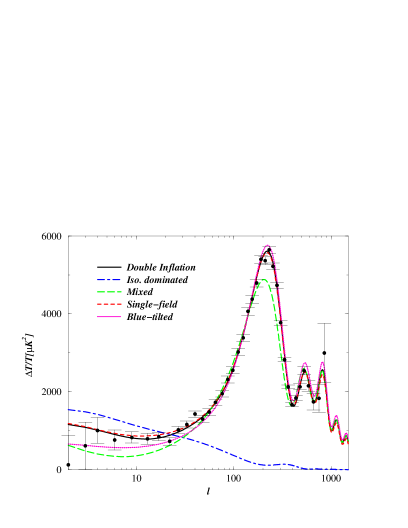
Figure 8: The CMB angular power spectra for the double inflation model (32) with $g^{2}/\lambda=2$ Parkinson04 for five different cases:
(i) the best-fit double inflation model,
(ii) isocurvature dominating over the adiabatic,
 (iii) the isocurvature is comparable to the adiabatic (mixed),
(iv) the best fit single-field model with potential $V=(\lambda/4)(\chi^{2}-M^{2}/\lambda)^{2}$ and
(v) a model with blue-tilted spectrum ($n_{\cal R}>1$) on large scales.

Physical models for the origin of the primordial perturbations may give distinctive predictions for the amplitude and correlation of isocurvature matter perturbations, such as the curvaton and modulated reheating models that we will discuss later.

VIII.2 Neutrino isocurvature modes

The primordial cosmic fluid includes photons, baryons, cold dark matter and neutrinos. The neutrinos may also have a density perturbation relative to the photons, given from Eq. (83) as

$${\cal S}_{\nu}=\frac{3}{4}\left(\frac{\delta\rho_{\nu}}{\rho_{\nu}}-\frac{\delta\rho_{\gamma}}{\rho_{\gamma}}\right)\,,$$ (228)

for relativistic neutrinos (which we shall assume hereafter). Like the matter isocurvature perturbations this produces a series of acoustic peaks out of phase with the adiabatic case.

Because neutrinos only decouple from the photons shortly before primordial nucleosynthesis it is not easy to introduce an isocurvature perturbation relative to the photons. It may only be possible in models with a significant lepton asymmetry, $\xi_{\nu}$. In this case the neutrino density before decoupling is determined not just by the photon temperature but also a non-zero chemical potential. This is possible in some curvaton models Lyth03p2 , but the net lepton asymmetry is now tightly constrained by observations which require the neutrino degeneracy parameter $|\xi_{\nu}<0.07|$ for all flavours Dolgov02 .

For relativistic particles such as neutrinos it is also possible to consider a relative velocity perturbation which is non-singular in the early time limit in the synchronous gauge Bucher99 (though the longitudinal gauge potential $\Phi$, for instance, is singular). Because this is a relative velocity perturbation, not a relative density perturbation, it produces acoustic oscillations out of phase with the isocurvature density perturbations, but approximately in phase with the adiabatic mode.

When one considers the most general primordial perturbation, including all isocurvature modes and their correlations it becomes much harder to exclude the possibility of a significant isocurvature contribution to the CMB angular power spectrum Moodley04 . This is mainly due to the neutrino isocurvature velocity mode and there is no theoretical model of how a scale invariant spectrum for such a mode could be generated.

IX Reheating the universe after inflation

At the end of inflation the universe is typically, but not always , in a highly non-thermal state - and a very cold one at that. The key ability of inflation to homogenise the universe also means that it leaves the cosmos at effectively zero temperature and hence any successful theory of inflation must also explain how the cosmos was reheated - or perhaps defrosted - to the high temperatures we require for the standard hot Big Bang picture. At the very least this must include baryogenesis and nucleosynthesis. Baryogenesis requires energies greater than the electroweak scale but is very model-dependent and is known to require out-of-equilibrium processes. But primordial nucleosynthesis requires that the universe is close to thermal equilibrium at a temperature around 1 MeV.

One of the key realisation of the past few years has been that the process of reheating can have a profound impact on the cosmological predictions of the preceding inflationary phases, as we will discuss in sections XI and XII. In addition our understanding of the process by which inflation ends and reheating takes place has undergone significant advances recently, which we now review.

The so-called “old” theory of reheating, developed in the immediate wake of the first inflationary theories abbott82 ; DL82 , was based on the concept of single-body decays. In this picture the inflaton field is a collection of scalar particles each with a finite probability of decaying, just as a free neutron decay into a proton, electron and anti-neutrino. Such decays can be treated by coupling the inflaton, $\phi$, to other scalar ($\chi$) or fermion ($\psi$) fields through terms in the Lagrangian such as $\nu\sigma\phi\chi^{2}$ and $h\phi\overline{\psi}\psi$. Here $\sigma$ has the dimensions of mass and $\nu$ and $h$ are dimensionless couplings.

Dimensional analysis allows one to estimate the tree-level decay rates ($\Gamma$) for these two interactions since $[\Gamma]=t^{-1}=m$. When the mass of the inflaton is much larger than those of $\chi$ and $\psi$ ($m_{\phi}\gg m_{\chi},m_{\psi}$), the decay rate is DL82 ; Lindebook

$$\Gamma_{\phi\rightarrow\chi\chi} = \frac{\nu^{2}\sigma^{2}}{8\pi m_{\phi}}\,,$$ (229)

$$\Gamma_{\phi\rightarrow\psi\overline{\psi}} = \frac{h^{2}m_{\phi}}{8\pi}\,.$$ (230)

From this we can estimate the temperature at which the universe will reach thermal equilibrium since until $\Gamma>H$ the expansion will not allow a thermal distribution to be reached. This implies that an upper limit on the temperature after inflation is given by solving $\Gamma_{{\rm tot}}\equiv\Gamma_{\phi\rightarrow\chi\chi}+\Gamma_{\phi\rightarrow\psi\overline{\psi}}=H=(8\pi\rho/3m_{\rm pl}^{2})^{1/2}$ for the temperature. Assuming all the energy density $\rho$ of the universe is in the form of relativistic matter with $\rho\simeq g_{*}\pi^{2}T^{4}/30$ where $g_{*}$ is the effective number of massless degrees of freedom ($g_{*}=10^{2}$-$10^{3}$), we obtain the reheat temperature, $T_{{\rm rh}}$:

$$T_{{\rm rh}}\simeq 0.2\left(\frac{100}{g_{*}}\right)^{1/4}\sqrt{\Gamma_{{\rm tot}}m_{{\rm pl}}}\,.$$ (231)

Note that if there is a significant amount of massive particles (with number density evolving as $a^{-3}$), not in the form of radiation, then the reheat temperature is modified since the dependence of $H$ on $T$ is altered.

Neglecting this case, let us impose the constraint that comes from the normalisation of the CMB on large scales; namely that $m_{\phi}\sim 10^{-6}m_{{\rm pl}}$. This ensures that the models do not over-produce anisotropies in the CMB. Requiring that radiative corrections mediated by the couplings do not spoil the flatness of the potential limits the reheat temperature to be below the GUT scale, $T_{{\rm rh}}<10^{16}{\rm GeV}$, which means that the GUT symmetries are not restored and hence there is not a second phase of production of monopoles that inflation was introduced to solve in the first place! However, this does not mean there are no problems. If one is building models of inflation in a supergravity context then one must worry about the over-production of gravitinos, the supersymmetric partner of the graviton. For a wide range of gravitino masses the reheat temperature must be below $10^{9}\,{\rm GeV}$ in order not to ruin the standard successes with nucleosynthesis (e.g., ellis84 ; KM95 ; moroi95 ). Similar constraints come from other dangerous relics which can overclose the universe or release unwanted entropy by decaying around nucleosynthesis.

It is important to note that $T_{\rm rh}$ is not necessarily the largest temperature reached in the history of the universe and in some cases the temperature can be much higher Giudice00 or plasma effects may renormalise the masses of the decay products $\chi$ and $\psi$, meaning that the inflaton may be kinematically forbidden to decays Kolb03 . In this case the reheat temperature is independent of the couplings $h,\nu$ and depends only on $m_{\phi}$. The lesson we learn from this is that effective masses, which differ from the bare particle mass either through classical couplings or quantum corrections, can have a powerful effect on the dynamics of the system. This insight, together with the insight that effective masses can be time and space dependent, is one of the main insights of the 1990’s in inflationary cosmology and is at the heart of preheating.

X Preheating

The majority of the inflaton energy at the end of inflation is homogeneous, stored in the $k=0$ mode of the inflaton. If the inflaton potential has a minimum, such as in simple chaotic inflation models given by Eq. (25), this energy oscillates perfectly coherently (at least at zero order) in space. It is this coherence which is key to preheating. Consider the archetypal massive, chaotic inflaton potential:

$$V(\phi)=\frac{1}{2}m_{\phi}^{2}\phi^{2}\,.$$ (232)

Under the influence of this potential, the homogeneous part of the inflaton simply executes oscillations around $\phi=0$ which gradually decay due to the expansion of the universe:

$$\phi(t)=\bar{\phi}(t)\sin(m_{\phi}t)\,,~{}~{}~{}\bar{\phi}(t)=\frac{m_{\rm pl}}{\sqrt{3\pi}m_{\phi}t}\,.$$ (233)

Here $\bar{\phi}(t)$ is the amplitude of inflaton oscillations which decreases in time. The end of inflation is estimated as $\phi_{f}=m_{{\rm pl}}/2\sqrt{\pi}$ when the slow-roll parameter $\epsilon$ becomes unity. The initial amplitude for the oscillation of the field $\phi$ is slightly smaller than $\phi_{f}$, i.e., $|\phi_{0}|\sim 0.2m_{{\rm pl}}$ KLS97 .

Since the occupation number of the inflaton $k=0$ mode (the homogeneous part of the inflaton) is very large at the end of inflation it behaves essentially as a classical field. One can therefore, to first approximation, treat the inflaton as a classical external force acting on the quantum fields $\chi$ and $\psi$. Because the inflaton is time-dependent, the effective masses of $\chi$ and $\psi$ change very rapidly. Then this leads to the non-adiabatic excitation of the field fluctuations by parametric resonance. As a result, the picture we had before of the inflaton as a large collection of statistically independent particles breaks down and the spatial and temporal coherence of the inflaton can cause radical departures from the “old” theory of reheating described in the previous section. This is the essence of preheating TB90 ; Dolgov82 , STB94 ; KLS94 (see also Refs. KT1 ; KT2 ; KT3 ; Yoshi ; Boy96 ; Boy97 ; PR97 ; Son ; Baacke97 ; KLS97 ).

For simplicity, let us consider the coupling of the inflaton to the scalar $\chi$ only, through an interaction term in the Lagrangian of the form $(1/2)g^{2}\phi^{2}\chi^{2}$ where $g$ is a dimensionless coupling that will play a key role in our analysis. Classically this does not describe the single-body decay of the inflaton, but rather the process in which two $\phi$ bosons interact and decay into two $\chi$ particles. The total effective potential for this system will be the sum of the potential driving inflation which for simplicity we assume is independent of $\chi$, $V(\phi)$, and the above interaction term:

$$V_{{\rm eff}}(\phi,\chi)=V(\phi)+\frac{1}{2}g^{2}\phi^{2}\chi^{2}\,,$$ (234)

which corresponds to a $\chi$ field with zero bare mass but with an effective mass given by

$$m_{\chi,{\rm eff}}^{2}\equiv\frac{\partial^{2}V_{{\rm eff}}(\phi,\chi)}{\partial\chi^{2}}=g^{2}\phi^{2}(t)\,.$$ (235)

A base mass for the $\chi$ field, $m_{\chi}$ can be accommodated simply into the above expression by adding $m_{\chi}^{2}$. Equation (235) is the appropriate notion of effective mass for the $\chi$ field because, neglecting metric perturbations for the moment, the Fourier modes of the $\chi$ field obey a modified Klein-Gordon equation

$$\ddot{\chi}_{k}+3H\dot{\chi}_{k}+\left[\frac{k^{2}}{a^{2}}+g^{2}\phi^{2}(t)\right]\chi_{k}=0\,,$$ (236)

with $m_{\chi,{\rm eff}}^{2}$ playing the crucial role of mass in the equation.

This is a radical point of view since we now are asking for the quantum dynamics of the field with a time-dependent mass. From the point of view of solving ordinary differential equations, this equation resembles that of a damped ($H\neq 0$) harmonic oscillator with a time-dependent mass.

From WKB theory we know that if the frequency, $\omega_{k}\equiv[k^{2}/a^{2}+g^{2}\phi^{2}(t)]^{1/2}$, is varying slowly with time, then the solution to this equation is close to those of the equation in which $\omega_{k}^{2}$ is constant. In this case it is well known that the solutions $\chi_{k}(t)$ do not grow, which corresponds physically to saying that there is no production of $\chi$ particles. If, on the other hand, the effective mass is changing rapidly, then WKB analysis breaks down. This is quantified by the dimensionless ratio

$$R_{a}\equiv\frac{\dot{\omega}_{k}}{\omega_{k}^{2}}\,.$$ (237)

The regime $|R_{a}|\ll 1$ is often known as the adiabatic region since in this case the particle number, $n_{k}$, is an adiabatic invariant which does not change in time and encapsulates the idea that there is no particle production. In the region $|R_{a}|\gg 1$ the particle number is no longer an adiabatic invariant and we can expect significant particle production. The standard estimate of the comoving occupation number of bosons in mode $k$ is KLS97 :

$$n_{k}=\frac{\omega_{k}}{2}\left(\frac{|\dot{X}_{k}|^{2}}{\omega_{k}^{2}}+X_{k}^{2}\right)-\frac{1}{2}\,,$$ (238)

where $X_{k}\equiv a^{3/2}\chi_{k}$. Eq. (238) can be justified, at least qualitatively, as the ratio of the energy in mode $k$, (the sum of the “kinetic energy” $\dot{X}_{k}^{2}$ and the “potential energy” $\omega_{k}^{2}X_{k}^{2}$), divided by the energy per particle, $\omega_{k}$. It clearly shows how the number of particles is clearly linked to the amplitude of the mode, $X_{k}$.

For the interaction in (235), and for long wavelengths $k/aH\ll 1$, the dimensionless ratio $R_{a}$ is given approximately by

$$R_{a}\simeq\frac{\dot{\phi}}{g\phi^{2}}\sim\frac{m_{\phi}}{g\phi}\,,$$ (239)

where in the second equality we have assumed $\dot{\phi}\sim m_{\phi}\phi$ which is suitable for most periodic oscillations of the inflaton after inflation. The key point about this relation is that $R_{a}$ diverges whenever $\phi\rightarrow 0$, i.e. at every oscillation! Hence we can expect rampant particle production around every oscillation of the inflaton.

From Eq. (236) the equation for $X_{k}$ can be formally put in the form of the so-called Mathieu equation Mathieu

$$\frac{{\rm d}^{2}X_{k}}{{\rm d}z^{2}}+\left(A_{k}-2q\cos 2z\right)X_{k}=0\,,$$ (240)

where $z=m_{\phi}t$ is the natural dimensionless time and

$$A_{k}=2q+\frac{k^{2}}{m_{\phi}^{2}a^{2}}\,,~{}~{}~{}q=\frac{g^{2}\bar{\phi}^{2}(t)}{4m_{\phi}^{2}}\,.$$ (241)

In deriving this we neglected the term $-(3/4)(2\ddot{a}/a+\dot{a}^{2}/a^{2})$, which is not important relative to the $g^{2}\phi^{2}$ term during preheating. From Eq. (241) the allowed range of $A_{k}$ and $q$ corresponds to $A_{k}\geq 2q$.

The strength of resonance depends upon the variables $A_{k}$ and $q$, which is described by a stability-instability chart of the Mathieu equation Mathieu ; KLS94 . Formally $A_{k}$ and $q$ should be constant to use the Mathieu equation but as long as they are not varying too rapidly the analogy is reasonable.

According to Floquet theory, when $A_{k},q$ fall in an instability band, the perturbation $X_{k}$ grows exponentially with a Floquet index $\mu_{k}>0$, i.e., $X_{k}\propto{\rm exp}(\mu_{k}z)$. For small $q~{}(\mbox{\raisebox{-4.30554pt}{$\stackrel{{\scriptstyle\textstyle<}}{{\textstyle\sim}}$}}~{}1)$ the width of the instability band is small and the expansion of the universe washes out the resonance. On the other hand, for the large $q~{}(\gg 1)$, broad resonance can occur for a wide range of the parameter space and momentum modes.

Note that the initial amplitude $\phi_{0}$ of the inflaton and the coupling $g$ play important roles in determining whether resonance is efficient or not. Since the inflaton mass is constrained to be $m_{\phi}\sim 10^{-6}m_{\rm pl}$ by the COBE normalization, large resonance parameters, $q\gg 1$, can be easily achieved for the coupling $g~{}\mbox{\raisebox{-4.30554pt}{$\stackrel{{\scriptstyle\textstyle>}}{{\textstyle\sim}}$}}~{}10^{-4}$ with an initial amplitude, $\phi_{0}\sim 0.2m_{\rm pl}$.

For $q\gg 1$, particle production only occurs near $\phi=0$. Hence we may Taylor expand the $\chi$ effective mass around this point and keep only the quadratic F96 ; KLS97 , $\phi=\alpha(t-t_{j})$ where $\phi(t_{j})=0$ for $j=1,2,3...$ and $\alpha$ is a coefficient that depends on the specific potential one is studying. For the quadratic potential, Eq. (236) becomes the equation of a particle scattering in a parabolic potential:

$$\frac{{\rm d}^{2}X_{k}}{{\rm d}t^{2}}+\left[\frac{k^{2}}{a^{2}}+g^{2}\alpha^{2}(t-t_{j})^{2}\right]X_{k}=0\,,$$ (242)

where $\alpha=m\bar{\phi}$. The general solution to Eq. (242) F96 ; KLS97 can be written as a linear combination of the parabolic cylinder functions $W(-\kappa^{2}/2;\pm\sqrt{2}k_{*}(t-t_{j}))$ where

$$\kappa^{2}\equiv\frac{k^{2}}{(ak_{*})^{2}}\,,$$ (243)

and $k_{*}^{2}\equiv gm_{\phi}\bar{\phi}$.

Since the evolution of the inflaton is periodic, the problem is that of repeated barrier penetration and we can use the exact solution to estimate the Floquet index, $\mu^{j}_{k}$ (the exponent by which the modes, $X_{k}$ grow, i.e. $\mu_{k}^{j}=\ln(\Delta X_{k}/\Delta t)$ at each scattering, $j$)KLS97 :

$$\mu_{k}^{j} = \frac{1}{2\pi}\ln\left[1+2E-2\sin\theta^{j}_{tot}\sqrt{E(1+E)}\right]\,,$$

$$E \equiv e^{-\pi\kappa^{2}}\,,$$ (244)

where $\kappa^{2}$ is the dimensionless wavenumber defined by Eq. (243) and $\theta_{tot}^{j}$ is the phase of the wavefunction which changes quantum mechanically at each scattering in the parabolic potential. This expression shows how particle production decreases exponentially with increasing frequency, $k$ and how the phase can significantly alter the Floquet index $\sin\theta_{tot}$.

In Ref. KLS97 it was further noticed that while in Minkowski spacetime the phase is independent of time, this is not true in an expanding background and in fact the change in phase between successive scatterings, $\delta\theta_{k}\simeq\sqrt{q}/\tilde{N}^{2}$ where $\tilde{N}$ is the number of inflaton oscillations. (For more discussion of the phase dynamics see Ref. CNM .) The requirement $\delta\theta_{k}>2\pi$ defines a region of time and parameter space during which the phase behaves as a quasi-random number generator . Hence the value of the Floquet index changes effectively stochastically from one oscillation of the inflaton to another. This has become known as stochastic resonance KLS97 . We caution that this is different from the term stochastic resonance as used in control theory and condensed matter physics which is now a well-established experimental field, e.g., stocres .

From this formalism we can also illustrate a crucial point about the non-perturbative nature of the particle production in preheating. If decays of the inflaton are perturbative, it is obvious that an inflaton boson at rest cannot decay to a particle which has more mass than the inflaton, this is kinematically forbidden. In preheating this is not true. Particles with masses larger than the inflaton mass can be produced.

To see this, consider the expression for $R_{a}$, in Eq. (239), but this time include a bare mass for the $\chi$ field, $m_{\chi}$. Proceeding as before gives:

$$R_{a}\simeq\frac{m_{\phi}g^{2}\phi^{2}}{(m^{2}_{\chi}+g^{2}\phi^{2})^{3/2}}\,.$$ (245)

In this case (at least for $g^{2}>0$) $R_{a}$ can no longer diverge, even in the $k\rightarrow 0$ limit and indeed now vanishes at $\phi=0$ (see Fig. 9). However non-adiabatic particle creation occurs provided $m_{\chi}<|g\phi|$ (similar properties hold in producing particles at large momentum, $k$). When $g^{2}<0$, $R_{a}$ can still diverge formally and in this case production of extremely massive particles is possible, although care must be taken so that the total potential is bounded from below.

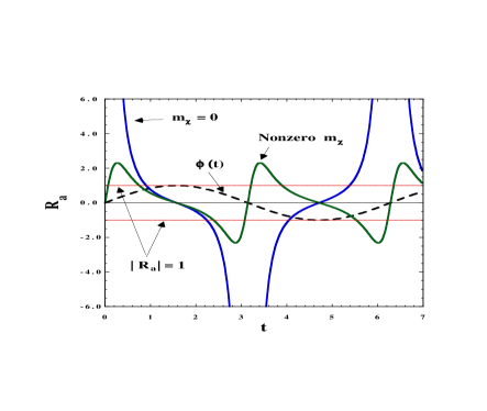
Figure 9: $\phi(t)$ and the dimensionless ratio $R_{a}\equiv\dot{\omega}_{k}/\omega^{2}_{k}$ for the massive model for $m_{\chi}=0$ and an arbitrary value of $m_{\chi}>0$. While $R_{a}$ diverges at $\phi=0$ for the massless case, it vanishes at $\phi=0$ for the massive case. Particle production takes place in the non-adiabatic region characterised by $|R_{a}|>1$. Massive particles can be created provided that the maximum value of $|R_{a}|$ is larger than 1.

X.1 The conformally invariant case

There is an interesting exactly solvable special model worth mentioning in which the expansion of the universe can be transformed away and exact Floquet theory is applicable. This is the conformally invariant potential

$$V_{\rm eff}(\phi,\chi)=\frac{1}{4}\lambda\phi^{4}+\frac{1}{2}g^{2}\phi^{2}\chi^{2}\,.$$ (246)

In this model the universe rapidly becomes radiation dominated ($a\propto t^{1/2}\propto\tau$, where $\tau$ is a conformal time). The homogeneous part of the inflaton obeys the equation of motion

$$\frac{{\rm d}^{2}\varphi}{{\rm d}x^{2}}+\lambda\varphi^{3}=0\,,$$ (247)

where $\varphi\equiv a\phi$ and $x\equiv\sqrt{\lambda}\varphi_{0}\tau$ with $\varphi_{0}$ being the initial amplitude of the oscillations of the conformal field $\varphi$. Note that this equation is that of an harmonic oscillator in flat space - the expansion of the universe has been absorbed into the field and time redefinitions. The solution to this is the Jacobi cosine function

$$\varphi=\varphi_{0}\mbox{cn}\left(x;\frac{1}{\sqrt{2}}\right)\,,$$ (248)

which is closely approximated by $\varphi_{0}\cos(0.8472x)$ GKLS97 .

One can show that the equation of motion for $X_{k}\equiv a\chi_{k}$ in conformal time is also just that of a field in Minkowski spacetime with all the effects of the expansion absorbed into the field and time redefinitions:

$$\frac{{\rm d}^{2}}{{\rm d}x^{2}}X_{k}+\left[\kappa^{2}+\frac{g^{2}}{\lambda}{\rm cn}^{2}\left(x;\frac{1}{\sqrt{2}}\right)\right]X_{k}=0\,,$$ (249)

where $\kappa^{2}\equiv k^{2}/(\lambda\varphi_{0}^{2})$. This equation is the so-called Lamé equation. The advantage of converting the equations into Minkowski form is that the coefficients appearing in Eq. (249) are now exactly periodic in time and hence one can use the theorems of Floquet theory to show that there must be exponentially growing solutions, $X_{k}\propto e^{\mu x}$ where the Floquet index varies between zero and a maximum value $\mu_{max}\simeq 0.238$ as a function of ${\kappa}$ and $g^{2}/\lambda$ Kaiser97 ; Kaiser98 ; GKLS97 .

The structure of resonance is completely determined by the value of the parameter $g^{2}/\lambda$. One can expect an efficient particle production even for small couplings, $g^{2}/\lambda\sim{\cal O}(1)$. The long-wave modes ($\kappa\to 0$) are enhanced in the intervals $n(2n-1)<g^{2}/\lambda<n(2n+1)$ with $n$ being a positive integer. The centre of the resonance bands corresponds to $g^{2}/\lambda=2n^{2}=2,8,18,\cdots$, around which parametric resonance is efficient. Figure 10 shows that there are upper limits of the momenta which are amplified by parametric resonance, depending on the values of $g^{2}/\lambda$.

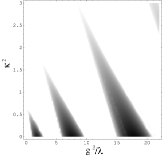
Figure 10: Density plot of the Floquet chart for the Lamé equation (249) for $0\leq g^{2}/\lambda\leq 22$ and $\kappa^{2}\leq 3$. The shaded regions correspond to parameter ranges in which parametric resonance occurs, $\mu_{k}>0$. The Floquet index, $\mu_{k}$, takes larger values in the darker shaded regions, and reaches its maxima for $g^{2}/\lambda=2n^{2}$ at $\kappa^{2}=0$.

The perturbation equation for inflaton can be written as

$$\frac{{\rm d}^{2}}{{\rm d}x^{2}}\delta\varphi_{k}+\left[\kappa^{2}+3{\rm cn}^{2}\left(x;\frac{1}{\sqrt{2}}\right)\right]\delta\varphi_{k}=0\,,$$ (250)

where $\delta\varphi_{k}\equiv a\delta\phi_{k}$. This corresponds to $g^{2}/\lambda=3$ in Eq. (249). The perturbations $\delta\varphi_{k}$ grow provided that the momenta exist in the range Kaiser97 ; Kaiser98 ; GKLS97 :

$$\frac{3}{2}<\kappa^{2}<\sqrt{3}\,.$$ (251)

The maximum growth rate for $\delta\varphi_{k}$ is found to be $\mu_{{\rm max}}\approx 0.03598$ at $\kappa^{2}\approx 1.615$. It is interesting that preheating occurs for the quartic model even in the absence of the $\chi$ field. However the modes which are amplified are at sub-Hubble scales (251) for the inflaton fluctuations. We will understand this later as due to the fact that the entropy perturbation in single-field models decays as $k^{2}$ on large scales.

X.2 Geometric preheating

In previous subsections, we considered the standard scenario of preheating where inflaton $\phi$ is coupled to $\chi$ through an interaction, $(1/2)g^{2}\phi^{2}\chi^{2}$. From the viewpoint of quantum field theories in curved spacetime, non-minimal couplings naturally arise, with their own nontrivial renormalization group flows. The ultra-violet fixed point of these flows are often divergent, implying that non-minimal couplings may be important in the early universe. This provides an alternative - geometric - channel for resonance BL97 ; TMT99 in which scalar fields coupled to the scalar curvature $R$ which oscillates during reheating.

Let us consider an inflaton field $\phi$ interacting with a scalar field $\chi$, which is non-minimally coupled to gravity:

$${\cal L}=\sqrt{-g}\biggl{[}\frac{m_{\rm pl}^{2}}{16\pi}R - \frac{1}{2}(\nabla\phi)^{2}-\frac{1}{2}m_{\phi}^{2}\phi^{2}-\frac{1}{2}(\nabla\chi)^{2}$$ (252)

$$- \frac{1}{2}g^{2}\phi^{2}\chi^{2}-\frac{1}{2}\xi R\chi^{2}\biggr{]}\,.$$

Then the equation for the perturbation $\delta\chi_{k}$ reads

$$\ddot{\delta\chi}_{k}+3H\dot{\delta\chi}_{k}+\left(\frac{k^{2}}{a^{2}}+g^{2}\phi^{2}+\xi R\right)\delta\chi_{k}=0\,.$$ (253)

The scalar curvature, $R=6(2H^{2}+\dot{H})$, oscillates during reheating. Making use of the time-averaged relation $\langle m_{\phi}^{2}\phi^{2}\rangle=\langle\dot{\phi}^{2}\rangle$, we find that $R\sim 8\pi m_{\phi}^{2}\phi^{2}/m_{\rm pl}^{2}$. Then the contribution of the $\xi R$ term becomes more important than that of the $g^{2}\phi^{2}$ term when the coupling satisfies the condition

$$\frac{|\xi|}{g^{2}}\gtrsim\frac{1}{8\pi}\left(\frac{m_{\rm pl}}{m_{\phi}}\right)^{2}\,.$$ (254)

When $g\gtrsim 10^{-4}$, the condition (254) corresponds to $|\xi|\gtrsim 10^{2}$. It was found that parametric resonance occurs for negative non-minimal couplings of order $|\xi|\sim 1$ provided that non-gravitational coupling is smaller than of order $g=10^{-5}$. Thus the geometric particle production can provide an alternative scenario of preheating even when the non-gravitational interaction is negligible.

X.3 Almost-periodic and random parametric resonance

So far we have considered simple potentials with periodic evolution of the $\chi$ effective mass modulated by powers of $a$. What happens if we consider more general evolution of the effective mass? For example, what happens if the effective mass² behaves as:

$$m_{\chi,{\rm eff}}^{2}\propto g_{1}^{2}\cos(\omega_{1}t)+g_{2}^{2}\cos(\omega_{2}t)\,,$$ (255)

with $\omega_{1}/\omega_{2}$ irrationally related? In this case the function is not exactly periodic. Or what happens if the effective mass evolves with a random component or stochastically in time?

Given our general criterion $R_{a}>1$ in Eq. (239) for resonance we should suspect that exponential growth of $\chi_{k}$ modes should be possible in certain cases, and this is indeed the case. One way to show this is to note that there is a duality between the temporal evolution of $\chi_{k}$ modes and the 1-dimensional time-independent Schrödinger equation which relates the wavenumber $k$ to the eigenvalues $\lambda$ and interchanges space and time. Then, the modes $k$ which grow exponentially correspond to the complement of the spectrum of allowed eigenvalues.

This immediately explains why the exponentially growing modes in the periodic case belong to bands. These are, in the dual picture, just the complement of the usual Bloch conduction bands that characterise the allowed energy levels of periodic lattice structures in metals.

Using this insight, and results from the spectral theory of the Schrödinger operator, we can show that in the case of almost-periodic and similar evolution, the $\chi_{k}$ modes do not experience resonance (have vanishing Floquet index $\mu_{k}=0$) only on a nowhere dense (Cantor) set BB98 ; Zanchin98 ; Zanchin99 . Hence, generically resonance occurs at all wavelengths, not just in certain resonance bands.

Similar results hold for random evolution of the $\chi$ effective mass. In this case one can rigorously show that for sufficiently random evolution the Floquet index $\mu_{k}$ is strictly positive for all $k$ except on a set of measure zero BB98 ; Zanchin98 ; Zanchin99 . In the case $m_{\chi,{\rm eff}}^{2}=\kappa^{2}+q\xi(t)$ where $\kappa^{2}$ and $q$ are dimensionless constants and $\xi(t)$ is a mean-zero, ergodic Markov process, perturbative expansion gives BB98 ; Zanchin98 ; Zanchin99

$$\mu_{k}=\frac{\pi}{4}\frac{q^{2}}{\kappa^{2}}\hat{f}(2\kappa)+{\cal O}(q^{3})\,,$$ (256)

where $\hat{f}(\kappa)$ is the Fourier transform of the expectation value of the two-time correlation function $\langle\xi(t)\xi(t-t^{\prime})\rangle$. Hence, a mode $k$ will grow exponentially if the Fourier transform is non-zero at twice the frequency. In the case where the noise is delta-correlated, then $\langle\xi(t)\xi(t-t^{\prime})\rangle\propto\delta(t-t^{\prime})$ and $\hat{f}(\kappa)={\rm const}.$ and all modes grow exponentially. Temporal correlations (coloured noise) mean that the Fourier transform has compact support and hence removes the resonance for sufficiently large frequencies.

This result has a celebrate condensed matter analogue - Anderson localisation, which states that with small random impurities, eigenfunctions become exponentially localised. In the case of reheating, these results mean that periodic evolution is actually the most modest. By studying the conformal case we can extend these results to an expanding FRW background. Since white noise is a well-studied limit of chaotic motion these results also provide insight into preheating in cases where the inflaton evolves chaotically BT98 .

X.4 Tachyonic preheating and the negative coupling instability

So far we have always considered the case $m_{\chi,{\rm eff}}^{2}>0$. However it was realised in Ref. negci that the coupling $g^{2}\phi^{2}\chi^{2}/2$ in Eq. (234) could just as well be replaced by $g\phi^{2}\chi^{2}/2$ with $g<0$ if the potential was supplemented by additional terms ($\propto\chi^{4},\phi^{4}$) that ensured that the full potential was bounded from below. In this case, the $\chi$ effective mass squared is $m_{\chi,{\rm eff}}^{2}\sim g\phi^{2}$ which can be negative, implying that there can be tachyonic phases. Crucially this negative coupling instability implies that many more modes are resonantly amplified compared with standard preheating (with $g^{2}>0$) and the corresponding Floquet indices, $\mu_{k}$ can be much larger, allowing for the production of very massive $\chi$ particles that may be relevant for baryogenesis negci .

Tachyonic instabilities inevitably occur in models of spontaneous symmetry breaking. In particular $m^{2}_{\chi,{\rm eff}}$ becomes negative in the hybrid inflation model given by Eq. (32) when the $\phi$ field drops below the critical value $\phi_{c}=M/g$ at the end of inflation. Long-wavelength modes initially grow due to the tachyonic (spinodal) instability, but non-linear effects rapidly become important Felder01p1 ; Felder01p2 . The existence of non-perturbative features such as topological defects has a profound impact on the time taken for backreaction to end preheating. Instead of taking multiple oscillations it was found that resonance ends very rapidly, after only ${\cal O}(1)$ oscillations; a process dubbed “tachyonic preheating” Felder01p1 . In the case of a $Z_{2}$ symmetry with two vacua at $\phi=\pm v$, the universe is divided into regions of $\phi=\pm v$, separated by domain walls. The gradient energy associated with this non-perturbative field configuration is comparable to the initial potential energy of the field before symmetry breaking. The gradients contribute very strongly to the variance $\langle\delta\phi^{2}\rangle$ which quells the resonance very rapidly. The reader is referred to Felder01p1 ; Felder01p2 for more details.

X.5 Fermionic preheating

Quite soon after the initial studies of preheating of scalar fields attention turned to the possibility of resonant production of fermions. This is an important issue since many problematic particles such as gravitinos, are fermions and resonant production of them could have a profound impact on dangerous relic abundances Baacke98 ; GK98 .

Nevertheless fermions obey the exclusion principle which implies that $n_{k}\leq 1$ so the system is severely constrained. Consider the conformally coupled inflaton interacting with a massless fermion field $\psi$ through the interaction term $h\phi(t)\overline{\psi}\psi$ where $h$ is the dimensionless Yukawa coupling. The resulting Dirac equation to first order in a flat FRW background is Baacke98 ; GK98

$$[i\gamma_{\mu}\nabla^{\mu}-m_{\rm eff}]\psi=0\,,$$ (257)

where $\gamma_{\mu}$ are the Dirac matrices and the effective mass is given by

$$m_{{\rm eff}}=m_{\psi}+h\phi(t)\,.$$ (258)

Here $m_{\psi}$ is the bare mass of fermions. As in the scalar case, the coupling to the homogeneous part of the inflaton acts as a time-dependent effective mass $m_{{\rm eff}}$.

Let us consider the self-coupling inflaton potential $V(\phi)=(1/4)\lambda\phi^{4}$. We introduce a conformally rescaled field $\tilde{\psi}=a\psi$ and decompose the field $\tilde{\psi}$ into Fourier components as

$$\tilde{\psi} = \frac{1}{(2\pi)^{3/2}}\int d^{3}k\sum_{s}[a_{s}(k)\tilde{{\bf u}}_{s}(k,\eta)e^{+i{\bf k}\cdot{\bf x}}$$

$$+b_{s}^{\dagger}(k)\tilde{{\bf v}}_{s}(k,\eta)e^{-i{\bf k}\cdot{\bf x}}]\,.$$

Imposing the following standard ansatz GK98 :

$$\tilde{{\bf u}}_{s}(k,\eta)=(-i\gamma^{\mu}\partial_{\mu}-m_{\rm eff}a)\tilde{\psi}_{k}(t)W_{\pm}(k)\,,$$ (260)

where $W_{\pm}(k)$ are the eigenvectors of the helicity operator, which satisfy the relation $\gamma^{0}W_{\pm}(k)=1$ and ${\bf k}\cdot\sum W_{\pm}(k)=\pm 1$, we obtain the mode equation for the $\tilde{\psi}_{k}$:

$$\left[\frac{{\rm d}^{2}}{{\rm d}x^{2}}+\kappa^{2}+f^{2}-i\frac{{\rm d}f}{{\rm d}x}\right]\tilde{\psi}_{k}=0\,,$$ (261)

where

$$f\equiv\frac{m_{\rm eff}a}{\sqrt{\lambda}\phi(0)},~{}~{}~{}\kappa^{2}\equiv\frac{k^{2}}{\lambda\phi^{2}(0)},~{}~{}~{}x\equiv\sqrt{\lambda}\phi(0)\eta\,.$$ (262)

Here $\phi(0)$ is the initial value of inflaton at the onset of preheating. Equation (261) bears a striking resemblance to the Klein-Gordon equation except for the appearance of the complex term $i{\rm d}f/{\rm d}x$ in the effective mass. This is to be expected since the Klein-Gordon equation expresses relativistic energy momentum conservation which must also apply to fermions. The complex term appears as the enforcer of the Pauli exclusion principle.

Equation (261) has a WKB-form solution given in terms of creation and annihilation operators by

$$\tilde{\psi}_{k} = \alpha_{k}N_{+}\exp\left(-i\int_{0}^{t}\Omega_{k}{\rm d}x\right)$$ (263)

$$+\beta_{k}N_{-}\exp\left(+i\int_{0}^{t}\Omega_{k}{\rm d}x\right)\,,$$

where $\Omega_{k}^{2}\equiv\kappa^{2}+f^{2}$ and $N_{\pm}\equiv 1/\sqrt{2\Omega_{k}(\Omega_{k}\pm f)}$. The comoving number density of produced fermions is given in terms of the Bogoliubov coefficients $\beta_{k}$ by GK98 ; Tsuji00

$$n_{k}\equiv|\beta_{k}|^{2}=\frac{1}{2}-\frac{\kappa^{2}}{\Omega_{k}}{\rm Im}\left(\tilde{\psi}_{k}\frac{d\tilde{\psi}_{k}^{*}}{dx}\right)-\frac{f}{2\Omega_{k}}\,,$$ (264)

where ^∗ denotes complex conjugation and Im the imaginary part of the expression. The initial conditions are chosen to be $\alpha_{k}(0)=1$, $\beta_{k}(0)=0$, which corresponds to $n_{k}(0)=0$. The Bogoliubov coefficients satisfy the relation $|\alpha_{k}(t)|^{2}+|\beta_{k}(t)|^{2}=1$, which means that the exclusion principle restricts the number density of fermions to below unity, $n_{k}(t)\leq 1$. It is interesting to consider the limits of $\kappa\rightarrow 0$ in Eq. (264). In this case $n_{k}\rightarrow 0$ irrespective of $q$, reinforcing our earlier discussion that the fermion has no homogeneous component.

Fermions are non-adiabatically created when the effective masses of fermions change rapidly. This takes place around $m_{{\rm eff}}=0$ Giudice99 , corresponding to the inflaton value

$$\phi_{c}=-m_{\psi}/h\,.$$ (265)

When the condition, $m_{\psi}>|h\phi|$, is satisfied at the beginning of reheating, the inflaton does not pass through the resonance point (265). Therefore we require the condition, $m_{\psi}<|h\phi|$, to lead to parametric excitation of fermions. Since inflation ends around $\phi=0.3m_{\rm pl}$, it is possible to generate heavy fermions whose masses are of order $10^{17}$-$10^{18}$ GeV Giudice99 ; PS00 .

When we consider supersymmetric theories such as supergravity, gravitino production can provide us a useful tool to constrain particle physics models in early universe. In a perturbative theory of reheating the thermal production of gravitinos places a constraint $T_{{\rm rh}}\lesssim 10^{9}$ GeV, on the reheating temperature KM95 ; moroi95 . On the other hand non-thermal production of gravitinos during preheating has been extensively studied by many authors MM99 ; Giudice99v2 ; Kallosh99 ; Kallosh00 ; Nilles01 ; Nilles01v2 ; GKM03 . In particular it was found in Ref. Nilles01 that gravitino creation is suppressed relative to the superpartner of the inflaton (inflatino) for a model of two scalar fields including a supersymmetry breaking field.

A similar conclusion has been reached in Ref. GKM03 for a more realistic supergravity inflation model. While these results show that gravitino over-production can be avoided during preheating, further studies of how the mixing occurs between fermionic fields for the full Lagrangian derived from supergravity is required for a complete understanding of the problem.

X.6 Instant preheating

Non-perturbative parametric or stochastic resonance is not the only way that a changing effective mass can lead to interesting effects. Consider a scalar field $\chi$ with a bare mass, $m_{\chi}$ coupled to the inflaton through a term $(1/2)g\phi^{2}\chi^{2}$. The $\chi$ field has an effective mass squared of: $m_{\chi}^{2}+g\phi^{2}$. If $g>0$, the effective mass is always larger than the bare mass. However, if $g<0$, then the effective mass vanishes when $\phi=\pm m_{\chi}/\sqrt{-g}$. As a result the inflaton is kinematically allowed to decay there and the corresponding $R_{a}$ diverges, see Eq. (245).

This insight was used to argue that in so-called distributed-mass models where there are a large number of decay states with a spectrum of masses (as occurs in string theory due to the exponential density of states), the slowly rolling inflaton will successively make each of the states massless and hence will lead to successive bursts of particle production which may be strong enough to sustain warm inflation warm .

Coupling these insights to those of parametric resonance leads to an interesting phenomenology instant . For a coupling $(1/2)g^{2}\phi^{2}\chi^{2}$ of some scalar $\sigma$ and for large $q\gg 1$ we have shown that particle production only occurs in small bursts near $\phi=0$. Now imagine the $\chi$ field is also coupled to a fermion field through an interaction $h\chi\overline{\psi}\psi$. Since these are single body decays, one may use Eq. (230) with $\phi$ replaced by $\chi$. We see that

$$\Gamma_{\chi\rightarrow\overline{\psi}\psi}\simeq\frac{h^{2}g|\phi|}{8\pi}\,.$$ (266)

Hence there is massive resonant production of $\chi$ particles when $\phi\simeq 0$ (during which time $\Gamma_{\chi\rightarrow\overline{\psi}\psi}\sim 0$) followed by $\phi$ oscillating to its maximum at which point the $\chi$ bosons have swelled to maximum effective mass and are most likely to decay. In the first couple oscillations $|\phi|\sim 0.1m_{{\rm pl}}$ and hence the $\chi$ bosons are kinematically allowed to decay to fermion pairs of mass up to $\sim g|\phi|\simeq gm_{{\rm pl}}/10\sim 10^{18}\,{\rm GeV}$ if we allow $g\sim 1$.

Production of particles near the Planck mass is difficult to achieve even for $q\gg 1$ in standard parametric resonance but it is a characteristic feature of instant reheating where large amounts of energy are transferred into massive fermions within a couple of oscillations. We note that instant preheating scenario may be applied to a quintessential inflation in which the potential does not have a minimum, see e.g., SS04 .

X.7 Backreaction and rescattering

So far we have only considered the production of secondary fields ($\chi$, $\psi$) through parametric resonance. Usually in cosmology the perturbations depend on the background dynamics but not vice versa. However, the rapid draining of energy due to the rampant particle production soon affects the dynamics of the inflaton itself. How can this be modelled? We can treat this first by considering the Hartree, or mean-field, approximation KT2 ; KLS97 . In this approximation all effects of the amplification of the $\chi$ field (we consider only the scalar case here) are mediated through the variance of $\chi$, $\langle\chi^{2}\rangle$, and the homogeneous part of the inflaton now obeys the equation:

$$\ddot{\phi}+3H\dot{\phi}+V_{\phi}+g^{2}\langle\chi^{2}\rangle\phi=0\,,$$ (267)

where the variance is defined to be:

$$\langle\chi^{2}\rangle=\frac{1}{2\pi^{2}}\int{\rm d}k\,k^{2}|\chi_{k}|^{2}\,.$$ (268)

Crudely speaking the variance is correlated with the energy in the $\chi$-fluctuations.

Let us consider the quadratic inflaton potential given by Eq. (232). Initially the variance term is vanishingly small, but it grows rapidly according to $\propto e^{2\mu m_{\phi}t}$ (where $\mu$ is some suitable average Floquet index) during preheating and therefore increases the effective mass of the inflaton. We can understand the effect of this increase qualitatively through analogy with a simple harmonic oscillator. Firstly the frequency of $\phi$ oscillations increases and secondly, the approximate conservation of energy means the amplitude of $\phi$ oscillations decreases roughly as $\bar{\phi}\sim m_{\phi,{\rm eff}}^{-1}$. This in turn rapidly decreases the resonance parameter $q\propto\bar{\phi}^{2}/m_{\phi,{\rm eff}}^{2}$, which acts to shut off the resonance, stopping the production of $\chi$ particles.

To estimate the maximum variance that can be achieved one can simple equate the two mass terms in the equation of motion for the condensate, $\phi$. These two terms are $m_{\phi}^{2}$ and $g^{2}\langle\chi^{2}\rangle$ and hence we generally expect $\langle\chi^{2}\rangle_{{\rm max}}\sim m_{\phi}^{2}/g^{2}$. It is clear we are dealing with a non-perturbative process since the coupling $g$ appears in the denominator. When the backreaction of the $\chi$ fluctuations are as large as the inflaton bare mass it is difficult for the resonance to continue much further for the reasons discussed above. The time at which this occurs can be estimated by writing $\langle\chi^{2}\rangle\propto e^{2\mu m_{\phi}t}$, hence

$$t_{{\rm end}}\sim\frac{1}{\mu m_{\phi}}\ln\left(\frac{m_{\phi}}{g}\right)\,.$$ (269)

Again notice the non-perturbative nature of this expression and the logarithmic dependence on the couplings. This comes from the exponential growth of fluctuations which means that the end of the resonance is rather robust in these theories. Nevertheless the Hartree approximation certainly does not give a complete description of preheating because it neglects the fluctuations of the inflaton.

To go beyond the mean-field approximation let us examine the equations of motion in real space. The equations of motion involve products $\phi^{2}({\bf x},t)\chi({\bf x},t)$ and $\phi({\bf x},t)\chi^{2}({\bf x},t)$. We transform them into Fourier space using the convolution theorem which states that the Fourier transform (denoted FT) of a product is the convolution (denoted $*$) of the individual Fourier transforms, i.e.,

$$FT(f\times g)=FT(f)*FT(g)\,,$$ (270)

where the convolution in three dimensions is defined as

$$(f*g)({\bf k})=\int d^{3}k^{\prime}f({\bf k})g({\bf k}-{\bf k}^{\prime})\,.$$ (271)

We can recover the mean-field/Hartree equation (267) by assuming $\phi=\phi(t)$ only, with no spatial dependence. In Fourier space this corresponds to a delta-function at $k=0$ which collapses the convolution immediately.

In general the inflation has quantum fluctuations (that give rise to an adiabatic spectrum of perturbations) so $\phi=\phi_{0}(t)+\delta\phi({\bf x},t)$. In transforming to Fourier space the convolutions do not collapse and we are left with complicated integro-differential equations. For the effective potential given by $V_{{\rm eff}}=(1/2)m_{\phi}^{2}\phi^{2}+(1/2)g^{2}\phi^{2}\chi^{2}$ the equations of motion in Fourier space for the Fourier modes of the fluctuations $\delta\phi$ are:

$$\ddot{\delta\phi}_{k}+3H\dot{\delta\phi_{k}}+\left(\frac{k^{2}}{a^{2}}+m_{\phi}^{2}\right)\delta\phi_{k}$$

$$=-\frac{g^{2}\phi_{0}(t)}{(2\pi)^{3}}\int{\rm d}^{3}k^{\prime}\chi_{{\bf k}-{\bf k}^{\prime}}\chi_{{\bf k}^{\prime}}$$

$$-\frac{g^{2}}{(2\pi)^{3}}\int{\rm d}^{3}k^{\prime}{\rm d}^{3}k^{\prime\prime}\delta\phi_{{\bf k}-{\bf k}^{\prime}+{\bf k}^{\prime\prime}}\chi_{{\bf k}^{\prime}}\chi_{{\bf k}^{\prime\prime}}\,,$$ (272)

and those for $\chi_{k}$:

$$\ddot{\chi_{k}}+3H\dot{\chi_{k}}+\left[\frac{k^{2}}{a^{2}}+g^{2}\phi_{0}^{2}(t)\right]\chi_{k}$$

$$=-\frac{g^{2}\phi_{0}(t)}{(2\pi)^{3}}\int{\rm d}^{3}k^{\prime}\chi_{{\bf k}-{\bf k}^{\prime}}\delta\phi_{{\bf k}^{\prime}}$$

$$-\frac{g^{2}}{(2\pi)^{3}}\int{\rm d}^{3}k^{\prime}{\rm d}^{3}k^{\prime\prime}\chi_{{\bf k}-{\bf k}^{\prime}+{\bf k}^{\prime\prime}}\delta\phi_{{\bf k}^{\prime}}\delta\phi_{{\bf k}^{\prime\prime}}\,.$$ (273)

The Hartree approximation corresponds to neglecting the scattering between different Fourier modes. Under this approximation only the remaining contribution on the r.h.s. of Eq. (272) is the second term with ${\bf k}^{\prime}={\bf k}^{\prime\prime}$, which gives rise to the $g^{2}\langle\chi^{2}\rangle\delta\phi_{k}$ term. Similarly we obtain the $g^{2}\langle\delta\phi^{2}\rangle\chi_{k}$ term from the r.h.s. of Eq. (273). Hence the perturbed field equations under the Hartree approximation are

$$\ddot{\delta\phi}_{k}+3H\dot{\delta\phi_{k}}+\left(\frac{k^{2}}{a^{2}}+m_{\phi}^{2}+g^{2}\langle\chi^{2}\rangle\right)\delta\phi_{k}=0\,,$$ (274)

$$\ddot{\chi_{k}}+3H\dot{\chi_{k}}+\left[\frac{k^{2}}{a^{2}}+g^{2}(\phi_{0}^{2}(t)+\langle\delta\phi^{2}\rangle)\right]\chi_{k}=0\,.$$ (275)

Since the scattering of different momentum modes especially becomes important at the nonlinear stage of preheating, the use of the mean-field approximation obviously shows a limitation to estimate the final variance correctly. The transition from linear to nonlinear stages of preheating can be clearly seen in Fig. 11 that shows the evolution of the power spectrum ${\cal P}_{\chi}(k)=\langle|\chi_{{\bf k}}|^{2}\rangle/V$ ($V$ is a normalisation spatial volume).

Figure 11: Lattice simulations for the temporal evolution of the spectrum of the $\chi$ fluctuation during preheating for the model $V(\phi,\chi)=(1/2)m_{\phi}^{2}\phi^{2}+(1/2)g^{2}\phi^{2}\chi^{2}$ with an initial resonance parameter $q=10^{4}$. At early times resonance bands are visible but with the subsequent rescattering the modes in between the resonance bands are filled in and the spectrum tends towards a featureless spectrum. From Ref. KT3 .

Figure 12: Lattice simulations for the evolution of the field variances in the $\phi$ and $\chi$ fields during preheating for the model $V(\phi,\chi)=(1/2)m_{\phi}^{2}\phi^{2}+(1/2)g^{2}\phi^{2}\chi^{2}$ with an initial resonance parameter $q=10^{6}$. Here $\tau$ is a conformal time and $\langle X^{2}\rangle$ corresponds to $\langle\chi^{2}\rangle$ in our notation. Note that the $\chi$ fluctuation begins to grow initially through parametric resonance but this is followed by the growth of the $\phi$ fluctuations through the nonlinear process of rescattering which is significantly more rapid (with roughly double the Floquet index). The backreaction shuts off the resonance in $\chi$ field earlier than it does in the $\phi$ fluctuations which also dominate the final variances showing how full lattice simulations are crucial to a full understanding of the problem. From Ref. Kh97 .

Equations (272) and (273) also explain an observation of the early lattice simulations that after the initial resonance in the $\chi$ field, there is suddenly very rapid amplification of the fluctuations in the inflaton. This can be seen by looking at the first term on the r.h.s. of Eq. (272). This is a term independent of $\delta\phi_{k}$ which grows as $\exp(2\mu m_{\phi}t)$ since each factor of $\chi$ is growing exponentially with Floquet index $\mu$. Hence this provides a rapidly growing source term for $\delta\phi_{k}$ fluctuations. The mode-mode coupling between different momentum modes is dubbed rescattering in Ref. KT1 ; KLS97 .

The general solution to such an inhomogeneous equation is the solution to the homogeneous part (in this case just simple oscillations) plus a temporal integral over the source term multiplied by the appropriate Green’s function, in this case $\sin(\sqrt{k^{2}+m_{\phi}^{2}}(t-t^{\prime}))$ KLS97 . Rather robustly therefore one predicts $\delta\phi_{k}\propto e^{2\mu m_{\phi}t}$ and hence that $\delta\phi_{k}$ fluctuations will grow basically with twice the Floquet index of the $\chi$ fluctuations, as is visible in Fig. 12.

If the homogeneous part of the field $\chi$ is non-vanishing, the first terms on the r.h.s. of Eqs. (272) and (273) give rise to mixing terms: $g^{2}\phi_{0}(t)\chi_{0}(t)\delta\chi_{k}$ and $g^{2}\phi_{0}(t)\chi_{0}(t)\delta\phi_{k}$, by setting ${\bf k}={\bf k}^{\prime}$. This leads to an additional instability associated with chaos other than parametric resonance PS02 . For the quadratic inflaton potential this effect is vanishingly small since the quasi-homogeneous field $\chi$ is strongly suppressed during inflation. However the signature of chaos can be seen for the model $V(\phi,\chi)=(1/4)\lambda\phi^{4}+(1/2)g^{2}\phi^{2}\chi^{2}$ when the coupling $g^{2}/\lambda$ is not much larger than unity PS02 ; YT04 .

The importance of backreaction and rescattering during preheating has been explored in other ways, including the interesting idea that the large variances may effectively restore broken symmetries KLS96 . If the bare mass squared is negative, large variances can make the effective mass positive, leading to the possibility of restoring GUT symmetries and dangerous topological defects when the GUT symmetries are re-broken once preheating ends KK97 ; TKKL98 .

X.8 Thermalisation

One of the problems with preheating is that it is an extremely non-thermal process, as we have discussed. The longest wavelength modes are amplified preferentially and, in the periodic case, in resonance bands. This means that the approach to equilibrium is non-perturbative and the simple estimates for the time it takes to equilibrate and the reheat temperature we made in Eq. (231) can be wrong.

Classical numerical simulations show that after the initial resonance and rescattering phases the system is followed by driven and free turbulent regimes MT04 which makes it difficult to estimate the reheat temperature (see Fig. 13). Recent progress using kinetic theory shows that the evolution of occupation numbers is self-similar. These methods allow one to estimate the time-scale for thermalisation, $\tau^{th}$, as MT04 :

$$\tau^{th}\sim\left(\frac{k_{f}}{k_{i}}\right)^{1/p}\,.$$ (276)

Here $k_{f}$ is the momentum where occupation numbers drop to of order unity $n_{k_{f}}\simeq 1$ and $k_{i}$ is the initial momentum where energy was injected into the system, corresponding to the initial parametric resonance which generically is less than $k_{i}\sim m_{\phi}$. The index $p$ determines the rapidity with which the distribution function moves over momentum space with a numerical value of $p\sim 1/5$ found from both scaling arguments and numerical simulations MT04 . The reheat temperature can then be estimated using conservation of energy - a long thermalisation timescale implies a lower reheat temperature and vice versa.

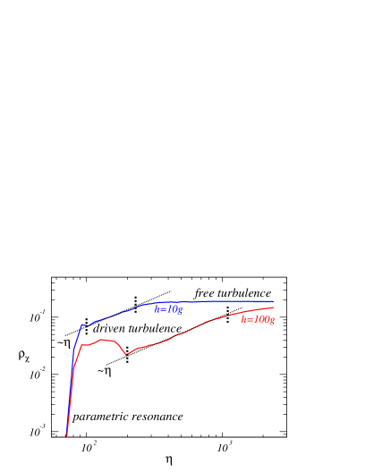
Figure 13: Different phases of evolution of the energy density in the $\chi$ field with conformal time $\eta$ from the initial parametric resonance through driven turbulence and free turbulence (characterised by the end of growth of $\rho_{\chi}$). The model is given by an effective potential $V(\phi,\chi)=\lambda[(1/4)\phi^{4}+(1/2)g\phi^{2}\chi^{2}+(1/4)h\chi^{4}]$. From Ref. MT04 .

Recent work Allahverdi has suggested that if number-violating processes are suppressed relative to number-conserving interactions after preheating then the universe could enter a “quasi-thermal” phase which relaxes to a kinetic equilibrium for some period before number-violating interactions establish full chemical equilibrium. This could occur if the gauge bosons mediating the number-violating process acquire a large mass, suppressing these interactions and further reducing the temperature when full thermal equilibrium is reached.

X.9 Interesting applications of preheating

The nature of preheating lends itself to a number of novel effects which we discuss briefly.

X.9.1 Non-thermal symmetry restoration and phase transitions

It was pointed out by Kofman et al.KLS96 that the growth of fluctuations can lead to non-equilibrium restoration of broken symmetries. Although the notion of an effective potential is not well-defined far from equilibrium the basic ideas are most easily understood using the concept. Consider a typical broken symmetry potential

$$V(\phi,\chi)=\frac{\lambda}{4}(\phi^{2}-v^{2})^{2}+\frac{g^{2}}{2}\phi^{2}\chi^{2}\,.$$ (277)

If $\langle\chi\rangle=0$ then the only minima correspond to $\chi=0;\phi=\pm v$ and the curvature of the potential at $\phi=\chi=0$ is: $V_{\phi\phi}=-\lambda v^{2}<0$. However, if there is parametric resonance then the effective mass of $\phi$ at the point $\phi=0$ is:

$$m_{\phi,{\rm eff}}^{2}=-\lambda v^{2}+3\lambda\langle\delta\phi^{2}\rangle+g^{2}\langle\chi^{2}\rangle\,.$$ (278)

As a result, there is the exciting possibility that the growth of fluctuations can make $m_{\phi,{\rm eff}}^{2}>0$ with the associated possibility of restoring GUT symmetries. When backreaction ends the resonant growth and the subsequent expansion of the universe causes the variances to decay and $m_{\phi,{\rm eff}}^{2}\rightarrow-\lambda v^{2}<0$, breaking the symmetry again.

The danger of this symmetry breaking is the possibility of producing topological defects that inflation was designed to take care of! The non-equilibrium nature of the symmetry restoration makes it difficult to know when defects will be produced and to estimate their density KK97 ; TKKL98 ; RC90 . In general defect densities during non-equilibrium phase transitions are determined by the correlation length of the field at the moment when the relaxation timescale of the inflaton is equal to the time left before the phase transition zurek1 ; zurek2 , rather than the Hubble scale as in the usual Kibble mechanism. Preheating provides a wonderful laboratory for studying non-equilibrium phase transitions with potentially important implications for inflation model building.

X.9.2 Amplification of vector fields

So far we have focused on the amplification of scalar and fermion fields. It is also possible to resonantly amplify vector fields. One of the most interesting cases is the amplification of a $U(1)$ gauge field like electromagnetism with vector potential $A_{\mu}$. The minimal approach is to couple $A_{\mu}$ to a complex scalar field $\sigma$ via the covariant derivative: $D_{\mu}\equiv\nabla_{\mu}+ie\sigma A_{\mu}$, where $e$ is the usual charge. The kinetic term $D_{\mu}\sigma(D^{\mu}\sigma)^{*}$ leads to an effective mass for the “photon” of

$$m_{A}^{2}=2e^{2}|\sigma|^{2}\,,$$ (279)

which breaks the $U(1)$ symmetry when $\sigma$ condenses. The Fourier modes, $A_{k}$, of the spatial part of the vector potential then obey Bassett01b ; FG01 ; RC90

$$A_{k}^{\prime\prime}+(k^{2}+2e^{2}a^{2}|\sigma|^{2})A_{k}=-\sigma_{c}aA_{k}^{\prime}\,,$$ (280)

where ^′ again denotes derivative with respect to conformal time and $\sigma_{c}$ is the electrical conductivity of the medium. Initially during preheating $\sigma_{c}\simeq 0$ and choosing a quartic potential for $\sigma$ implies that this equation becomes formally identical to Eq. (249) and there is exponential growth of $A_{k}$ fluctuations within the appropriate resonance bands.

Applying this elegant mechanism to the generation of the observed large scale magnetic fields of order $10^{-6}{\rm G}$ is complicated by several factors - (1) the $U(1)$ symmetry does not exist in this simple form above the electroweak symmetry energy but is unified with the weak force. Hence one needs to study the full theory. (2) The growth of conductivity that must generically occur during preheating provides a strong damping term to Eq. (280) which means that any predictions are very model dependent and difficult to make. (3) Resonance can only amplify an existing seed field. (4) The coupling to the $\sigma$ field can make the spectrum of $A_{k}$ very red if $e$ is to large. Nevertheless, preheating remains a very promising era for generating large-scale magnetic fields, see e.g., mag1 ; mag2 .

XI The evolution of metric perturbations during reheating

Until now we have neglected metric perturbations in the dynamics of all fields just as we initially neglected backreaction and rescattering. The neglect of metric perturbations is technically incorrect (it violates the Einstein field equations) but is sometimes a good approximation, sometimes not, in the sense that in some cases their inclusion can cause fundamental changes to the dynamics of the fields. A simple example is provided by the ekpyrotic universe. If we neglect metric perturbations, the perturbation in $\varphi$ corresponding to the separation of two branes exhibits a nearly scale-invariant spectrum Khoury01 ; Kallosh01 . The inclusion of metric perturbations leads to a blue-tilted spectrum given by Eq. (166) Wands98 ; Lyth02ekp1 ; Lyth02ekp2 ; Bran01 ; Hwang02eky ; Tsujiekp ; Allen04 .

Another example is provided by a single inflaton, non-minimally coupled to gravity with an interaction $V_{\rm int}(\phi)=(1/2)\xi R\phi^{2}$ with vanishing bare mass of $\phi$. The effective mass of the inflaton is then $m_{{\rm eff}}^{2}=\xi R$. Hence with the appropriate sign of $\xi$ the effective mass squared is negative, the field is tachyonic and we should expect exponential, runaway growth of the fluctuations for all modes satisfying $k^{2}/a^{2}<|\xi|R$, i.e., the very long-wavelength modes. In the absence of metric perturbations this is indeed what happens. The field fluctuations exhibit exponential increase for $k\sim 0$. Note that beyond a critical wavenumber $k_{{\rm crit}}\sim\sqrt{|\xi|Ra^{2}}$ there is no negative instability since the effective mass becomes positive due to the momentum of the modes.

This picture changes completely if we consistently include metric perturbations however BT . The equations of motion for $\delta\phi_{k}$ now are coupled to the linear metric perturbations (e.g. $\Phi$ and $\Psi$ in the longitudinal gauge). Since the field is non-minimally coupled the anisotropic stress does not vanish and $\Phi\neq\Psi$.

However, despite the apparent complexity of the resulting equations they are actually made integrable by the addition of metric perturbations and one can show analytically that the long-wavelength solution ($k\to 0$) is BT

$$\delta\phi=-\frac{\dot{\phi}_{0}(t)}{aF}\left(c_{1}-2c_{2}\int aF{\rm d}t\right)\,,$$ (281)

where $\phi_{0}(t)$ is the homogeneous part of the inflaton, $F\equiv 1-8\pi\xi\phi_{0}^{2}(t)/m_{\rm pl}^{2}$ and $c_{1}$ and $c_{2}$ are integration constants. Equation (281) shows that the long-wavelength modes do not grow at all, in complete contrast to the naive estimate without including metric perturbations. This is not too surprising since there is no relative entropy perturbation for a single field and the intrinsic entropy perturbation is proportional to $k^{2}\Psi_{k}$ so is negligible on large scales. As a result ${\cal R}$ or $\zeta$ is conserved in the $k\to 0$ limit.

The contrast between the results in the two cases is illustrated in Fig. 14 which shows the spectrum of $\delta\phi_{k}$ at the end of reheating for $\xi=-100$ both with and without the inclusion of metric perturbations. The two spectra differ by five orders of magnitude at $k\sim 0$.

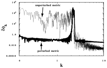
Figure 14: The spectrum of field fluctuations for $\xi=-100$ for both the perturbed and unperturbed metrics in the case of the quartic inflaton potential $V(\phi)=(1/4)\lambda\phi^{4}$ with a non-minimal coupling $(1/2)\xi R\phi^{2}$ BT . When metric perturbations are included, the super-Hubble resonance disappears and is replaced by a single, sub-Hubble band.

This non-minimally coupled inflaton model clearly illustrates that there are cases where neglecting metric perturbations gives a wrong picture of preheating. Our aim here is to discuss when such cases can be expected and what the implications of including metric perturbations is in general, both on large scales and small scales (relevant to black hole formation).

A fundamental question related to preheating is whether it can affect the evolution of super-Hubble metric perturbations. This is crucial since inflationary models are tested against the CMB and hence if reheating affects these predictions it will make model verification and falsification significantly more complex.

XI.1 The criterion for the growth of metric perturbations

After a significant amount of work KH96 ; NT96 ; TN98 ; PE98 ; Bassett99p1 ; Bassett99p2 ; Bassett00p1 ; Bassett00p2 ; Finelli99 ; Finelli00 ; PE98 ; EP99 , it has become clear that in order for preheating to affect super-Hubble metric perturbations there are certain criteria which need to be satisfied Tsuji02 . The most important of these is that there must be an entropy/isocurvature perturbation mode which is not suppressed on very large scales JS00 ; Ivanov00 ; Liddle99 (i.e., that has a power spectrum that it not too blue). When the effective mass of entropy field perturbation $\delta s$ is light relative to the Hubble rate $H$ during inflation, i.e.,

$$\mu_{s}^{2}\equiv V_{ss}+3\dot{\theta}^{2}~{}\mbox{\raisebox{-4.30554pt}{$\stackrel{{\scriptstyle\textstyle<}}{{\textstyle\sim}}$}}~{}H^{2}\,,$$ (282)

$\delta s$ is not suppressed on super-Hubble scales during inflation [See Eq. (183)]. Then during preheating if $\delta s$ is resonantly amplified due to a time-dependent effective mass, this can lead to the growth of ${\cal R}$ on large scales by Eq. (187), thereby altering the power spectrum generated during inflation. In contrast, if the entropy perturbation is heavy during inflation, ($\mu_{s}^{2}\gg H^{2}$) then $|\delta s|\sim a^{-3/2}$ and the growth during preheating means that the change of ${\cal R}$ is negligible before backreaction ends the resonance.

XI.1.1 Quadratic potential

Let us first consider the simple case corresponding to two fields with effective potential:

$$V(\phi,\chi)=\frac{1}{2}m_{\phi}^{2}\phi^{2}+\frac{1}{2}g^{2}\phi^{2}\chi^{2}\,.$$ (283)

Since $|\tan\theta|=|\dot{\chi}/\dot{\phi}|\ll 1$ during inflation, one can estimate the effective mass (282), as

$$\mu_{s}^{2}\simeq V_{\chi\chi}=g^{2}\phi^{2}\,,$$ (284)

where we used Eq. (185). In order for preheating to occur, we require a large resonance parameter, $q_{i}=g^{2}\phi_{i}^{2}/(4m_{\phi}^{2})\gg 1$, at the beginning of reheating, which translates into the condition $g\gg 10^{-5}$ (where we used $\phi_{i}=0.2m_{\rm pl}$ and $m_{\phi}=10^{-6}m_{\rm pl}$). By using the slow-roll approximation, $H^{2}\sim m_{\phi}^{2}\phi^{2}/m_{\rm pl}^{2}$, one can show that the effective mass $\mu_{s}$ is much larger than $H$ during inflation when preheating occurs:

$$\frac{\mu_{s}^{2}}{H^{2}}\sim\left(g\frac{m_{\rm pl}}{m_{\phi}}\right)^{2}\gg 1\,.$$ (285)

Hence the long-wavelength modes of $\delta s$ are exponentially suppressed during inflation and the entropy perturbation has a highly blue tilted spectrum. To see this note that for $k\sim 0$ $\delta s\simeq a^{-3/2}$ while for the perturbations deep inside the Hubble radius ($k\gg aH$), the modes evolve as in the vacuum state in Minkowski spacetime. Hence the long-wavelengths suffer suppression while the short wavelengths do not, leading to a blue spectrum. Even if $\delta s$ is amplified by a factor $10^{5}$-$10^{6}$ during preheating, the suppression of the entropy perturbation in the preceding inflationary stage is too strong to give rise to the variation of curvature perturbations on super-Hubble scales by the time backreaction ends the resonance due to the growth of sub-Hubble scale fluctuations. As a result the existence of the preheating stage does not affect the CMB power spectrum for the model given by Eq. (283).

XI.1.2 Quartic potential

One elegant case in which the entropy field perturbation is not necessarily suppressed is the conformal model with potential

$$V(\phi,\chi)=\frac{1}{4}\lambda\phi^{4}+\frac{1}{2}g^{2}\phi^{2}\chi^{2}\,.$$ (286)

In the linear regime of preheating where $|\chi|\ll|\phi|$ is satisfied, one has $|\theta|\ll 1$ and $V_{ss}\simeq V_{\chi\chi}=g^{2}\phi^{2}$ in Eq. (183). Then Eq. (183) approximately reads

$$\frac{{\rm d}^{2}}{{\rm d}x^{2}}\delta\tilde{s}+\left[\kappa^{2}+\frac{g^{2}}{\lambda}{\rm cn}^{2}\left(x;\frac{1}{\sqrt{2}}\right)\right]\delta\tilde{s}=0\,,$$ (287)

where $\delta\tilde{s}\equiv a\delta s$, $x$ and $\kappa^{2}$ are defined in the same way as in Eq. (249). Here we used the solution (248) and also neglected the terms which include $\dot{\theta}$. We find that Eq. (286) is the same equation as the one that the perturbation $\delta\chi$ obeys. Hence we can use the stability-instability chart of Lamé equation for $\delta\tilde{s}$ at the linear regime of preheating. When the field $\chi$ grows comparable to $\phi$, the field trajectory becomes curved ($\dot{\theta}\neq 0$) with $\theta$ of order 1. Then the approximate equation (287) can no longer be used at this stage.

As we already explained in the previous section, the long wavelength modes of the perturbation $\delta s$ are amplified for the parameter range $n(2n-1)<g^{2}/\lambda<n(2n+1)$ with integer $n$. While $\delta s$ is exponentially suppressed during inflation for $g^{2}/\lambda\gg 1$, this suppression does not occur for $g^{2}/\lambda\sim 1$ because of the light effective mass Bassett00p1 ; Finelli00 .

Since the super-Hubble modes of $\delta s$ grow exponentially during preheating, we can expect that large-scale curvature perturbations may be enhanced for the parameter range around $g^{2}/\lambda\sim 2$.

Numerical simulations based upon the Hartree approximation shows that this actually happens for $g^{2}/\lambda\sim 2$ around the end of preheating once the entropy field fluctuation is sufficiently amplified Zibin00 ; Tsuji00 , see Fig. 15. However large-scale curvature perturbations do not exhibit parametric amplification for $g^{2}/\lambda\gtrsim 8$ due to the suppression during inflation within the mean-field approximation Zibin00 . If we take into account a negative non-minimal coupling $(1/2)\xi R\chi^{2}$, curvature perturbations can grow even for $g^{2}/\lambda\sim 50$ Tsuji02 .

Is the amplification of large-scale metric perturbations consistent with causality? The resolution of this is that there is no transfer of energy over super-Hubble scales. Instead, the pre-existing entropy perturbation (which for $g^{2}/\lambda<{\cal O}(1)$ is light) is amplified by the resonance. The power of isocurvature perturbations to alter super-Hubble adiabatic perturbations is well known Bassett99p2 . The large-scale entropy perturbations do drive variation in ${\cal R}$ and there is no violation of causality.

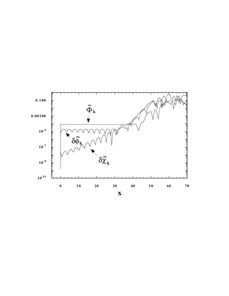
Figure 15: Evolution of the gravitational potential $\tilde{\Phi}_{k}\equiv k^{3/2}\Phi_{k}$ together with the field perturbations $\delta\tilde{\chi}_{k}\equiv k^{3/2}{\chi}_{k}/m_{\rm pl}$, and $\delta\tilde{\phi}_{k}\equiv k^{3/2}{\phi}_{k}/m_{\rm pl}$ on cosmological scales during inflation and preheating for $g^{2}/\lambda=2$. With the use of the Hartree approximation we find that super-Hubble metric perturbations are amplified during preheating.

When the entropy perturbations are sufficiently enhanced, one can expect that the correlation between adiabatic and isocurvature should be very strong. This should alter the shape of the CMB power spectrum as we already have seen in Sec. VIII (see Fig. 8). It provides a proof that reheating can affect the predictions of the model.

It is certainly of interest to see whether or not the parameter region $g^{2}/\lambda\sim 2$ is compatible with the CMB constraints. This requires a full numerical study of non-linear perturbation dynamics which includes the decay of scalar fields. Another interesting model which leads to the enhancement of curvature perturbations is the hybrid (double) inflation model with a tachyonic instability Tsuji02 . However almost all other two-field models have cosmological predictions that are not violently affected by the details of preheating.

XI.2 Production of particles and magnetic fields through metric perturbations

The growth of metric perturbation during preheating means that on certain scales the assumption of FRW metric is bad. Including the metric perturbations one now has a background with no symmetries and non-vanishing Weyl tensor, which as a result is not conformally flat. All the standard results about conformally invariant fields no longer hold.

A simple example is provided by massless fermion fields. In a flat FRW background there is no production due to the expansion of the universe since the equation of motion can be brought into Minkowski form by suitable rescaling. However, in the presence of metric perturbations we can treat fermions in an external field given by the metric perturbations CV90 ; CV92 ; Frieman89 , and hence there will be particle production because of this external field. In the massless case, a direct computation BT10 shows that in the massless limit the number of particles produced is:

$$N_{T}=\frac{1}{160\pi a^{3}}\int\frac{{\rm d}^{4}p}{(2\pi)^{4}}\theta(p^{0})\theta(p^{2})|\tilde{C}^{abcd}(p)|^{2}\,,$$ (288)

where $p$ denotes four-momentum, $\theta$ is the Heaviside step function and $\tilde{C}^{abcd}$ is the Fourier transform of the Weyl tensor:

$$\tilde{C}^{abcd}(p)\equiv\int{\rm d}^{4}xe^{ip_{\mu}x^{\mu}}C^{abcd}\,,$$ (289)

which is the trace-free part of the full Riemann tensor. In conformally flat spacetimes $C^{abcd}=0$, but when we include metric perturbations the Weyl tensor does not vanish but depends linearly on the metric perturbations BT10 . As a general rule, the number of particle produced as a result of the breaking of conformal flatness is therefore small, being quadratic in the metric perturbations. However, in preheating, with the enhancement of metric fluctuations in certain wavelengths the production can be significant. In Ref. BT10 it was shown that this metric perturbation-driven production of fermions dominates the homogeneous production of fermions in the standard chaotic inflation model with the quartic potential for fermion masses below $10^{5}\,{\rm GeV}$ BT10 .

A similar discussion can be made for Maxwell fields whose equation of motion is conformally invariant. The observed large-scale, large-amplitude magnetic fields are therefore somewhat of a mystery since they are not amplified by the expansion of the universe. Allowing for the perturbative breaking of conformal flatness of FRW by metric perturbations offers a generic and viable mechanism for the generation of magnetic fields during inflation Bassett00p2 ; Maroto01 ; Bassett01b ; MMNR05 .

XI.3 Primordial black hole formation during preheating

Although we have shown that typically (at least in two-field models) large wavelength fluctuations do not cause a large change in ${\cal R}$ or $\zeta$ except for certain cases, and hence do not usually affect the predictions of inflation for the CMB, preheating can lead to the growth of metric fluctuations on smaller scales, around the Hubble scale, $k=aH$ which is many orders of magnitude smaller than CMB-relevant modes at preheating. As a result one might expect that preheating may lead to copious over-production of primordial black holes (PBH) GM00 ; Bassett01a ; FK01 ; FK02 .

The PBH density can be constrained in a number of ways. When they evaporate via Hawking radiation they release entropy and high-energy products that, depending on when they evaporate, can destroy the predictions of nucleosynthesis or predict $\gamma$-ray flux in excess of that observed today. PBH can also simply overclose the universe since their energy density scales as $a^{-3}$ compared with the radiation scaling law of $a^{-4}$.

However, there are several robust reasons to believe that resonant preheating does not significantly alter the abundance of PBH’s. First, the peak in the power spectrum of density perturbations (the relevant quantity for PBH production), is always at sub-Hubble wavelengths since the maximum momentum amplified is

$$\frac{k_{{\rm max}}}{H}\sim\frac{m_{\rm pl}}{\phi}q^{1/4}\gg 1\,,$$ (290)

where the final inequality follows from requiring strong preheating $q\gg 1$ and noting that $\phi<m_{\rm pl}$ at the start of preheating in all known inflationary models. Three dimensional lattice simulations PBHkyoto using a modified version of LATTICEEASY latticeeasy show that the peak value of the density perturbation satisfies $\delta_{H}<1$, and occurs at scales significantly smaller than the Hubble scale which is relevant to PBH production. Since the resulting density power spectrum is typically $\propto k^{3}$ on these scales PBHkyoto the value of $\delta_{H}\sim 10^{-4}$ is typical at the Hubble scale, implying no excess PBH production.

In the case of tachyonic preheating, long-wavelength modes are amplified during the tachyonic (spinodal) phase. In these cases the peak of the spectrum can be at scales close to the Hubble scale and approach the threshold for over-production of PBH PBHkyoto2 . Nevertheless, all simulations to date have been limited by numerical resolution (in three dimensions) and have not consistently included metric perturbations or have not covered all the relevant length scales of the problem.

XII Curvaton

The original inflation models assumed that the field that drives inflation is also the field responsible for the origin of structure in our Universe. This seems an economical approach, but recently several authors have begun to reconsider whether this is necessarily so. Might it be possible that perturbations in some field other than the inflaton could be responsible for the primordial density perturbation? If so, we need to interpret observational constraints upon the dynamics of inflation quite differently.

Consider a weakly-coupled, massive scalar field, $\chi$, that decays some time after inflation has ended. There are many such scalar degrees of freedom in supersymmetric theories and if they are too weakly coupled, and their lifetime is too long, this may lead to the moduli or Polonyi problem. Assuming the field is displaced from the minimum of its effective potential at the end of inflation, the field evolves little until the Hubble rate drops below its effective mass. Then it oscillates, with a time-averaged equation of state for a pressureless fluid, $P_{\chi}=0$, (or, equivalently, a collection of non-relativistic particles). It would eventually come to dominate the energy density of the Universe, so to avoid disrupting the successful “hot big bang” model of the early universe and, in particular, to preserve the successful radiation-dominated model of primordial nucleosynthesis, we require that such fields decay into radiation before $t\sim 1$ second. For a weakly-coupled field that decays with only gravitational strength, $\Gamma\sim m_{\chi}^{3}/m_{\rm pl}^{2}$, this requires $m_{\chi}>100$ TeV. Indeed such late-decaying scalar fields may be no bad thing. Late-entropy production reduces the minimum duration of inflation required to produce the total entropy of our observed universe and dilutes other dangerous relics such as gravitinos, primordial black holes or monopoles.

But there is a further important feature of late-decaying scalar fields that has only recently received serious consideration. If the field is inhomogeneous then it could lead to an inhomogeneous radiation density after it decays Mollerach90 ; LindeMukhanov96 . This is the basis of the curvaton scenario Enqvist02 ; Lyth02 ; Moroi01 .

If the curvaton field is light ($m<H$) during inflation then small-scale quantum fluctuations will lead to a spectrum of large-scale perturbations, whose initial amplitude at Hubble-exit is given by Eq. (196). When the Hubble rate drops and the field begins oscillating after inflation, this leads to a primordial density perturbation in the $\chi$-field:

$$\zeta_{\chi}=-\psi+\frac{\delta\rho_{\chi}}{3\rho_{\chi}}\,,$$ (291)

where $\rho_{\chi}=m_{\chi}^{2}\chi^{2}/2$. $\zeta_{\chi}$ remains constant for the oscillating curvaton field on large scales, so long as we can neglect its energy-transfer, i.e., before it decays. Using Eq. (196) for the field fluctuations at Hubble-exit and neglecting any non-linear evolution of the $\chi$-field after inflation (consistent with our assumption that the field is weakly coupled), we have

$${\cal P}_{\zeta_{\chi}}\simeq\left(\frac{H}{6\pi\chi}\right)^{2}_{k=aH}\,.$$ (292)

The total density perturbation (82), considering radiation, $\gamma$, and the curvaton, $\chi$, is given by

$$\zeta=\frac{4\rho_{\gamma}\zeta_{\gamma}+3\rho_{\chi}\zeta_{\chi}}{4\rho_{\gamma}+3\rho_{\chi}}\,.$$ (293)

Thus if the radiation generated by the decay of the inflaton at the end of inflation is unperturbed (${\cal P}_{\zeta_{\gamma}}^{1/2}\ll 10^{-5}$) the total curvature perturbation grows as the density of the $\chi$-field grows relative to the radiation: $\zeta\sim\Omega_{\chi}\zeta_{\chi}$.

Ultimately the $\chi$-field must decay (when $H\sim\Gamma$) and transfer its energy density and, crucially, its perturbation to the radiation and/or other matter fields. In the simplest case that the non-relativistic $\chi$-field decays directly to radiation a full analysis Malik02 ; Gupta of the coupled evolution equation gives the primordial radiation perturbation (after the decay)

$$\zeta_{\gamma}=r(p)\zeta_{\chi}\,,$$ (294)

where $p\equiv[\Omega_{\chi}/(\Gamma/H)^{1/2}]_{\rm initial}$ is a dimensionless parameter which determines the maximum value of $\Omega_{\chi}$ before it decays, and empirically we find Gupta

$$r(p)\simeq 1-\left(1+\frac{0.924}{1.24}p\right)^{-1.24}\,.$$ (295)

For $p\gg 1$ the $\chi$-field dominates the total energy density before it decays and $r\sim 1$, while for $p\ll 1$ we have $r\sim 0.924p\ll 1$.

Finally combining Eqs. (292) and (294) we have

$${\cal P}_{\zeta_{\gamma}}\simeq r^{\,2}(p)\left(\frac{H}{6\pi\chi}\right)^{2}_{k=aH}\,.$$ (296)

In contrast to the inflaton scenario the final density perturbation in the curvaton scenario is a very much dependent upon the physics after the field perturbation was generated during inflation. For instance, if the curvaton lifetime is too short then it will decay before it can significantly perturb the total energy density and ${\cal P}_{\zeta_{\gamma}}^{1/2}\ll 10^{-5}$. The observational constraint on the amplitude of the primordial perturbations gives a single constraint upon both the initial fluctuations during inflation and the post-inflationary decay time. This is in contrast to the inflaton scenario where the primordial perturbation gives a direct window onto the dynamics of inflation, independently of the physics at lower energies. In the curvaton scenario there is the possibility of connecting the generation of primordial perturbations to other aspects of cosmological physics. For instance, it may be possible to identify the curvaton with fields whose late-decay is responsible for the origin of the baryon asymmetry in the universe, in particular with sneutrino models of leptogenesis (in which an initial lepton asymmetry is converted into a baryon asymmetry at the electroweak transition) sneutrino .

The curvaton scenario has re-invigorated attempts to embed models of inflation in the very early universe within minimal supersymmetric models of particle physics constrained by experiment Enqvist03cur ; mssm ; EKM03 ; Postma02 ; Postma03 ; Hamaguchi03 ; Dimo03 ; McDonald03 . It may be possible that the inflaton field driving inflation can be completely decoupled from visible matter if the dominant radiation in the universe today comes from the curvaton decay rather than reheating at the end of inflation. Indeed the universe need not be radiation-dominated at all until the curvaton decays if instead the inflaton fast-rolls at the end of inflation.

The curvaton offers a new range of theoretical possibilities, but ultimately we will require observational and/or experimental predictions to decide whether the curvaton or inflaton generated the primordial perturbation.

XII.1 Non-Gaussianity

The best way to distinguish between different scenarios for the origin of structure could be the statistical properties of the primordial density perturbation. All the inflationary models we have discussed start with small-scale vacuum fluctuations of an effectively free scalar field, described by a Gaussian random field, with vanishing three-point function. Deviations from Gaussianity in the curvaton scenario can be parameterised by a dimensionless parameter $f_{nl}$ Komatsu03 defined in Eq. (94). In terms of the initial curvaton density perturbation (291) on spatially-flat hypersurfaces we have, from Eq. (294),

$$\zeta_{\gamma}=\frac{r}{3}\left(\frac{\delta\rho_{\chi}}{\rho_{\chi}}\right)_{\psi=0}\,.$$ (297)

When the curvaton field begins oscillating about a quadratic minimum of its potential we have $\rho_{\chi}=m_{\chi}^{2}\chi^{2}/2$, and thus, in terms of the Newtonian potential on large scales in the matter-dominated era, $\Phi=-3\zeta/5$, this gives

$$\Phi=-\frac{r}{5}\left(\frac{2\chi\delta\chi+\delta\chi^{2}}{\chi^{2}}\right)\,.$$ (298)

Identifying $\Phi_{\rm Gauss}=-(2r/5)\delta\chi/\chi$ and substituting into (94) we obtain Lyth03

$$f_{nl}=-\frac{5}{4r}\,.$$ (299)

In other words, the smaller the fraction of the radiation density due to curvaton decay, the larger the non-Gaussianity of the primordial density perturbation. Eq. (299) corrects a sign error in the expression for $f_{NL}$ given in Ref. Lyth03 . We note that $f_{nl}$ is subject to a modification when gravitational second-order corrections are taken into account, but it reproduces Eq. (299) in the limit $r\ll 1$ Bartolo04cur .

Current bounds from the WMAP satellite require $-58<f_{nl}<134$ at the 95% confidence limit Komatsu03 , and hence require $r>0.021$ but future experiments such as Planck could detect $f_{nl}$ as small as around $5$.

By contrast in the inflaton scenario the inflaton field fluctuations at horizon-crossing determine the large-scale curvature perturbation $\zeta$ which will remain constant on super-Hubble scales. One can estimate the amplitude of the three-point correlation function by noting that the local amplitude of fluctuations will depend on local variations in the Hubble rate. This gives a robust estimate of the primordial non-Gaussianity in the inflaton scenario Maldacena02

$$f_{nl}\sim\frac{n_{s}-1}{4}\,,$$ (300)

where $n_{s}-1$ is the scale-dependence of the primordial power spectrum. Note that this estimate relies on the adiabaticity of the perturbations in the inflaton scenario which ensures that there exists a non-linearly conserved density perturbation on large scales, from Hubble-exit during inflation until last-scattering of the CMB photons. Any detection of primordial non-Gaussianity $f_{nl}>1$ would therefore rule out this inflaton scenario.

XII.2 Residual isocurvature perturbations

In multi-field scenarios such as the curvaton scenario the initial perturbation is supposed to be a non-adiabatic perturbation and hence can in principle leave behind a residual non-adiabatic component. In the curvaton scenario, perturbations in just one field, the curvaton, would be responsible for both the total primordial density perturbation and any isocurvature mode and hence there is the clear prediction that the two should be completely correlated, corresponding to $\cos\Delta=\pm 1$ in Eq. (205), or $A_{r}/A_{s}\to 0$ in Eq. (221) and $n_{2}=n_{3}=n_{c}$.

Using $\zeta_{i}$ for different matter components it is easy to see how the curvaton could leave residual isocurvature perturbations after the curvaton decays. If any fluid has decoupled before the curvaton contributes significantly to the total energy density that fluid remains unperturbed with $\zeta_{i}\simeq 0$, whereas after the curvaton decays the photons perturbation is given by (296). Thus a residual isocurvature perturbation (83) is left

$$S_{i}=-3\zeta_{\gamma}\,,$$ (301)

which remains constant for decoupled perfect fluids on large scales.

The observational bound on isocurvature matter perturbations completely correlated with the photon perturbation, is Gordon02

$$-0.53<\frac{S_{B}+(\rho_{\rm c}/\rho_{B})S_{\rm c}}{\zeta_{\gamma}}<0.43\,.$$ (302)

In particular if the baryon asymmetry is generated while the total density perturbation is still negligible then the residual baryon isocurvature perturbation, $S_{B}=-3\zeta_{\gamma}$ would be much larger than the observational bound and such models are thus ruled out. The observational bound on CDM isocurvature perturbations are stronger by the factor $\rho_{\rm c}/\rho_{B}$ although CDM is usually assumed to decouple relatively late.

An interesting amplitude of residual isocurvature perturbations might be realised if the decay of the curvaton itself is the non-equilibrium event that generates the baryon asymmetry. In this case the net baryon number density directly inherits the perturbation $\zeta_{B}=\zeta_{\chi}$ while the photon perturbation $\zeta_{\gamma}\leq\zeta_{\chi}$ may be diluted by pre-existing radiation and is given by Eq. (294). Note that so long as the net baryon number is locally conserved it defines a conserved perturbation on large scales, even though it may still be interacting with other fluids and fields. Hence the primordial baryon isocurvature perturbation (83) in this case is given by

$$S_{B}=3(1-r)\zeta_{\chi}=\frac{3(1-r)}{r}\zeta_{\gamma}\,.$$ (303)

But there is no lower bound on the predicted amplitude of residual non-adiabatic modes and the non-detection of primordial isocurvature density perturbations cannot be used to rule out all alternative scenarios. For instance if after the curvaton decays at sufficiently high temperature and all the particles produced relax to an thermal equilibrium abundance, characterised by a common temperature and vanishing chemical potential then no residual isocurvature perturbations survive. In this case there is a unique attractor trajectory in phase-space and only adiabatic perturbations (along this trajectory) survive on large scales.

XIII Modulated reheating

The curvaton scenario is one possible way in which a light scalar field during inflation can influence the primordial density perturbation on large scales after inflation. An alternative possibility Dvali03_1 ; Kofman03 is that the primordial perturbation could be generated by the spatial variation of the inflaton decay rate, $\Gamma$, at the end of inflation.

The decay rate of the inflaton $\phi$ in the “old” reheating scenario is given by $\Gamma\sim\lambda^{2}m$, where $m$ is the inflaton mass and $\lambda$ a dimensionless coupling of the inflaton to other light fields. When $\Gamma$ is less than the Hubble rate at the end of inflation, the reheating temperature $T_{{\rm rh}}$ is estimated as

$$T_{{\rm rh}}\sim\sqrt{\Gamma m_{\rm pl}}\sim\lambda\sqrt{mm_{\rm pl}}\,.$$ (304)

If the local coupling strength $\lambda$ is dependent on the local value of another scalar field, $\chi$, this can give rise to fluctuations in the reheating temperature:

$$\frac{\delta T_{{\rm rh}}}{T_{{\rm rh}}}\sim\frac{\delta\Gamma}{\Gamma}\sim\frac{\delta\lambda}{\lambda}\,.$$ (305)

Thus density perturbations after inflation are sourced by local fluctuations in $\chi$. If $\chi$ is light during inflation then it can acquire an almost scale-invariant spectrum of perturbations at Hubble exit, which are then imprinted on the radiation field during reheating. It is natural to consider perturbed couplings, since the coupling “constants” of the low-energy effective action in string theory are generally functions of the vacuum expectation values of light moduli fields Kofman03 . In what follows we refer to this scenario as “modulated reheating”.

Let us estimate the curvature perturbation in the radiation fluid generated after inflation in the modulated reheating scenario. In doing so we recall that the curvature perturbation $\zeta$, defined in Eq. (52), can be interpreted as the dimensionless density perturbation on spatially flat hypersurfaces, which are separated by a uniform expansion. In a region with a larger local decay rate, $\Gamma+\delta\Gamma$, the local energy density on spatially flat hypersurfaces differs with respect to the average by an amount $\delta\rho=H\rho\delta t$ due to the earlier change from matter to radiation equation of state. Since the average decay time is given by $t=\Gamma^{-1}$, the perturbation of the local decay rate corresponds to the perturbed decay time $t+\delta t$ with $\delta t=-\delta\Gamma/\Gamma^{2}$. Then by using Eq. (81), the curvature perturbation in radiation fluid after the decay of inflaton is found to be

$$\zeta_{\gamma}=\frac{1}{4}\left(\frac{\delta\rho}{\rho}\right)_{\psi=0}=-\frac{1}{4}\frac{H\delta\Gamma}{\Gamma^{2}}=-\frac{1}{6}\frac{\delta\Gamma}{\Gamma}\,,$$ (306)

where in the last equality we used $t=(2/3)H^{-1}=\Gamma^{-1}$ at the decay time.

The validity of this estimate, which assumes a sudden decay of the inflaton, can be investigated numerically using the coupled evolution equations for perturbations with interacting fluids Malik04 . Here we treat the inflaton is treated as a pressureless fluid decaying to a radiation fluid with a perturbed decay rate Mazumdar03_2 ; Mata03 ; Ver03 . The background energy density of the inflaton field $\rho_{\phi}$ and radiation $\rho_{\gamma}$ satisfy

$$\dot{\rho}_{\phi} = -3H\rho_{\phi}+Q_{\phi}\,,$$ (307)

$$\dot{\rho}_{\gamma} = -4H\rho_{\gamma}+Q_{\gamma}\,.$$ (308)

Here the energy transfer from inflaton to radiation is characterized by $Q_{\phi}=-\Gamma\rho_{\phi}$ and $Q_{\gamma}=\Gamma\rho_{\phi}$. Introducing dimensionless quantities

$$\Omega_{\phi}\equiv\frac{\rho_{\phi}}{\rho_{\phi}+\rho_{\gamma}}\,,~{}~{}\Omega_{\gamma}\equiv\frac{\rho_{\gamma}}{\rho_{\phi}+\rho_{\gamma}}\,,~{}~{}g\equiv\frac{\Gamma}{H}\,,$$ (309)

the background equations (307) and (308) may be rewritten as

$$\frac{{\rm d}\Omega_{\phi}}{{\rm d}N}=\Omega_{\phi}(1-\Omega_{\phi}-g)\,,$$ (310)

$$\frac{{\rm d}g}{{\rm d}N}=\frac{g}{2}(4-\Omega_{\phi})+\frac{g}{\Gamma}\frac{{\rm d}\Gamma}{{\rm d}N}\,,$$ (311)

with $N$ is the number of e-foldings and $\Omega_{\phi}+\Omega_{\gamma}=1$. We assume that the scalar field whose local expectation value leads to the spatial variation of the decay rate $\Gamma$, makes a negligible contribution to the energy density.

The perturbed energy transfer is given by $\delta Q_{\phi}=-\Gamma\delta\rho_{\phi}-\delta\Gamma\rho_{\phi}$ and $\delta Q_{\gamma}=\Gamma\delta\rho_{\phi}+\delta\Gamma\rho_{\phi}$. The perturbation equations on wavelengths larger than the Hubble radius are Malik02 ; Mata03

$$\dot{\delta\rho}_{i}+3H(\delta\rho_{i}+\delta P_{i})-3(\rho_{i}+P_{i})\dot{\psi}$$

$$=Q_{i}A+\delta Q_{i}\,,$$ (312)

where $i=\phi,\gamma$ for inflaton and radiation.

The gauge-invariant curvature perturbation for each component ($i=\phi,\gamma$) are defined by Eq. (81). Then the total curvature perturbation, $\zeta$, is given by

$$\zeta = \frac{\dot{\rho}_{\phi}}{\dot{\rho}}\zeta_{\phi}+\frac{\dot{\rho}_{\gamma}}{\dot{\rho}}\zeta_{\gamma}\,,$$ (313)

$$= f\zeta_{\phi}+(1-f)\zeta_{\gamma}\,,$$ (314)

where

$$f\equiv\frac{(3+g)\Omega_{\phi}}{(4-\Omega_{\phi})}\,.$$ (315)

Note that this corrects Eq. (2.38) of Ref. Mata03 .

We define a relative entropy perturbation (83) as

$${\cal S}_{\phi\gamma}\equiv 3(\zeta_{\phi}-\zeta_{\gamma})\,,$$ (316)

which leads to a non-adiabatic pressure perturbation (49). Then we find that the evolution equations for $\zeta_{\phi}$ and $\zeta_{\gamma}$ are Mata03

$$\dot{\zeta}_{\phi} = -\frac{\Gamma}{6}\frac{\rho_{\phi}}{\rho}\frac{\dot{\rho}_{\gamma}}{\dot{\rho}_{\phi}}{\cal S}_{\phi\gamma}+H\frac{\rho_{\phi}}{\dot{\rho}_{\phi}}\delta\Gamma_{\phi}^{\rm GI}\,,$$ (317)

$$\dot{\zeta}_{\gamma} = \frac{\Gamma}{3}\frac{\dot{\rho}_{\phi}}{\dot{\rho}_{\gamma}}\left(1-\frac{\rho_{\phi}}{2\rho}\right){\cal S}_{\phi\gamma}-H\frac{\rho_{\phi}}{\dot{\rho}_{\gamma}}\delta\Gamma_{\gamma}^{\rm GI}\,,$$ (318)

where the gauge-invariant perturbation $\delta\Gamma_{i}^{\rm GI}$ is defined by

$$\delta\Gamma_{i}^{\rm GI}=\delta\Gamma-\dot{\Gamma}\frac{\delta\rho_{i}}{\dot{\rho}_{i}}\,.$$ (319)

This describes a non-adiabatic energy transfer Malik04 which can source the entropy perturbation ${\cal S}_{\phi\gamma}$. We include any time variation of the background decay rate $\dot{\Gamma}$ in order to construct the gauge-invariant energy transfer.

Eqs. (317) and (318) show that the presence of the entropy perturbation ${\cal S}_{\phi\gamma}$ and the gauge-invariant perturbation $\delta\Gamma_{i}^{\rm GI}$ leads to the variation of $\zeta_{\phi}$ and $\zeta_{\gamma}$. In what follows we shall consider a situation in which the time variation of $\Gamma$ is neglected. Then by using Eq. (313) together with Eqs. (317) and (318), we find Mazumdar03_2

$$\frac{{\rm d}\zeta}{{\rm d}N} = -\frac{(3+f)\Omega_{\phi}}{4-\Omega_{\phi}}(\zeta-\zeta_{\phi})\,,$$ (320)

$$\frac{{\rm d}\zeta_{\phi}}{{\rm d}N} = \frac{(4-\Omega_{\phi})f}{2(3+f)}(\zeta-\zeta_{\phi})-\frac{f}{3+f}\frac{\delta\Gamma}{\Gamma}\,.$$ (321)

We numerically solve the perturbation equations (320) and (321) together with the background equations (310) and (311), see Fig. 16. Under the initial conditions $\zeta(0)=0.0$, $\zeta_{\phi}(0)=0.0$, $\Omega_{\phi}(0)=0.99$ and $g(0)=0.01$, we find that both $\zeta$ and $\zeta_{\gamma}$ approach the analytic value given by Eq. (306) at late times. As long as $|\zeta_{\phi}(0)|\lesssim 10^{-3}\delta\Gamma/\Gamma$, the evolution of $\zeta$ is similar to the one shown in Fig. 16. When $|\zeta_{\phi}(0)|\gtrsim 10^{-3}\delta\Gamma/\Gamma$, the final value of $\zeta$ exhibits some deviation from the analytic value (306) Mazumdar03_2 . For example one has $\zeta=-0.118\delta\Gamma/\Gamma$ for $\zeta_{\phi}(0)=0.05\delta\Gamma/\Gamma$.

Thus the final curvature perturbation is generated by the perturbed coupling in addition to any initial inflaton fluctuation. In Ref. Tsuji03per the spectra of primordial perturbations were evaluated numerically for the system in which perturbations of both the inflaton and the decay rate coexist. It was shown that even in low energy-scale inflation a nearly scale-invariant spectra, with an overall amplitude set by observations, can be obtained through the conversion of $\chi$ fluctuations into adiabatic density perturbations. A model for fluctuating inflaton coupling was proposed in Ref. Mazumda03_1 using (s)neutrinos as a source for adiabatic perturbations. In Ref. Ackerman04 the generation of density perturbations in preheating was studied for the model in which the coupling $g$ between inflaton and decay products is perturbed by another scalar field. In Ref. BKU modulated fluctuations from hybrid inflation was studied in the case where $\lambda$ and $g$ in Eq. (32) depend upon a light scalar field. It was shown in Ref. BGS05 that if heavy particles are in thermal equilibrium until they become relativistic, perturbations in the annihilation cross section of this particle receive additional sources of fluctuations.

Finally we note that an alternative mechanism combining features of both modulated reheating and the curvaton scenario could arise if after inflation and homogeneous reheating the universe becomes dominated by an oscillating (curvaton-type) field. Primordial perturbations are produced if the decay-rate and/or mass of this curvaton-type field varies Dvali03_2 , even if the curvaton itself has no perturbations, due to spatial variations in the VEV of another light field, $\phi$. Vernizzi Ver03 studied the coupled perturbation equations in this three fluid case finding the resulting primordial perturbation is given by

$$\zeta=r(p)\left[-\frac{4}{3}\frac{\delta M}{M}-\frac{1}{6}\frac{\delta\Gamma}{\Gamma}\right]\,,$$ (322)

where $r(p)$ for the curvaton-type field is given in Eq. (295).

The non-Gaussianity of primordial perturbations in the modulated reheating scenarios was studied in Refs. Ver03 ; Za03 . Unlike the curvaton scenario there is an additional parameter $\alpha_{\Gamma}$ in the model-dependent transfer coefficient

$$\zeta=r\alpha_{\Gamma}\zeta_{\chi}\,.$$ (323)

A simple estimation of the parameter $f_{nl}$ defined in Eq. (95) gives Ver03

$$f_{nl}=-\frac{5}{6r\alpha_{\Gamma}}\,.$$ (324)

The curvaton scenario corresponds to $\alpha_{\Gamma}=-2/3$, see Eq. (299). When the field $\phi$ completely dominates the universe before it decays, one has $r=1$ and $\alpha_{\Gamma}=1/6$ in the modulated reheating scenario, thus giving $f_{nl}=-5$. Hence this scenario has a possibility to confront with the future observations of Planck satellite whose sensitivity should reach to the level $|f_{nl}|\sim 5$.

Figure 16: The evolution of $\zeta$, $\zeta_{\phi}$ and $\zeta_{\gamma}$ (normalized by $\delta\Gamma/\Gamma$) in the modulated reheating scenario with initial conditions $\Omega_{\phi}(0)=0.99$, $\Omega_{\gamma}(0)=0.01$, $g=0.01$, $\zeta(0)=0.0$ and $\zeta_{\phi}(0)=0.0$.

XIV Conclusions

The building of realistic inflationary models will inevitably imply a phase in which multiple fields are studied. Whether we are close to building “realistic” models of inflation is not clear. At present single field models are still the best fit to the data precisely because of their simplicity and lack of free parameters.

As with the search for dark energy dynamics, one of the major challenges for observational cosmology is the hunt for a signature of dynamics. At present all observations are consistent with an exactly scale-invariant Harrison-Zel’dovich primordial spectrum and a universe which today is dominated by a pure cosmological constant. We await conclusive evidence that the Universe is, or ever was dominated by one or more light scalar fields. If such evidence arrives, it will require model-building in ernest.

In science there is a natural resonance between data and theory which drives the complexity of models to roughly match the amount and quality of data available to test them. Until now there has been little motivation - beyond exploring the range of what is possible - for considering models of inflation with many fields which are light compared with the Hubble constant. Entering the era of data-driven cosmology this situation is changing rapidly and although single field models are still arguably the best fits to current CMB and large scale structure data, their dominance must be challenged by making accurate and detailed predictions for models with more than one light field.

Beyond this practical motivation to study multi-field models there is a deep conceptual reason: in single field models the cosmological predictions of inflation are robust and depend very little on the dynamics of reheating. When there are more than one light field this is no longer the case and the full details of reheating and post-inflation dynamics must be considered when comparing the model to the data. On the one hand this opens up the exciting possibility that we may be able to probe details of particle physics beyond the standard model with cosmology while on the other hand it introduces much larger parameter spaces and removes some of the elegant model-independence of single-field inflation.

What experimental progress can we expect in the next decade or two? The Planck satellite should fix $\Omega_{m}h^{2}$ to high precision which, combined with polarisation measurements will help significantly in constraining multi-field inflationary models. Upcoming large galaxy surveys such as those with WFMOS/KAOS, LSST, DES and PANSTARRS will help pin down the matter power spectrum with exquisite accuracy, culminating in the Square Kilometre Array which will find redshifts of around one billion galaxies, giving the ultimate measurement of the power spectrum at $z<1$.

By that time we should have an excellent understanding of galaxy and matter biasing and will be able to study the time-evolution of the power spectrum. Leveraging the CMB and the matter power spectrum (together with traditional distance measurements via type Ia supernovae and baryon acoustic oscillations) should allow us to distinguish between the effects of dark energy (late time evolution) and the effects associated with multi-field inflation. Hopefully we will find that the cosmos exhibits some of the interesting possibilities offered by the dynamics of multiple field inflation.

- (1) L. F. Abbott, E. Fahri and M. Wise Phys. Lett. B 117, 29 (1982).
- (2) L. R. Abramo and L. J. Sodre, arXiv:astro-ph/0312124.
- (3) L. Ackerman, C. W. Bauer, M. L. Graesser and M. B. Wise, Phys. Lett. B 611, 53 (2005).
- (4) V. Acquaviva, N. Bartolo, S. Matarrese and A. Riotto, Nucl. Phys. B 667, 119 (2003).
- (5) J. A. Adams, G. G. Ross and S. Sarkar, Nucl. Phys. B 503, 405 (1997).
- (6) H. Akaike, IEEE Trans. Auto. Control, 19, 716 (1974).
- (7) A. Albrecht and P. Steinhardt, Phys. Rev. Lett. 48, 1220 (1982).
- (8) R. Allahverdi and A. Mazumdar, arXiv:hep-ph/0505050.
- (9) L. E. Allen and D. Wands, Phys. Rev. D 70, 063515 (2004).
- (10) L. Amendola, C. Gordon, D. Wands and M. Sasaki, Phys. Rev. Lett. 88, 211302 (2002).
- (11) N. Arkani-Hamed, P. Creminelli, S. Mukohyama and M. Zaldarriaga, JCAP 0404, 001 (2004).
- (12) C. Armendariz-Picon, T. Damour and V. Mukhanov, Phys. Lett. B 458, 209 (1999).
- (13) J. Baacke, K. Heitmann and C. Patzold, Phys. Rev. D 56, 6556 (1997).
- (14) J. Baacke, K. Heitmann and C. Patzold, Phys. Rev. D 58, 125013 (1998).
- (15) J. M. Bardeen, Phys. Rev. D 22, 1882 (1980).
- (16) J. M. Bardeen, Lectures given at 2nd Guo Shou-jing Summer School on Particle Physics and Cosmology, Nanjing, China, Jul 1988.
- (17) J. M. Bardeen, P. J. Steinhardt and M. S. Turner, Phys. Rev. D 28, 679 (1983).
- (18) V. Barger, H. S. Lee, and D. Marfatia, Phys. Lett. B565, 33 (2003).
- (19) N. Bartolo, S. Matarrese and A. Riotto, Phys. Rev. D 64, 083514 (2001).
- (20) N. Bartolo, S. Matarrese and A. Riotto, Phys. Rev. D 64, 123504 (2001).
- (21) N. Bartolo, S. Matarrese and A. Riotto, Phys. Rev. D 65, 103505 (2002).
- (22) N. Bartolo, S. Matarrese and A. Riotto, Phys. Rev. D 69, 043503 (2004).
- (23) N. Bartolo, E. Komatsu, S. Matarrese and A. Riotto, Phys. Rept. 402, 103 (2004).
- (24) B. A. Bassett and S. Liberati, Phys. Rev. D 58, 021302 (1998) [Erratum-ibid. D 60, 049902 (1999)].
- (25) B. A. Bassett, Phys. Rev. D 58, 021303 (1998).
- (26) B. A. Bassett and F. Tamburini, Phys. Rev. Lett. 81, 2630 (1998).
- (27) B. A. Bassett, D. I. Kaiser and R. Maartens, Phys. Lett. B 455, 84 (1999).
- (28) B. A. Bassett, F. Tamburini, D. I. Kaiser and R. Maartens, Nucl. Phys. B 561, 188 (1999).
- (29) B. A. Bassett and F. Viniegra, Phys. Rev. D 62, 043507 (2000).
- (30) B. A. Bassett, C. Gordon, R. Maartens and D. I. Kaiser, Phys. Rev. D 61, 061302 (2000).
- (31) B. A. Bassett and S. Tsujikawa, Phys. Rev. D 63, 123503 (2001).
- (32) B. A. Bassett, G. Pollifrone, S. Tsujikawa and F. Viniegra, Phys. Rev. D 63, 103515 (2001).
- (33) B. A. Bassett, M. Peloso, L. Sorbo and S. Tsujikawa, Nucl. Phys. B 622, 393 (2002).
- (34) M. Bastero-Gil, K. Freese and L. Mersini-Houghton, Phys. Rev. D 68, 123514 (2003).
- (35) T. J. Battefeld and G. Geshnizjani, arXiv:hep-th/0503160.
- (36) C. W. Bauer, M. L. Graesser and M. P. Salem, Phys. Rev. D 72, 023512 (2005).
- (37) M. Beltran, J. Garcia-Bellido, J. Lesgourgues and A. Riazuelo, Phys. Rev. D 70, 103530 (2004).
- (38) M. Beltran, J. Garcia-Bellido, J. Lesgourgues, A. R. Liddle and A. Slosar, Phys. Rev. D 71, 063532 (2005).
- (39) M. C. Bento and O. Bertolami, Phys. Lett. B 228, 348 (1989).
- (40) A. Berera, Phys. Rev. D 55, 3346 (1997).
- (41) A. Berera and T. W. Kephart, Phys. Rev. Lett. 83, 1084 (1999).
- (42) F. Bernardeau and J. P. Uzan, Phys. Rev. D 66, 103506 (2002).
- (43) F. Bernardeau, L. Kofman and J. P. Uzan, Phys. Rev. D 70, 083004 (2004).
- (44) P. Binetruy, C. Deffayet and D. Langlois, Nucl. Phys. B 565, 269 (2000).
- (45) J. J. Blanco-Pillado et al., JHEP 0411, 063 (2004).
- (46) D. Boyanovsky, H. J. de Vega, R. Holman and J. F. J. Salgado, Phys. Rev. D 54, 7570 (1996).
- (47) D. Boyanovsky, D. Cormier, H. J. de Vega, R. Holman, A. Singh and M. Srednicki, Phys. Rev. D 56, 1939 (1997).
- (48) V. Bozza, M. Gasperini, M. Giovannini and G. Veneziano, Phys. Rev. D 67, 063514 (2003).
- (49) V. Bozza and G. Veneziano, arXiv:gr-qc/0506040.
- (50) R. H. Brandenberger, Rev. Mod. Phys. 57, 1 (1985).
- (51) R. Brandenberger and F. Finelli, JHEP 0111, 056 (2001).
- (52) P. Brax, C. van de Bruck and A. C. Davis, Rept. Prog. Phys. 67, 2183 (2004).
- (53) H. A. Bridgman, K. A. Malik and D. Wands, Phys. Rev. D 65, 043502 (2002).
- (54) R. Brustein, M. Gasperini, M. Giovannini, V. F. Mukhanov and G. Veneziano, Phys. Rev. D 51, 6744 (1995).
- (55) R. Brustein and R. Madden, Phys. Rev. D 57, 712 (1998).
- (56) M. Bucher, K. Moodley and N. Turok, Phys. Rev. D 62, 083508 (2000).
- (57) E. F. Bunn, A. R. Liddle and M. J. White, Phys. Rev. D 54, 5917 (1996).
- (58) C. P. Burgess, J. M. Cline, H. Stoica and F. Quevedo, JHEP 0409, 033 (2004).
- (59) G. Calcagni, JCAP 0311, 009 (2003).
- (60) G. Calcagni, JCAP 0406, 002 (2004).
- (61) G. Calcagni and S. Tsujikawa, Phys. Rev. D 70, 103514 (2004).
- (62) G. Calcagni, S. Tsujikawa and M. Sami, arXiv:hep-th/0505193.
- (63) E. A. Calzetta and A. Kandus, Phys. Rev. D 65, 063004 (2002).
- (64) A. Campos and E. Verdaguer, Phys. Rev. D 45, 4428 (1992).
- (65) C. Cartier, E. J. Copeland and R. Madden, JHEP 0001, 035 (2000).
- (66) C. Cartier, J. c. Hwang and E. J. Copeland, Phys. Rev. D 64, 103504 (2001).
- (67) C. Cartier, R. Durrer and E. J. Copeland, Phys. Rev. D 67, 103517 (2003).
- (68) C. Cartier, arXiv:hep-th/0401036.
- (69) J. Cespedes and E. Verdaguer, Phys. Rev. D 41, 1022 (1990).
- (70) T. Charters, A. Nunes and J. P. Mimoso, Phys. Rev. D 71, 083515 (2005) [arXiv:hep-ph/0502053].
- (71) T. Chiba, N. Sugiyama and J. Yokoyama, Nucl. Phys. B 530, 304 (1998).
- (72) N. Christensen and R. Meyer, arXiv:astro-ph/0006401.
- (73) N. Christensen, R. Meyer, L. Knox and B. Luey, Class. Quant. Grav. 18, 2677 (2001).
- (74) C. R. Contaldi, M. Peloso, L. Kofman and A. Linde, JCAP 0307, 002 (2003).
- (75) E. J. Copeland, E. W. Kolb, A. R. Liddle and J. E. Lidsey, Phys. Rev. D 48, 2529 (1993).
- (76) E. J. Copeland, A. R. Liddle, D. H. Lyth, E. D. Stewart and D. Wands, Phys. Rev. D 49, 6410 (1994).
- (77) E. J. Copeland, R. Easther and D. Wands, Phys. Rev. D 56, 874 (1997).
- (78) E. J. Copeland, A. R. Liddle and J. E. Lidsey, Phys. Rev. D 64, 023509 (2001).
- (79) D. Cormier and R. Holman, Phys. Rev. D 60, 041301 (1999).
- (80) D. Cormier and R. Holman, Phys. Rev. D 62, 023520 (2000).
- (81) P. Creminelli, A. Nicolis and M. Zaldarriaga, Phys. Rev. D 71, 063505 (2005).
- (82) P. Crotty, J. Garcia-Bellido, J. Lesgourgues and A. Riazuelo, Phys. Rev. Lett. 91, 171301 (2003).
- (83) N. Deruelle and V. F. Mukhanov, Phys. Rev. D 52, 5549 (1995).
- (84) F. Di Marco, F. Finelli and R. Brandenberger, Phys. Rev. D 67, 063512 (2003).
- (85) K. Dimopoulos, T. Prokopec, O. Tornkvist and A. C. Davis, Phys. Rev. D 65, 063505 (2002).
- (86) K. Dimopoulos, D. H. Lyth, A. Notari and A. Riotto, JHEP 0307, 053 (2003).
- (87) A. D. Dolgov and A. D. Linde, Phys. Lett. B 116, 329 (1982).
- (88) A. D. Dolgov and D. P. Kirilova, Sov. J. Nucl. Phys., 51, 172 (1990).
- (89) A. D. Dolgov, S. H. Hansen, S. Pastor, S. T. Petcov, G. G. Raffelt and D. V. Semikoz, Nucl. Phys. B 632, 363 (2002).
- (90) M. Doran, arXiv:astro-ph/0302138.
- (91) M. Doran, C. M. Muller, G. Schafer and C. Wetterich, Phys. Rev. D 68, 063505 (2003).
- (92) M. Doran and C. M. Mueller, JCAP 0409, 003 (2004).
- (93) J. F. Dufaux, J. E. Lidsey, R. Maartens and M. Sami, Phys. Rev. D 70, 083525 (2004).
- (94) R. Durrer and F. Vernizzi, Phys. Rev. D 66, 083503 (2002).
- (95) G. R. Dvali and S. H. H. Tye, Phys. Lett. B 450, 72 (1999).
- (96) G. Dvali, A. Gruzinov and M. Zaldarriaga, Phys. Rev. D 69, 023505 (2004).
- (97) G. Dvali, A. Gruzinov and M. Zaldarriaga, Phys. Rev. D 69, 083505 (2004).
- (98) R. Easther and M. Parry, Phys. Rev. D 62, 103503 (2000).
- (99) G. Efstathiou, Mon. Not. Roy. Astron. Soc. 346, L26 (2003).
- (100) J. R. Ellis, J. S. Hagelin, D. V. Nanopoulos, K A. Olive and M. Srednicki, Nucl. Phys. B238 453 (1984).
- (101) J. R. Ellis, N. Kaloper, K. A. Olive and J. Yokoyama, Phys. Rev. D 59, 103503 (1999).
- (102) K. Enqvist and M. S. Sloth, Nucl. Phys. B 626, 395 (2002).
- (103) K. Enqvist and A. Mazumdar, Phys. Rept. 380, 99 (2003).
- (104) K. Enqvist, S. Kasuya and A. Mazumdar, Phys. Rev. Lett. 90, 091302 (2003).
- (105) K. Enqvist, A. Jokinen, S. Kasuya and A. Mazumdar, Phys. Rev. D 68, 103507 (2003).
- (106) K. Enqvist, A. Jokinen, A. Mazumdar, T. Multamaki and A. Vaihkonen, Phys. Rev. Lett. 94, 161301 (2005).
- (107) K. Enqvist, A. Jokinen, A. Mazumdar, T. Multamaki and A. Vaihkonen, JCAP 0503, 010 (2005).
- (108) M. Fairbairn and M. H. G. Tytgat, Phys. Lett. B 546, 1 (2002).
- (109) A. Feinstein, Phys. Rev. D 66, 063511 (2002).
- (110) G. N. Felder, L. Kofman and A. D. Linde, Phys. Rev. D 59, 123523 (1999).
- (111) G. N. Felder, J. Garcia-Bellido, P. B. Greene, L. Kofman, A. D. Linde and I. Tkachev, Phys. Rev. Lett. 87, 011601 (2001).
- (112) G. N. Felder and I. Tkachev, arXiv:hep-ph/0011159.
- (113) G. N. Felder, L. Kofman and A. D. Linde, Phys. Rev. D 64, 123517 (2001).
- (114) B. Feng and X. Zhang, Phys. Lett. B 570, 145 (2003).
- (115) F. Ferrer, S. Rasanen and J. Valiviita, JCAP 0410, 010 (2004).
- (116) F. Finelli and R. H. Brandenberger, Phys. Rev. Lett. 82, 1362 (1999).
- (117) F. Finelli and R. H. Brandenberger, Phys. Rev. D 62, 083502 (2000).
- (118) F. Finelli and A. Gruppuso, Phys. Lett. B 502, 216 (2001).
- (119) F. Finelli and S. Khlebnikov, Phys. Lett. B 504, 309 (2001).
- (120) F. Finelli and S. Khlebnikov, Phys. Rev. D 65, 043505 (2002).
- (121) F. Finelli and R. Brandenberger, Phys. Rev. D 65, 103522 (2002).
- (122) S. Foffa, M. Maggiore and R. Sturani, Nucl. Phys. B 552, 395 (1999).
- (123) K. Freese, J. A. Frieman and A. V. Olinto, Phys. Rev. Lett. 65, 3233 (1990).
- (124) K. Freese and D. Spolyar, arXiv:hep-ph/0412145.
- (125) J. A. Frieman, Phys. Rev. D 39, 389 (1989).
- (126) H. Fujisaki, K. Kumekawa, M. Yamaguchi and M. Yoshimura, Phys. Rev. D 53, 6805 (1996).
- (127) J. Garcia-Bellido and D. Wands, Phys. Rev. D 52, 6739 (1995).
- (128) J. Garcia-Bellido and D. Wands, Phys. Rev. D 53, 5437 (1996).
- (129) J. Garcia-Bellido, A. D. Linde and D. Wands, Phys. Rev. D 54, 6040 (1996).
- (130) M. R. Garousi, M. Sami and S. Tsujikawa, Phys. Rev. D 70, 043536 (2004).
- (131) M. Gasperini and G. Veneziano, Astropart. Phys. 1 (1993) 317.
- (132) M. Gasperini, M. Maggiore and G. Veneziano, Nucl. Phys. B 494, 315 (1997).
- (133) M. Gasperini, M. Giovannini and G. Veneziano, Phys. Lett. B 569, 113 (2003).
- (134) M. Gasperini and G. Veneziano, Phys. Rept. 373, 1 (2003).
- (135) M. Gasperini, M. Giovannini and G. Veneziano, Nucl. Phys. B 694, 206 (2004).
- (136) M. Giovannini, Int. J. Mod. Phys. D 14, 363 (2005).
- (137) G. F. Giudice, M. Peloso, A. Riotto and I. Tkachev, JHEP 9908, 014 (1999).
- (138) G. F. Giudice, A. Riotto and I. Tkachev, JHEP 9911, 036 (1999).
- (139) G. F. Giudice, E. W. Kolb and A. Riotto, Phys. Rev. D 64, 023508 (2001).
- (140) C. Gordon, D. Wands, B. A. Bassett and R. Maartens, Phys. Rev. D 63, 023506 (2001).
- (141) C. Gordon and A. Lewis, Phys. Rev. D 67, 123513 (2003).
- (142) C. Gordon and W. Hu, Phys. Rev. D 70, 083003 (2004).
- (143) I. Goychuk and P. Hanggi, Phys. Rev. Lett. 91, 070601 (2003).
- (144) A. M. Green and K. A. Malik, Phys. Rev. D 64, 021301 (2001).
- (145) B. R. Greene, T. Prokopec and T. G. Roos, Phys. Rev. D 56, 6484 (1997).
- (146) P. B. Greene, L. Kofman, A. D. Linde and A. A. Starobinsky, Phys. Rev. D 56, 6175 (1997).
- (147) P. B. Greene and L. Kofman, Phys. Lett. B 448, 6 (1999).
- (148) P. B. Greene, K. Kadota and H. Murayama, Phys. Rev. D 68, 043502 (2003).
- (149) S. Groot Nibbelink and B. J. W. van Tent, Class. Quant. Grav. 19, 613 (2002).
- (150) S. Gupta, K. A. Malik and D. Wands, Phys. Rev. D 69, 063513 (2004).
- (151) A. H. Guth, Phys. Rev. D 23, 347 (1981).
- (152) A. H. Guth and S. Y. Pi, Phys. Rev. Lett. 49 (1982) 1110.
- (153) K. Hamaguchi, H. Murayama and T. Yanagida, Phys. Rev. D 65, 043512 (2002).
- (154) K. Hamaguchi, M. Kawasaki, T. Moroi and F. Takahashi, Phys. Rev. D 69, 063504 (2004).
- (155) T. Hattori and K. Yamamoto, arXiv:astro-ph/0506373.
- (156) S. W. Hawking, Phys. Lett. B 115, 295 (1982).
- (157) S. W. Hawking, T. Hertog and H. S. Reall, Phys. Rev. D 63, 083504 (2001).
- (158) I. P. C. Heard and D. Wands, Class. Quant. Grav. 19, 5435 (2002).
- (159) G. Huey and J. E. Lidsey, Phys. Lett. B514, 217 (2001).
- (160) P. Hunt and S. Sarkar, Phys. Rev. D 70, 103518 (2004)
- (161) J. c. Hwang and H. Noh, Phys. Rev. D 54, 1460 (1996).
- (162) J. c. Hwang and H. Noh, Phys. Lett. B 495, 277 (2000).
- (163) J. c. Hwang, Phys. Rev. D 65, 063514 (2002).
- (164) J. Hwang and H. Noh, Phys. Lett. B 545, 207 (2002).
- (165) P. Ivanov, Phys. Rev. D 61, 023505 (2000).
- (166) K. Jedamzik and G. Sigl, Phys. Rev. D 61, 023519 (2000).
- (167) Y. Jin and S. Tsujikawa, arXiv:hep-ph/0411164.
- (168) S. Kachru, R. Kallosh, A. Linde, J. Maldacena, L. McAllister and S. P. Trivedi, JCAP 0310, 013 (2003).
- (169) K. Kadota and E. D. Stewart, JHEP 0307, 013 (2003).
- (170) K. Kadota and E. D. Stewart, JHEP 0312, 008 (2003).
- (171) D. I. Kaiser, Phys. Rev. D 56, 706 (1997).
- (172) D. I. Kaiser, Phys. Rev. D 57, 702 (1998).
- (173) R. Kallosh, L. Kofman, A. D. Linde and A. Van Proeyen, Phys. Rev. D 61, 103503 (2000).
- (174) R. Kallosh, L. Kofman and A. D. Linde, Phys. Rev. D 64, 123523 (2001).
- (175) R. Kallosh, L. Kofman, A. D. Linde and A. Van Proeyen, Class. Quant. Grav. 17, 4269 (2000) [Erratum-ibid. 21, 5017 (2004)].
- (176) T. Kanazawa, M. Kawasaki, N. Sugiyama and T. Yanagida, Phys. Rev. D 61, 023517 (2000).
- (177) S. Kanno, J. Soda and D. Wands, arXiv:hep-th/0506167.
- (178) S. Kasuya and M. Kawasaki, Phys. Rev. D 56, 7597 (1997).
- (179) D. Kazanas, Astrophys. J. 241 L59 (1980).
- (180) S. Kawai and J. Soda, arXiv:gr-qc/9906046.
- (181) M. Kawasaki and T. Moroi, Prog. Theor. Phys. 93, 879 (1995).
- (182) M. Kawasaki and F. Takahashi, Phys. Lett. B 516, 388 (2001).
- (183) M. Kawasaki, M. Yamaguchi and J. Yokoyama, Phys. Rev. D 68, 023508 (2003).
- (184) S. Y. Khlebnikov and I. I. Tkachev, Phys. Rev. Lett. 77, 219 (1996).
- (185) S. Y. Khlebnikov and I. I. Tkachev, Phys. Lett. B 390, 80 (1997).
- (186) S. Y. Khlebnikov and I. I. Tkachev, Phys. Rev. Lett. 79, 1607 (1997).
- (187) S. Khlebnikov, arXiv:hep-ph/9708313.
- (188) J. Khoury, B. A. Ovrut, P. J. Steinhardt and N. Turok, Phys. Rev. D 64, 123522 (2001).
- (189) J. Khoury, B. A. Ovrut, N. Seiberg, P. J. Steinhardt and N. Turok, Phys. Rev. D 65, 086007 (2002).
- (190) J. Khoury, B. A. Ovrut, P. J. Steinhardt and N. Turok, Phys. Rev. D 66, 046005 (2002).
- (191) W. H. Kinney, E. W. Kolb, A. Melchiorri and A. Riotto, Phys. Rev. D 69, 103516 (2004).
- (192) H. Kodama and M. Sasaki, Prog. Theor. Phys. Suppl. 78, 1 (1984).
- (193) H. Kodama and T. Hamazaki, Prog. Theor. Phys. 96, 949 (1996).
- (194) H. Kodama, A. Ishibashi and O. Seto, Phys. Rev. D 62, 064022 (2000).
- (195) L. A. Kofman and A. D. Linde, Nucl. Phys. B 282, 555 (1987).
- (196) L. A. Kofman and D. Y. Pogosian, Phys. Lett. B 214, 508 (1988).
- (197) L. Kofman, A. D. Linde and A. A. Starobinsky, Phys. Rev. Lett. 73, 3195 (1994).
- (198) L. Kofman, A. D. Linde and A. A. Starobinsky, Phys. Rev. Lett. 76, 1011 (1996).
- (199) L. Kofman, A. D. Linde and A. A. Starobinsky, Phys. Rev. D 56, 3258 (1997).
- (200) L. Kofman and A. Linde, JHEP 0207, 004 (2002).
- (201) L. Kofman, arXiv:astro-ph/0303614.
- (202) E. W. Kolb and Turner, The Early Universe, Addison-Wesley (1990).
- (203) E. W. Kolb, arXiv:hep-ph/9910311 (1999).
- (204) E. W. Kolb, A. Notari and A. Riotto, Phys. Rev. D 68, 123505 (2003).
- (205) E. Komatsu and T. Futamase, Phys. Rev. D 59, 064029 (1999).
- (206) E. Komatsu and D. N. Spergel, Phys. Rev. D 63, 063002 (2001).
- (207) E. Komatsu et al., Astrophys. J. Suppl. 148, 119 (2003).
- (208) K. Koyama and J. Soda, Phys. Rev. D 62, 123502 (2000).
- (209) K. Koyama, Phys. Rev. Lett. 91, 221301 (2003).
- (210) K. Koyama, S. Mizuno and D. Wands, arXiv:hep-th/0506102.
- (211) H. Kurki-Suonio, V. Muhonen and J. Valiviita, Phys. Rev. D 71, 063005 (2005).
- (212) J. Lahiri and G. Bhattacharya, arXiv:astro-ph/0506334.
- (213) D. Langlois, Phys. Rev. D 59, 123512 (1999).
- (214) D. Langlois and A. Riazuelo, Phys. Rev. D 62, 043504 (2000).
- (215) D. Langlois, R. Maartens and D. Wands, Phys. Lett. B 489, 259 (2000).
- (216) S. M. Leach, M. Sasaki, D. Wands and A. R. Liddle, Phys. Rev. D 64, 023512 (2001).
- (217) S. M. Leach, A. R. Liddle, J. Martin and D. J. Schwarz, Phys. Rev. D 66, 023515 (2002).
- (218) S. M. Leach and A. R. Liddle, Phys. Rev. D 68, 123508 (2003).
- (219) J. Lesgourgues, Phys. Lett. B 452, 15 (1999).
- (220) A. Lewis, A. Challinor, and A. Lasenby, Astrophys. J. 538, 473 (2000).
- (221) A. Lewis and S. Bridle, Phys. Rev. D66, 103511 (2002).
- (222) A. R. Liddle and D. H. Lyth, Phys. Rept. 231, 1 (1993).
- (223) A. R. Liddle, P. Parsons and J. D. Barrow, Phys. Rev. D 50, 7222 (1994).
- (224) A. R. Liddle and D. H. Lyth, Cosmological inflation and large-scale structure, Cambridge University Press (2000).
- (225) A. R. Liddle, D. H. Lyth, K. A. Malik and D. Wands, Phys. Rev. D 61, 103509 (2000).
- (226) A. R. Liddle and A. N. Taylor, Phys. Rev. D 65, 041301 (2002).
- (227) A. R. Liddle and S. M. Leach, Phys. Rev. D 68, 103503 (2003).
- (228) A. R. Liddle and A. J. Smith, Phys. Rev. D 68, 061301 (2003).
- (229) A. R. Liddle, Mon. Not. Roy. Astron. Soc. 351, L49 (2004).
- (230) J. E. Lidsey, A. R. Liddle, E. W. Kolb, E. J. Copeland, Rev. Mod. Phys. 69, 373 (1997).
- (231) J. E. Lidsey, D. Wands and E. J. Copeland, Phys. Rept. 337, 343 (2000).
- (232) J. E. Lidsey and N. J. Nunes, Phys. Rev. D 67, 103510 (2003).
- (233) M. Liguori, S. Matarrese, M. Musso and A. Riotto, JCAP 0408, 011 (2004).
- (234) A. D. Linde, Phys. Lett. B 108, 389 (1982).
- (235) A. D. Linde, Phys. Lett. B 129 177 (1983).
- (236) A. D. Linde, Phys. Lett. B 158, 375 (1985).
- (237) A. Linde, Particle Physics and Inflationary Cosmology, Harwood, Chur (1990) [arXiv:hep-th/0503203].
- (238) A. D. Linde, Phys. Rev. D 49, 748 (1994).
- (239) A. D. Linde and V. Mukhanov, Phys. Rev. D 56, 535 (1997).
- (240) A. D. Linde and A. Riotto, Phys. Rev. D 56, 1841 (1997).
- (241) A. D. Linde and V. Mukhanov, Phys. Rev. D 56, 535 (1997).
- (242) F. Lucchin and S. Matarrese, Phys. Rev. D 32, 1316 (1985).
- (243) V. N. Lukash, Sov. Phys. JETP 52, 807 (1980).
- (244) D. H. Lyth, Phys. Rev. D 31, 1792 (1985).
- (245) D. H. Lyth and A. Riotto, Phys. Rept. 314, 1 (1999).
- (246) D. H. Lyth, Phys. Lett. B 524, 1 (2002).
- (247) D. H. Lyth, Phys. Lett. B 526, 173 (2002).
- (248) D. H. Lyth and D. Wands, Phys. Lett. B 524, 5 (2002).
- (249) D. H. Lyth, C. Ungarelli and D. Wands, Phys. Rev. D 67, 023503 (2003).
- (250) D. H. Lyth and D. Wands, Phys. Rev. D 68, 103515 (2003).
- (251) D. H. Lyth and D. Wands, Phys. Rev. D 68, 103516 (2003).
- (252) D. H. Lyth, K. A. Malik and M. Sasaki, JCAP 0505, 004 (2005).
- (253) D. H. Lyth and Y. Rodriguez, arXiv:astro-ph/0504045.
- (254) R. Maartens, D. Wands, B. A. Bassett and I. Heard, Phys. Rev. D 62, 041301 (2000).
- (255) R. Maartens, Living Rev. Rel. 7, 1 (2004).
- (256) N. W. Mac Lachlan, Theory and Applications of Mathieu Functions (Dover, New York, 1961).
- (257) K. i. Maeda, Phys. Rev. D 39, 3159 (1989).
- (258) K. i. Maeda and N. Ohta, Phys. Lett. B 597, 400 (2004).
- (259) J. Maldacena, JHEP 0305, 013 (2003).
- (260) K. A. Malik, D. Wands and C. Ungarelli, Phys. Rev. D 67, 063516 (2003).
- (261) K. A. Malik and D. Wands, JCAP 0502, 007 (2005).
- (262) M. Malquarti and A. R. Liddle, Phys. Rev. D 66, 123506 (2002).
- (263) A. L. Maroto and A. Mazumdar, Phys. Rev. Lett. 84, 1655 (2000).
- (264) A. L. Maroto, Phys. Rev. D 64, 083006 (2001).
- (265) J. Martin and D. J. Schwarz, Phys. Rev. D 57, 3302 (1998).
- (266) S. Matarrese and A. Riotto, JCAP 0308, 007 (2003).
- (267) S. Matarrese, S. Mollerach, A. Notari and A. Riotto, Phys. Rev. D 71, 043502 (2005).
- (268) A. Mazumdar, Phys. Rev. Lett. 92, 241301 (2004).
- (269) A. Mazumdar and M. Postma, Phys. Lett. B 573, 5 (2003) [Erratum-ibid. B 585, 295 (2004)].
- (270) J. McDonald, Phys. Rev. D 68, 043505 (2003).
- (271) R. Micha and I. I. Tkachev, Phys. Rev. D 70, 043538 (2004).
- (272) S. Mollerach, Phys. Rev. D 42, 313 (1990).
- (273) K. Moodley, M. Bucher, J. Dunkley, P. G. Ferreira and C. Skordis, Phys. Rev. D 70, 103520 (2004).
- (274) T. Moroi, arXiv:hep-ph/9503210.
- (275) T. Moroi and T. Takahashi, Phys. Lett. B 522, 215 (2001) [Erratum-ibid. B 539, 303 (2002)].
- (276) T. Moroi and T. Takahashi, Phys. Rev. Lett. 92, 091301 (2004).
- (277) V. F. Mukhanov and G. V. Chibisov, JETP Lett. 33 (1981) 532 [Pisma Zh. Eksp. Teor. Fiz. 33 (1981) 549].
- (278) V. F. Mukhanov, JETP Lett. 41, 493 (1985) [Pisma Zh. Eksp. Teor. Fiz. 41, 402 (1985)].
- (279) V. F. Mukhanov, Sov. Phys. JETP 67, 1297 (1988) [Zh. Eksp. Teor. Fiz. 94N7, 1 (1988)].
- (280) V. F. Mukhanov, H. A. Feldman and R. H. Brandenberger, Phys. Rept. 215, 203 (1992).
- (281) V. F. Mukhanov and P. J. Steinhardt, Phys. Lett. B 422, 52 (1998).
- (282) S. Mukohyama, Phys. Rev. D 62, 084015 (2000).
- (283) Y. Nambu and A. Taruya, Prog. Theor. Phys. 97, 83 (1997).
- (284) J. V. Narlikar and T. Padmanabhan, Ann. Rev. Astron. Astrophys. 29 (1991) 325.
- (285) H. P. Nilles, M. Peloso and L. Sorbo, Phys. Rev. Lett. 87, 051302 (2001).
- (286) H. P. Nilles, M. Peloso and L. Sorbo, JHEP 0104, 004 (2001).
- (287) S. Nojiri, S. D. Odintsov and S. Zerbini, Phys. Rev. D 62, 064006 (2000).
- (288) S. Nojiri and S. D. Odintsov, Phys. Lett. B 484, 119 (2000).
- (289) S. Nojiri and S. D. Odintsov, Phys. Rev. D 68, 123512 (2003).
- (290) A. Notari and A. Riotto, Nucl. Phys. B 644, 371 (2002).
- (291) T. Padmanabhan, Phys. Rev. Lett. 60, 2229 (1988).
- (292) T. Padmanabhan, Phys. Rev. D 66, 021301 (2002).
- (293) S. Panda, M. Sami and S. Tsujikawa, arXiv:hep-th/0510112.
- (294) D. Parkinson, S. Tsujikawa, B. A. Bassett and L. Amendola, Phys. Rev. D 71, 063524 (2005).
- (295) M. Parry and R. Easther, Phys. Rev. D 59, 061301 (1999).
- (296) J. A. Peacock, Cosmological Physics, Cambridge University Press (1999).
- (297) P. J. E. Peebles and A. Vilenkin, Phys. Rev. D 59, 063505 (1999).
- (298) H. V. Peiris et al., Astrophys. J. Suppl. 148, 213 (2003).
- (299) M. Peloso and L. Sorbo, JHEP 0005, 016 (2000).
- (300) W. J. Percival et al., Mon. Not. Roy. Astron. Soc. 327, 1297 (2001).
- (301) Y. S. Piao, B. Feng and X. m. Zhang, Phys. Rev. D 69, 103520 (2004).
- (302) Y. S. Piao, S. Tsujikawa and X. m. Zhang, Class. Quant. Grav. 21, 4455 (2004).
- (303) D. I. Podolsky and A. A. Starobinsky, Grav. Cosmol. Suppl. 8N1, 13 (2002).
- (304) D. I. Podolsky, G. N. Felder, L. Kofman and M. Peloso, arXiv:hep-ph/0507096.
- (305) D. Polarski and A. A. Starobinsky, Nucl. Phys. B 385, 623 (1992).
- (306) D. Polarski and A. A. Starobinsky, Phys. Rev. D 50, 6123 (1994).
- (307) M. Postma, Phys. Rev. D 67, 063518 (2003).
- (308) M. Postma and A. Mazumdar, JCAP 0401, 005 (2004).
- (309) T. Prokopec and T. G. Roos, Phys. Rev. D 55, 3768 (1997).
- (310) F. Quevedo, Class. Quant. Grav. 19, 5721 (2002).
- (311) A. Rajantie and E. J. Copeland, Phys. Rev. Lett. 85, 916 (2000).
- (312) E. Ramirez and A. R. Liddle, Phys. Rev. D 69, 083522 (2004).
- (313) L. Randall, M. Soljacic and A. H. Guth, Nucl. Phys. B 472, 377 (1996).
- (314) L. Randall and R. Sundrum, Phys. Rev. Lett. 83, 3370 (1999).
- (315) L. Randall and R. Sundrum, Phys. Rev. Lett. 83, 4690 (1999).
- (316) S. J. Rey, Phys. Rev. Lett. 77, 1929 (1996).
- (317) C. S. Rhodes, C. van de Bruck, P. Brax and A. C. Davis, Phys. Rev. D 68, 083511 (2003).
- (318) G. I. Rigopoulos and E. P. S. Shellard, Phys. Rev. D 68, 123518 (2003).
- (319) G. Rigopoulos, Class. Quant. Grav. 21, 1737 (2004).
- (320) G. I. Rigopoulos and E. P. S. Shellard, J. Phys. Conf. Ser. 8 (2005) 145.
- (321) A. Riotto, arXiv:hep-ph/0210162.
- (322) V. Sahni, Phys. Rev. D 42, 453 (1990).
- (323) D. S. Salopek, J. R. Bond and J. M. Bardeen, Phys. Rev. D 40, 1753 (1989).
- (324) M. Sami, Mod. Phys. Lett. A 18, 691 (2003).
- (325) M. Sami, P. Chingangbam and T. Qureshi, Phys. Rev. D 66, 043530 (2002).
- (326) M. Sami and V. Sahni, Phys. Rev. D 70, 083513 (2004).
- (327) M. Sasaki, Prog. Theor. Phys. 76, 1036 (1986).
- (328) M. Sasaki and E. D. Stewart, Prog. Theor. Phys. 95, 71 (1996).
- (329) M. Sasaki and T. Tanaka, Prog. Theor. Phys. 99, 763 (1998).
- (330) K. Sato, Mon. Not. R. Astron. Soc. 195, 467 (1981).
- (331) K. Sato, Phys. Lett. 99B, 66 (1981).
- (332) G. Schwarz, Annals of Statistics, 5, 461 (1978).
- (333) D. Seery and J. E. Lidsey, arXiv:astro-ph/0503692.
- (334) D. Seery and J. E. Lidsey, arXiv:astro-ph/0506056.
- (335) T. Shiromizu, K. i. Maeda and M. Sasaki, Phys. Rev. D 62, 024012 (2000).
- (336) Y. Shtanov, J. H. Traschen and R. H. Brandenberger, Phys. Rev. D 51, 5438 (1995).
- (337) D. T. Son, Phys. Rev. D 54, 3745 (1996).
- (338) D. N. Spergel et al., Astrophys. J. Suppl. 148, 175 (2003).
- (339) G. J. Stephens, Luis M. A. Bettencourt, W. H. Zurek, Phys. Rev. Lett. 88, 137004 (2002)
- (340) L. Sriramkumar and T. Padmanabhan, Phys. Rev. D 71, 103512 (2005).
- (341) A. A. Starobinsky, JETP Lett. 30 (1979) 682 [Pisma Zh. Eksp. Teor. Fiz. 30 (1979) 719].
- (342) A. A. Starobinsky, Phys. Lett. B 91 (1980) 99.
- (343) A. A. Starobinsky, Phys. Lett. B 117 (1982) 175.
- (344) A. A. Starobinsky, JETP Lett. 55 (1992) 489 [Pisma Zh. Eksp. Teor. Fiz. 55 (1992) 477].
- (345) A. A. Starobinsky and J. Yokoyama, arXiv:gr-qc/9502002.
- (346) A. A. Starobinsky, S. Tsujikawa and J. Yokoyama, Nucl. Phys. B 610, 383 (2001).
- (347) P. J. Steinhardt and N. Turok, Phys. Rev. D 65, 126003 (2002).
- (348) E. D. Stewart and D. H. Lyth, Phys. Lett. B 302, 171 (1993).
- (349) E. D. Stewart, Phys. Rev. D 65, 103508 (2002).
- (350) T. Suyama, T. Tanaka, B. A. Bassett and H. Kudoh, Phys. Rev. D 71, 063507 (2005).
- (351) T. Suyama, T. Tanaka, B. A. Bassett and H. Kudoh, in preparation (2005).
- (352) T. Tanaka and B. A. Bassett, Proc. 12th JGRG meeting, arXiv:astro-ph/0302544.
- (353) A. Taruya and Y. Nambu, Phys. Lett. B 428, 37 (1998).
- (354) M. Tegmark et al. [SDSS Collaboration], Phys. Rev. D69, 103501 (2004).
- (355) M. Tegmark et al. [SDSS Collaboration], Astrophys. J. 606, 702 (2004).
- (356) S. Thomas and J. Ward, Phys. Rev. D 72, 083519 (2005).
- (357) I. Tkachev, S. Khlebnikov, L. Kofman and A. D. Linde, Phys. Lett. B 440, 262 (1998).
- (358) A. J. Tolley and N. Turok, Phys. Rev. D 66, 106005 (2002).
- (359) A. J. Tolley, N. Turok and P. J. Steinhardt, Phys. Rev. D 69, 106005 (2004).
- (360) J. H. Traschen and R. H. Brandenberger, Phys. Rev. D 42, 2491 (1990).
- (361) R. Trotta, A. Riazuelo and R. Durrer, Phys. Rev. Lett. 87, 231301 (2001).
- (362) S. Tsujikawa, K. i. Maeda and T. Torii, Phys. Rev. D 60, 063515 (1999).
- (363) S. Tsujikawa and T. Torii, Phys. Rev. D 62, 043505 (2000).
- (364) S. Tsujikawa and B. A. Bassett, Phys. Rev. D 62, 043510 (2000).
- (365) S. Tsujikawa, B. A. Bassett and F. Viniegra, JHEP 0008, 019 (2000).
- (366) S. Tsujikawa, K. i. Maeda and S. Mizuno, Phys. Rev. D 63, 123511 (2001).
- (367) S. Tsujikawa, Phys. Lett. B 526, 179 (2002).
- (368) S. Tsujikawa and B. A. Bassett, Phys. Lett. B 536, 9 (2002).
- (369) S. Tsujikawa, R. Brandenberger and F. Finelli, Phys. Rev. D 66, 083513 (2002).
- (370) S. Tsujikawa, D. Parkinson and B. A. Bassett, Phys. Rev. D 67, 083516 (2003).
- (371) S. Tsujikawa, Phys. Rev. D 68, 083510 (2003).
- (372) S. Tsujikawa, R. Maartens and R. Brandenberger, Phys. Lett. B 574, 141 (2003).
- (373) S. Tsujikawa, P. Singh and R. Maartens, Class. Quant. Grav. 21, 5767 (2004).
- (374) S. Tsujikawa and A. R. Liddle, JCAP 0403, 001 (2004).
- (375) S. Tsujikawa and B. Gumjudpai, Phys. Rev. D 69, 123523 (2004).
- (376) S. Tsujikawa, M. Sami and R. Maartens, Phys. Rev. D 70, 063525 (2004).
- (377) J. Valiviita and V. Muhonen, Phys. Rev. Lett. 91, 131302 (2003).
- (378) C. van de Bruck, M. Dorca, R. H. Brandenberger and A. Lukas, Phys. Rev. D 62, 123515 (2000).
- (379) G. Veneziano, Phys. Lett. B 265, 287 (1991).
- (380) F. Vernizzi, Phys. Rev. D 69, 083526 (2004).
- (381) D. Wands, Phys. Rev. D 60, 023507 (1999).
- (382) D. Wands, K. A. Malik, D. H. Lyth and A. R. Liddle, Phys. Rev. D 62, 043527 (2000).
- (383) D. Wands, N. Bartolo, S. Matarrese and A. Riotto, Phys. Rev. D 66, 043520 (2002).
- (384) S. Weinberg, Phys. Rev. D 70, 043541 (2004).
- (385) S. Weinberg, Phys. Rev. D 70, 083522 (2004).
- (386) J. Yokoyama and K. i. Maeda, Phys. Lett. B 207, 31 (1988).
- (387) J. Yokoyama, Phys. Rev. D 59, 107303 (1999).
- (388) M. Yoshimura, Prog. Theor. Phys. 94, 873 (1995).
- (389) M. Zaldarriaga, Phys. Rev. D 69, 043508 (2004).
- (390) V. Zanchin, A. . J. Maia, W. Craig and R. H. Brandenberger, Phys. Rev. D 57, 4651 (1998).
- (391) V. Zanchin, A. . J. Maia, W. Craig and R. H. Brandenberger, Phys. Rev. D 60, 023505 (1999).
- (392) J. P. Zibin, R. H. Brandenberger and D. Scott, Phys. Rev. D 63, 043511 (2001).
- (393) W. H. Zurek, Phys. Rept. 276, 177 (1996).