Zeeman tomography of magnetic white dwarfs

We report time-resolved optical flux and circular polarization spectroscopy of the magnetic DA white dwarf HE 1045$-$0908 obtained with FORS1 at the ESO VLT. Considering published results, we estimate a likely rotational period of $P_{\mathrm{rot}}$ $\simeq 2.7$ h, but cannot exclude values as high as about 9 h. Our detailed Zeeman tomographic analysis reveals a field structure which is dominated by a quadrupole and contains additional dipole and octupole contributions, and which does not depend strongly on the assumed value of the period. A good fit to the Zeeman flux and polarization spectra is obtained if all field components are centred and inclinations of their magnetic axes with respect to each other are allowed for. The fit can be slightly improved if an offset from the centre of the star is included. The prevailing surface field strength is 16 MG, but values between 10 and $\sim$ 75 MG do occur. We derive an effective photospheric temperature of HE 1045$-$0908 of $T_{\mathrm{eff}}$ = 10 000 $\pm$ 1000 K. The tomographic code makes use of an extensive database of pre-computed Zeeman spectra (Paper I).

1 Introduction

Until a few years ago, magnetism among white dwarfs had been considered a rare phenomenon. A fraction of $\sim$ 5 % of all known white dwarfs had been confirmed to be magnetic, with field strengths covering the range from $\sim$ 30 kG–1000 MG (Wickramasinghe & Ferrario 2000). Presently, the low-field tail of the known field strength distribution is established by four objects in the kilogauss range ($B\simeq 2$–4 kG), which is the current detection limit for 8-m class telescopes (Fabrika & Valyavin 1999; Aznar Cuadrado et al. 2004). Recent studies suggest a much higher fractional incidence of magnetic white dwarfs (MWDs) of at least 10 % for objects with surface fields exceeding 2 MG, and probably even more if low-field objects are included (Liebert et al. 2003; Schmidt et al. 2003; and references therein). While a high incidence is mainly found for cool, old white dwarfs, it is interesting to note that a high incidence of (weak) magnetic fields has also been detected in central stars of planetary nebulae, which are the direct progenitors of white dwarfs (Jordan et al. 2005), and in subdwarf B and O stars (O’Toole et al. 2005). There is strong evidence that the high-field magnetic white dwarfs have evolved from main-sequence Ap and Bp stars. Low- and intermediate-field objects are thought to originate either from late A stars that fall just above the mass limit below which fossil fields are destroyed in the pre-main-sequence phase (Tout et al. 2004), or from main sequence stars of still later spectral type.

Since there is no known mechanism to generate very strong magnetic fields in white dwarf interiors, the fields are believed to be fossil remnants of previous evolutionary stages (Braithwaite & Spruit 2004). Modelling of the field evolution showed that the characteristic time for Ohmic decay of the lowest poloidal multipole components is long compared with the white dwarf evolutionary timescale (Wendell et al. 1987; Cumming 2002). Higher-order modes do not necessarily decay faster, however, since they may be enhanced by nonlinear coupling by the Hall effect if internal toroidal fields are present (Muslimov et al. 1995). This is consistent with the finding of significant deviations from pure dipole configurations (Burleigh et al. 1999; Maxted et al. 2000; Reimers et al. 2004; Euchner et al. 2005).

Figure 1: Left panel: Flux spectra of HE 1045$-$0908 from June 1999 (1–5) and December 1999 (6–7). Spectra 2–7 have been shifted upwards by two flux units each with an additional unit between spectra 5 and 6. Right panel: Combined flux and circular polarization spectra of HE 1045$-$0908 from the June/December 1999 observations, covering approximately one-half of the rotation cycle. These spectra, which have been collected into three phase bins, have been used as input spectra for the Zeeman tomographic procedure. For clarity, the uppermost two curves have been shifted upwards by one and two flux units, respectively. The quoted phases refer to case (i) with $P_{\mathrm{rot}}$ = 2.7 h.

The present Zeeman tomographic analysis of phase-resolved circular spectropolarimetry of the white dwarf HE 1045$-$0908 provides further evidence for strongly non-dipolar fields. In the first paper of this series, we have demonstrated the ability of our code to derive the field configuration of rotating MWDs using phase-resolved flux and circular polarization spectra (Euchner et al. 2002, henceforth referred to as Paper I). In this and follow-up papers, we apply our code to individual objects.

HE 1045$-$0908 was discovered in the Hamburg/ESO objective prism survey for bright quasars (Wisotzki et al. 1996). Subsequent optical spectroscopy at the ESO 3.6-m telescope revealed a rich spectrum of Zeeman-split Balmer absorption lines and confirmed the object as a magnetic DA white dwarf (Reimers et al. 1994). By fitting theoretical Zeeman spectra for a centred dipole with a trial-and-error method, the best match was found by these authors for $T_{\mathrm{eff}}$ = 9200 K, $B^{\mathrm{d}}_{\mathrm{pol}}$ = 31 MG, and a nearly equator-on view. Schmidt et al. (2001) subsequently obtained a sequence of five flux and circular polarization spectra of HE 1045$-$0908 over a duration of 1 h. The shape of the flux spectra in their observation sequence changes monotonically from almost vanishing to strong Zeeman features, whereas the variation in circular polarization is less pronounced. They estimated that the 1-h interval represented either one-quarter or one-half of a complete rotation cycle with a probable rotational period of $P_{\mathrm{rot}}$ $\simeq 2$–4 h.

2 Observations

Table 1: Dates and times for the spectropolarimetric observations of HE 1045$-$0908 obtained at the ESO VLT ($t_{\mathrm{exp}}$: exposure time, n: number of exposures).

Object	Date	UT	$t_{\mathrm{exp}}$ (min)	n
HE 1045$-$0908	1999/06/09	22:55–00:21	20	4
	1999/06/10	00:23–00:37	14	1
	1999/12/06	08:27–08:44	8	2

We obtained rotational-phase resolved circular spectropolarimetry for the magnetic DA white dwarf HE 1045$-$0908 with FORS1 at the ESO VLT UT1/Antu in June and December 1999. The dates and times of the observations as well as the number of exposures and exposure times are given in Table 1. The spectrograph was equipped with a thinned, anti-reflection coated 2048$\times$2048-pixel Tektronix TK-2048EB4-1 CCD detector. For all observations, the GRIS_300V+10 grism with order separation filter GG 375 covering the wavelength range $\sim$ 3850–7500 Å was used with a slit width of 1″ yielding a FWHM spectral resolution of 13 Å at 5500 Å. We were able to reach a signal-to-noise ratio $S/N\simeq 100$ per resolution bin for the individual flux spectra. The instrument was operated in spectropolarimetric (PMOS) mode. The polarization optics consists of a Wollaston prism for beam separation and two superachromatic phase retarder plate mosaics. Since both plates cannot be used simultaneously, only the circular polarization has been recorded using the quarter wave plate. Spectra of the target star and comparison stars in the field have been obtained simultaneously by using the multi-object spectroscopy mode of FORS1. This allows us to derive individual correction functions for the atmospheric absorption losses in the target spectra and to check for remnant instrumental polarization.

2.1 Data reduction

The observational data have been reduced according to standard procedures (bias, flat field, night sky subtraction, wavelength calibration, atmospheric extinction, flux calibration) using the context MOS of the ESO MIDAS package. In order to eliminate observational biases caused by Stokes parameter crosstalk, the wavelength-dependent degree of circular polarization $V/I$ has been computed from two consecutive exposures recorded with the quarter wave retarder plate rotated by $\pm$45° according to

$$\frac{V}{I}=\frac{1}{2}\left[\left(\frac{f^{\mathrm{o}}-f^{\mathrm{e}}}{f^{\mathrm{o}}+f^{\mathrm{e}}}\right)_{\theta=45^{\circ}}-\left(\frac{f^{\mathrm{o}}-f^{\mathrm{e}}}{f^{\mathrm{o}}+f^{\mathrm{e}}}\right)_{\theta=-45^{\circ}}\right],$$ (1)

where $f^{\mathrm{o}}$ denotes the ordinary and $f^{\mathrm{e}}$ the extraordinary beam (see the FORS User Manual for additional information, Jehin et al. 2004).

Since there were noticeable seeing variations during the observing run, we applied a correction for the flux loss due to the finite slit width of 1″, using the measured FWHM of the object spectrum at 5575 Å to estimate the effect of seeing and assuming a Gaussian intensity distribution across the slit.

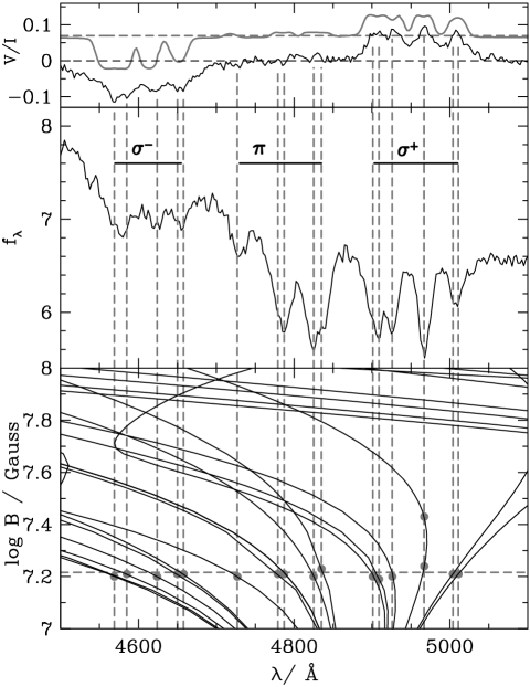
Figure 2: Zeeman maximum ($\phi=0$) flux $f_{\lambda}$ (in units of $10^{-16}$ erg cm^-2 s^-1 $\AA^{-1}$) and circular polarization $V/I$ of HE 1045$-$0908, plotted along with the theoretically predicted field-dependent transition wavelengths ($\lambda$–$B$ curves) for Balmer absorption lines. The top panel also shows a theoretical circular polarization spectrum for a model atmosphere permeated by a homogeneous field of $B=16$ MG (shifted upwards by 0.07 units, with the horizontal dashed grey line denoting the zero polarization level). In the bottom panel, filled circles denote unambiguous identifications of transitions.

2.2 Data analysis

In June 1999, we obtained a sequence of five exposures of HE 1045$-$0908 covering a time interval of 1.7 h, terminated by bad weather. This run yielded two independent circular polarization spectra (Eq. 1). In December 1999, another “snapshot” of two additional exposures was secured, yielding another polarization spectrum. All flux spectra are shown in Fig. 1 (left panel). The temporal change in the five June 1999 spectra is similar to that seen in the data set of Schmidt et al. (2001). In our data, the Zeeman features are most prominent at the beginning of the observations, in the Schmidt et al. data at the end. The features at the beginning and at the end of our run resemble those at the end and the beginning of the Schmidt et al. run, respectively, i. e. the variation of the Zeeman features in our run is reversed with respect to the Schmidt et al. data. Our isolated observation in December 1999 also fits into this pattern. We estimate that the phase of the strongest Zeeman features occurs between our spectra 1 and 2 in Fig. 1. Spectrum 5 approximately corresponds to the phase with the weakest Zeeman features. The implied rotational period is $P_{\mathrm{rot}}$ $\simeq 2.7$ h if the combined Schmidt et al. and present observations cover a full rotational period. While the substantial variation of the Zeeman features suggests this might be true, there is unfortunately no proof of such a connection of the phase intervals covered in the separate observations. Alternatively, it is possible that the Schmidt et al. and our data do not cover a full rotational period and $P_{\mathrm{rot}}$ $>2.7$ h. We refer to the former as case (i) and to the latter as case (ii). In case (ii), there are several possibilities for the phase intervals covered by our and the Schmidt et al. data which we discuss below. The large variation in the strength of the Zeeman features cannot arise in too short a phase interval, however, and we find that for periods in excess of 9 h an acceptable solution is no longer obtained. We follow the suggestion of Schmidt et al. of a period in the 2–4 h range and adopt 2.7 h as the preferred period, but report on the consequences of assuming a longer period below.

In preparation of the analysis, we note that the flux spectra of December 1999 (spectra 6 and 7 in Fig. 1) are very similar in shape to spectrum 5 and provide an additional independent circular polarization spectrum which connects in phase to the June 1999 run. We collect spectra 1/2, 3/4, and 6/7 into three flux and circular polarization rotational phase bins. For case (i) with $P_{\mathrm{rot}}$ $\simeq 2.7$ h, these bins are approximately centred at rotational phases $\phi$ = 0.0, 0.25, and 0.5, where $\phi$ = 0 refers to the phase of maximum strength of the Zeeman features in our June 1999 observation. The case (i) concatenation of our and the Schmidt et al. data requires that the flux spectrum at $\phi$ = 0.75 resembles that at $\phi$ = 0.25. As a representative case (ii), we consider twice the rotational period and tentatively assign the three spectra to $\phi$ = 0.0, 0.125, and 0.25. Our observations now cover a phase interval of only $\Delta\phi$ = 0.25. Furthermore, we adopt $P_{\mathrm{rot}}$ $\simeq 7.5$ h or even 11.3 h and assign the spectra to $\phi$ = 0.0, 0.09, and 0.18 or 0.0, 0.06, and 0.12 with $\Delta\phi$ = 0.18 or 0.12, respectively.

In Fig. 1 (right panel), we present the three flux and circular polarization spectra which form the basis of our tomographic analysis. We refer to the mean of spectra 1 and 2 as “Zeeman maximum” ($\phi=0.0$) and to the mean of spectra 6 and 7 as “Zeeman minimum”, which corresponds to $\phi$ = 0.5 for case (i) and to the smaller values given above for case (ii).

3 Qualitative analysis of the magnetic field geometry

The rich Zeeman spectra of HE 1045$-$0908 allow us to obtain insight into the magnetic field geometry already by the simple means of comparing the spectra with the expected field-dependent wavelengths of the hydrogen transitions $\lambda^{\textrm{H}}(B)$, henceforth referred to as $\lambda$–$B$ curves (Forster et al. 1984; Rösner et al. 1984; Wunner et al. 1985). Fig. 2 shows the wavelength range around H$\beta$ of the Zeeman maximum spectrum ($\phi=0.0$) along with the $\lambda$–$B$ curves. Several transitions that can be immediately identified are marked by filled grey circles. This holds for the $\sigma$ and $\pi$ components in the flux spectrum and the $\sigma$ components in the polarization spectrum, while the circular polarization of the $\pi$ component vanishes, indicating a small viewing angle $\psi$ between the magnetic field direction and the line of sight. The distribution of field strengths is sharply concentrated at $\sim$ 16 MG, as demonstrated also by the fair agreement between the observed and the model polarization spectrum shown at the very top of Fig. 2. This model spectrum is calculated for a single value $B=16$ MG, $\psi=29$°, and $T_{\mathrm{eff}}$ = 10 000 K. Hence, the field over the visible hemisphere at this phase is $\sim$ 16 MG and directed towards us.

The identification of Zeeman transitions is not as easily possible in the Zeeman minimum spectrum ($\phi=0.5$), and we do not show the corresponding attempt of a quick analysis. Four transitions can definitely be identified, however, from almost stationary parts of the $\lambda$–$B$ curves in H$\alpha$ and H$\beta$ $\sigma^{+}$, and the corresponding field strengths span a range from 20 to 60 MG. This simple analysis proves already that the field strength over the stellar surface varies by about a factor four, excluding simple field configurations like a centred or a moderately offset dipole.

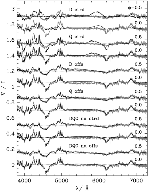
Figure 3: Observed circular polarization spectra for phases $\phi=0.0$ and 0.5 (grey curves) and best-fit synthetic spectra (black curves) for different parametrizations of the magnetic field geometry. From top to bottom: centred dipole (D ctrd); centred quadrupole (Q ctrd); off-centred dipole (D offs); off-centred quadrupole (Q offs); centred, non-aligned combination of dipole, quadrupole, and octupole (DQO na ctrd); off-centred, non-aligned combination of dipole, quadrupole, and octupole (DQO na offs). All curves except for the bottom one have been shifted vertically by suitable amounts in $V/I$, with the horizontal dashed lines indicating the respective levels of zero polarization. The quoted phases refer to case (i) with $P_{\mathrm{rot}}$ = 2.7 h.

Table 2: Best-fit magnetic parameters for the different parametrizations of the magnetic field shown in Fig. 3. The uncertainties in the last digit are denoted by the values in brackets. A short description of the individual models is followed by the formal value of the reduced $\chi^{2}$ (see text). All models assume a rotational period of 2.7 h, except for model (7), which has been computed for 5.4 h.

$i$	$B^{\mathrm{d}}_{\mathrm{pol}}$	$\Theta^{\mathrm{d}}$	$\Phi^{\mathrm{d}}$	$B^{\mathrm{q}}_{\mathrm{pol}}$	$\Theta^{\mathrm{q}}$	$\Phi^{\mathrm{q}}$	$B^{\mathrm{o}}_{\mathrm{pol}}$	$\Theta^{\mathrm{o}}$	$\Phi^{\mathrm{o}}$	${x^{\prime}}_{\mathrm{off}}$	${y^{\prime}}_{\mathrm{off}}$	${z^{\prime}}_{\mathrm{off}}$
(°)	(MG)	(°)	(°)	(MG)	(°)	(°)	(MG)	(°)	(°)	($R_{\mathrm{WD}}$)	($R_{\mathrm{WD}}$)	($R_{\mathrm{WD}}$)
(1) D ctrd (centred dipole, $\chi^{2}_{\mathrm{red}}$ = 121.9)
57 (3)	$-$32 (1)	14 (1)	30 (1)	–	–	–	–	–	–	–	–	–
(2) Q ctrd (centred quadrupole, $\chi^{2}_{\mathrm{red}}$ = 104.9)
11 (2)	–	–	–	$-$36 (1)	14 (1)	18 (1)	–	–	–	–	–	–
(3) D offs (off-centred dipole, $\chi^{2}_{\mathrm{red}}$ = 29.7)
20 (3)	$-$27 (3)	41 (5)	29 (2)	–	–	–	–	–	–	0.08 (1)	0.02 (1)	0.27 (1)
(4) Q offs (off-centred quadrupole, $\chi^{2}_{\mathrm{red}}$ = 27.2)
18 (3)	–	–	–	$-$49 (4)	20 (1)	20 (2)	–	–	–	$-$0.13 (1)	0.01 (1)	0.06 (1)
(5) DQO na ctrd (non-aligned, centred combination of dipole, quadrupole, and octupole, $\chi^{2}_{\mathrm{red}}$ = 26.8)
20 (3)	$-$12 (2)	39 (4)	17 (2)	$-$45 (4)	36 (3)	34 (6)	$-$19 (1)	60 (5)	27 (3)	–	–	–
(6) DQO na offs (non-aligned, off-centred combination of dipole, quadrupole, and octupole, $\chi^{2}_{\mathrm{red}}$ = 24.5)
17 (3)	$-$16 (2)	71 (5)	344 (2)	$-$36 (3)	21 (3)	138 (6)	$-$18 (2)	70 (9)	115 (7)	0.07 (1)	$-$0.08 (1)	0.31 (2)
(7) DQO na offs (non-aligned, off-centred combination of dipole, quadrupole, and octupole, $P_{\mathrm{rot}}$ = 5.4 h, $\chi^{2}_{\mathrm{red}}$ = 26.3)
32 (4)	$-$13 (1)	31 (4)	1 (1)	$-$37 (3)	24 (3)	209 (4)	$-$25 (3)	69 (12)	245 (10)	$-$0.08 (1)	0.07 (1)	0.27 (2)

4 Zeeman tomography of the magnetic field

Theoretical wavelength-dependent Stokes $I$ and $V$ profiles of magnetized white dwarf atmospheres can be computed by solving the radiative transfer equations for given $B$, $\psi$, $T_{\mathrm{eff}}$, $\log g$, and the direction cosine $\mu=\cos\vartheta$, where $\vartheta$ denotes the angle between the normal to the surface and the line of sight. A synthetic spectrum for a given magnetic topology can be described by a superposition of model spectra computed for different parameter values. Our three-dimensional grid of 46 800 $I$ and $V$ model spectra covers 400 $B$ values (1–400 MG, in 1 MG steps), nine $\psi$ values (equidistant in $\cos\psi$), and 13 temperatures (8000–50 000 K) for fixed $\log g$ = 8 and $\mu=1$ (Paper I). This database allows fast computations of synthetic spectra for any given magnetic field configuration without the need to solve the radiative transfer equations each time. Limb darkening is accounted for in an approximate way by the linear interpolation

$$I_{\lambda}(\mu)/I_{\lambda,\mu=1}=a+b\mu\,.$$ (2)

For the sake of simplicity, the temperature- and wavelength-dependencies of $a$ and $b$ have been neglected (see the discussion in Paper I). Fitting the measured absolute flux distribution of HE 1045$-$0908 with model spectra computed using the full radiative transfer method, we find an effective temperature of $T_{\mathrm{eff}}$ = 10 000 $\pm$ 1000 K. For this temperature, model spectra computed as a function of $\mu$ suggest $a=0.53$ and $b=0.47$. In the subsequent tomographic analysis, these values of $T_{\mathrm{eff}}$, $a$, and $b$ were employed and kept constant.

Our Zeeman tomographic code requires an appropriate parametrization of the magnetic field, such that for every location $\@vec{r}$ on the stellar surface the magnetic field vector $\@vec{B}(\@vec{r},\@vec{a})$ can be computed depending on a parameter vector $\@vec{a}=(a_{1},\dots,a_{M})$ of $M$ free parameters describing the field geometry. Best-fit parameters are determined by minimizing a penalty function as a measure for the misfit between model and observation. For that purpose, we employed the C programming language library evoC by Trint & Utecht (1994) which implements an evolutionary minimization strategy. The penalty function we used is the classical reduced $\chi^{2}$

$$\chi^{2}_{\mathrm{red}}(\@vec{a})=\frac{1}{N-M}\sum_{j=1}^{N}\frac{(f_{j}-s_{j}(\@vec{a}))^{2}}{{\sigma_{j}}^{2}}$$ (3)

with the input data pixels $f_{j}$, the model data pixels $s_{j}$, and the standard deviations $\sigma_{j}$. We used 1321 pixels per phase for the individual flux and polarization spectra each, yielding $N=7926$ pixels in total ($\lambda=3900$–7200 Å, $\Delta\lambda=2.5$ Å). All phases have been equally weighted, and flux and circular polarization have also been given equal weight. In order to estimate the statistical noise, a Savitzky-Golay filter with a width of nine pixels (corresponding to 20 Å) has been applied to the observed spectra. Subsequently, the standard deviations $\sigma_{j}$ entering Eq. (3) have been computed from the differences between the filtered and original spectra for wavelength intervals of 250 Å. The standard form of $\chi^{2}_{\mathrm{red}}$ was used as a suitable relative goodness-of-fit measure, but the unavoidable systematic differences between the observed and theoretical spectra prevent that anything near $\chi^{2}_{\mathrm{red}}$ $\simeq 1$ can be achieved.

In order to avoid that such systematic differences influence the analysis of the narrower Zeeman structures, we adjusted the model flux spectra to the observed spectra at a number of wavelengths outside obvious Zeeman features. This procedure improves the fit of the flux spectra to the data but does not affect the polarization spectra. The wavelengths in question are marked by ticks at the top of Fig. 1 (right panel). Due to the finite exposure times, a model spectrum corresponding to a given observed spectrum should in principle be computed from several model spectra covering the respective phase interval. Our code is able to account for this “phase smearing” effect, but the need to compute the additional spectra slows down the minimization procedure so much that we decided against this approach. After having obtained best-fit parameters, we computed spectra including the effect and found no significant differences. The statistical errors of the best-fit parameters have been computed using the method described in Zhang et al. (1986).

Details of the radiative transfer calculations, the synthetisation of model spectra, the geometry adopted for the description of the magnetic field configuration, and the fitting strategy are given in Paper I.

4.1 Field parametrization

In theoretical terms, a magnetic field of very general shape (with the constraints that it is curl-free and generated only in the stellar interior) can be described by expanding the scalar magnetic potential in spherical harmonics depending on the indices $l$ and $m$ for the degree and order of the expansion (Gauß 1838; Langel 1987). For each $(l,m)$-combination, two free parameters $g_{l}^{m}$ and $h_{l}^{m}$ are assigned, while only one parameter, $g_{l}^{0}$, describes the zonal components with $m=0$. Thus, the number of free parameters for an expansion up to degree $l$ is $l(l+2)=15$ (24, 35) for $l=3$ (4, 5), increasing rapidly with the maximum degree $l$. Another property of multipole expansions is the dependence of the degree $l$ required for an adequate description on the choice of the reference axis. Consider, e.g., a non-aligned superposition of a dipole and a quadrupole, which can be described exactly by four parameters ($g_{1}^{0}$, $g_{1}^{1}$, $h_{1}^{1}$, $g_{2}^{0}$) if the reference axis coincides with the axis of symmetry of the quadrupole. If the reference axis points in a different direction, a finite $l$ allows only an approximate description.

In order to ensure stable and fast convergence of our optimization scheme, it is necessary to minimize the number of free parameters. We adopt, therefore, a hybrid model which implements a superposition of zonal ($m=0$) harmonics only, disregarding the other tesseral components with $m\neq 0$. We allow for arbitrary tilt angles of the zonal components and also for off-centre shifts. With this configuration, it is possible to describe fairly complex geometries with fewer parameters than in the truncated multipole expansion which includes all tesseral components (see Paper I for a detailed description).

4.2 Results

4.2.1 Case (i): $P_{\mathrm{rot}}$ = 2.7 h

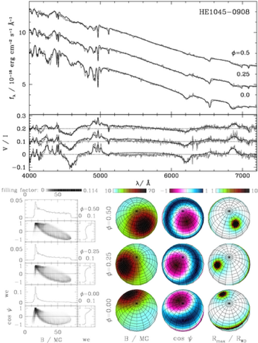
Figure 4: Zeeman tomographic analysis of the magnetic field configuration of HE 1045$-$0908 using a centred, non-aligned combination of dipole, quadrupole, and octupole. Top: Observed (grey curves) and best-fit synthetic spectra (black curves). The uppermost two flux (circular polarization) spectra have been shifted for clarity by 2 and 4 (0.1 and 0.2) units in $f_{\lambda}$ ($V/I$). The quoted phases refer to case (i) with $P_{\mathrm{rot}}$ = 2.7 h. Bottom left: $B$–$\psi$ diagram, bottom right: absolute value of the surface magnetic field, cosine of the angle $\psi$ between the magnetic field direction and the line of sight, and maximum radial distance reached by field lines in units of the white dwarf radius (see text).

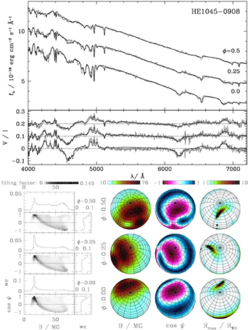
Figure 5: Zeeman tomographic analysis of the magnetic field configuration of HE 1045$-$0908 using an off-centred, non-aligned combination of dipole, quadrupole, and octupole. Top: Observed (grey curves) and best-fit synthetic spectra (black curves). The uppermost two flux (circular polarization) spectra have been shifted for clarity by 2 and 4 (0.1 and 0.2) units in $f_{\lambda}$ ($V/I$). The quoted phases refer to case (i) with $P_{\mathrm{rot}}$ = 2.7 h. Bottom left: $B$–$\psi$ diagram, bottom right: absolute value of the surface magnetic field, cosine of the angle $\psi$ between the magnetic field direction and the line of sight, and maximum radial distance reached by field lines in units of the white dwarf radius (see text).

In an attempt to find the best-fitting field geometry for HE 1045$-$0908, we considered a sequence of parametrizations with increasing complexity. In Fig. 3, we compare the observed circular polarization spectra at $\phi=0.0$ and $\phi=0.5$ with such a sequence of model spectra. The best-fit parameters and the corresponding $\chi^{2}_{\mathrm{red}}$ values are listed in Table 2. For the two simplest configurations (centred dipole and centred quadrupole) we obtained no satisfactory fit to the observations. This can be easily explained by the range of field strengths generated by these configurations, which is too large for $\phi=0.0$ and too small for $\phi=0.5$. It is interesting to note that the centred dipole, which obviously provides the least adequate description, is the only configuration that yields an inclination of $i>20\degr$, whereas for all other configurations an inclination of $i\simeq 10\degr$–20° is obtained.

If an appropriate offset from the stellar centre is introduced for the dipole and quadrupole configurations, the possible range of surface field strengths increases and an extended region with a nearly constant field strength of 16 MG can be generated. Simultaneously, on the opposite stellar hemisphere a smaller high-field region with a steeper field gradient is created. As expected, the off-centred dipole and quadrupole models match the observations better than the centred configurations, with the quadrupole model fitting better than the dipole. In general, however, these simple models are unable to produce adequate fits to all details at all phases simultaneously.

The next steps in complexity of the field configuration are represented by the superposition of dipole, quadrupole, and octupole and the introduction of an off-centre shift. Dipole-quadrupole combinations were not successful and the inclusion of the octupole is essential.

In a first attempt, we allowed the three individual components to be inclined with respect to each other, but not to be offset from the centre. The best fit with this field parametrization matches the observed flux and polarization spectra well for all rotational phases (Fig. 4, top panel). The frequency distribution of field strengths extends from 10 to 70 MG and peaks at 16 MG. At $\phi=0.0$ the distribution of field strengths drops steeply towards lower and higher fields, while at $\phi=0.5$ the peak is less pronounced and the distribution is much broader, implying that fields up to 70 MG contribute significantly to the Zeeman spectra. The $B$–$\psi$ diagram (Fig. 4, bottom left panel) shows that for the fields above 30 MG the sign of $\cos\psi$ is reversed compared with the most frequent field of 16 MG. The picture of the field geometry (Fig. 4, bottom right panel) shows a high-field spot with $B$ up to 70 MG superimposed on a low-field background of 10–20 MG. The field geometry on the visible part of the stellar surface is quadrupole-like with field lines leading from the high-field pole to an “equatorial” band. The field strengths and orientations of the individual components are given in line (5) of Table 2 (see also Eq. 7 in Paper I). With 45 $\pm$ 4 MG, the quadrupole is more than three times as strong as the dipole with 12 $\pm$ 2 MG. The three field components are more or less aligned, with the quadrupole inclined by only 11°, and the octupole by 22° with respect to the dipole. The slight inclinations of the individual components with respect to each other produce the required widening of the high-field spot. Basically, the field structure is that of an oblique rotator with an angle of $\sim$ 40° between field and rotational axes. The lower right panel, labelled $R_{\mathrm{max}}/R_{\mathrm{WD}}$, indicates the maximum radial distances to which field lines extend in units of the white dwarf radius. Distances beyond 10 $R_{\mathrm{WD}}$ (black) may denote open field lines.

A slightly better fit is obtained if we allow for a common offset from the centre for all three components. As can be seen from Fig. 5 (top panel), this additional freedom leads, in particular, to improvements in the model circular polarization which we consider significant: (i) the steep rise at 4170–4220 Å for $\phi=0.0$; (ii) the dips at 4790–4870 Å and at 5300 Å for $\phi=0.5$; and (iii) the continuum polarization in the 5200–6000 Å range. The $B$–$\psi$ diagram (Fig. 5, bottom left panel) shows an enhanced frequency of field strengths around 60 MG for all three phases. For $\phi=0.5$ we still see a pronounced decrease at 70 MG, but, in contrast to the previous configuration, there is a small but significant contribution from fields of 70–76 MG and the same direction as the prevailing field of 16 MG. Figure 5 (bottom right panel) shows a field geometry that is similar from a global point of view, but reveals a more complex structure in the high-field region with two separate areas of opposite field direction. This general similarity is produced, however, by an arrangement of the field components which is entirely different from the previous model (see also the examples given in Paper I). The quadrupole is now inclined by 90° with respect to the dipole, and the octupole is not far from orthogonal to both. The shift is primarily in the direction of the dipole ($z^{\prime}$-axis), and, hence, shifts the quadrupole perpendicularly to its axis. The field strengths quoted for this model in line (6) of Table 2 refer to the unshifted components, and the final surface values can be calculated with some additional algebra. The shape of the region with field lines reaching beyond 10 $R_{\mathrm{WD}}$ (black) has changed from a circular spot to an arc. Field lines still end in a linearly extended region just visible at the stellar limb for $\phi=0.0$.

All models in lines (1) through (6) of Table 2 have the property that the $\phi=0.75$ Zeeman spectra resemble those at $\phi=0.25$, as required by the proposed concatenation of the Schmidt et al. and our data. Hence, although the Schmidt et al. data have not been used in the fit, they are approximately reproduced by the models.

The models of lines (5) and (6) of Table 2 with 9 and 12 free field parameters, respectively, fit better than the 17-parameter model of the full multipole expansion up to $l=3$ presented in a preliminary report (Euchner et al. 2005). While this multipole expansion provides a better fit, e. g., to the 5200–6000 Å continuum polarization at $\phi=0.0$, it fails more seriously in other places. It seems that the choice of the arbitrarily oriented zonal components is more adequate for the case of HE 1045$-$0908. Models with about a dozen free magnetic field parameters represent the present limit of our code at which a stable convergence to the global minimum in the $\chi^{2}$ landscape can be achieved.

The general agreement between the observed and synthetic flux and polarization spectra has reached a high level which indicates that the theoretical spectra describe the underlying physics of magnetic atmospheres more or less correctly by now. The remaining differences can be traced back to a number of sources. On the theoretical side these are: (i) uncertainties in the absorption coefficients and approximations in the treatment of the line broadening, in particular, the treatment of Stark broadening in magnetic atmospheres; (ii) the finite resolution of the database, currently limited to 1 MG, which causes small wiggles in the spectra. On the observational side these are: (iii) remaining problems with the flux calibration, i.e. in the observationally derived response functions, which we have attempted to correct for by re-normalizing the observed and model spectra relative to each other; (iv) small errors in the flat fielding procedure; and (v) uncertainties in the definition of the standard deviations $\sigma_{j}$ of spectral flux and polarization which enter Eq. (3) and determine $\chi^{2}_{\mathrm{red}}$.

4.2.2 Case (ii): $P_{\mathrm{rot}}$ $>2.7$ h

We have repeated the analysis for rotational periods exceeding the preferred value of 2.7 h, in order to investigate whether the assumption of a longer period, which implies incomplete phase coverage, leads to a different field structure. The somewhat surprising, but also fortunate result is that none of the investigated models yields a field structure which deviates substantially from the one derived above.

We replace the assumed value 0.50 of the phase interval $\Delta\phi$ covered by our data by 0.25, 0.18, and 0.12, corresponding to rotational periods of 5.4 h, 7.5 h, and 11.3 h. We consider first the case of $P_{\mathrm{rot}}$ = 5.4 h. The important finding is that the assumption $\Delta\phi$ = 0.25 does not imply the occurrence of a double wave of full period 5.4 h in the Zeeman features, but rather a field structure similar to case (i) seen at the larger inclination of $i\simeq 32$°. At least, this is true for our models which lack multipole components higher than the octupole. As an example, we list in Table 2, line (7), the parameters for a non-aligned, off-centred dipole-quadrupole-octupole combination with an assumed period of 5.4 h, which should be compared with the model in line (6) for our preferred period of 2.7 h. For both models, the Schmidt et al. and our data are concatenated at the phase of Zeeman maximum, but in line (6) the combined data cover a full rotational period, and in line (7) only half a period. We conclude that the dominance of the quadrupole and octupole over the dipole is not affected by the different choice of the rotational period.

The case (ii) model with $\Delta\phi$ = 0.18 requires an inclination of $i$ = 34°, whereas for $\Delta\phi$ = 0.12 (with $i$ = 53°) a satisfactory fit could no longer be obtained. This suggests a maximum value of the rotational period of about 9 h. It is not surprising that for decreasing $\Delta\phi$ the necessary field variation between Zeeman maximum and minimum can only be produced by larger inclinations which allow for a more rapid variation of the Zeeman features.

5 Discussion

In this study, we have fitted model Zeeman spectra to high-quality spectropolarimetric data of HE 1045$-$0908 using our Zeeman tomography code (Paper I), assuming a bona fide rotational period of about 2.7 h. We have achieved a good fit which reveals a dominant quadrupole component with additional dipole and octupole contributions. HE 1045$-$0908 is the first white dwarf in which a quadrupole component has been detected so clearly. This result is found to be robust against the assumption of a longer rotational period with an upper limit at about 9 h. In our model, the orientations of the axes of dipole, quadrupole, and octupole have been treated as free parameters, and it turned out that this freedom is important in obtaining the best fit. This assumption deviates from a truncated multipole expansion with all $m\neq 0$ components and is justified by its simplicity and ease of visualization. We are confident that we have reached a reliable reconstruction of the general field structure of HE 1045$-$0908.

The most frequent photospheric field strength and direction is represented by the maximum in the $B$–$\psi$ diagram at 16 MG and positive cos $\psi$. This is also the field which appears most prominently in the Zeeman spectra, and a cursory analysis would catalogue this star as “having a field strength of 16 MG”. Other sections of the star display field strengths up to $\sim$ 75 MG, however, which are less conspicuous in the observed spectra. Considering the complete information on the field distribution, we find it difficult to assign either a “characteristic field strength” or a “polar field strength” to HE 1045$-$0908. More appropriate would be quotations like: (i) the most frequent field is 16 MG; (ii) the mean field over the visible surface averaged by the surface area is 34 MG; and (iii) the range of field strengths is 10–75 MG. Our general experience is, however, that a quotation of type (iii) is model-dependent because models for some stars studied by us imply a high-field extension in the $B$–$\psi$ diagram, which covers only a small area near the limb of the visible surface and has little statistical significance.

The derived field structure of HE 1045$-$0908 is primarily defined by the $B$–$\psi$ diagram rather than by the strengths and angles of the individual components. As pointed out in Paper I, different parameter combinations of the individual components could lead to a similar $B$–$\psi$ diagram. This is why Donati et al. (1994) refrained from specifying multipole components and suggested to directly optimize the $B$–$\psi$ diagram. The approach of Donati et al. does not guarantee, however, that the derived $B$–$\psi$ diagram corresponds to a physically possible field. This potential trap is avoided in our approach, which has the additional advantage that we can specify the contributions of individual multipole components. Furthermore, since we have gradually increased the level of complexity of our field parametrization starting from the elementary case of a centred dipole, we can be sure to have found the simplest configuration compatible with the observations. We cannot exclude additional small scale structure of the surface field, but suggest that such a structure cannot dominante HE 1045$-$0908 because it would destroy the remarkably high degree of circular polarization of up to $\sim$ 10 %.

Due to the small inclination ($i$ = 17°) found for the best-fitting model geometry, a fraction of 35 % of the stellar surface is permanently hidden from view. In Paper I we have shown that this lack of information does not affect the accuracy of the derived field structure on the visible part of the surface. The field structures predicted by all our models for the hidden part of the surface are reasonable and “well-behaved”, i. e. there are no extreme field values or gradients. For instance, for the case (i) model of Fig. 5 and line (6) of Table 2, the range of field strenghts encountered on the visible fraction of the surface is 10–76 MG, while for the whole star it is 9–76 MG. Our simulations had shown that reconstruction artefacts can arise if the field parametrization involves more free parameters than needed to describe the field structure adequately (cf. Fig. 10 in Paper I). This does not happen in our stepwise approach with a limited number of parameters.

It goes without saying that the final determination of the field structure of HE 1045$-$0908 would greatly benefit from a measurement of its rotational period and full phase coverage of the Zeeman spectropolarimetry.

With $T_{\mathrm{eff}}$ $\simeq 10^{4}$ K, HE 1045$-$0908 is $\sim$ 0.5 Gyr old, less than the Ohmic decay times of the detected multipole components (Wendell et al. 1987; Cumming 2002). Hence, the strong quadrupole component could be a remnant from the main-sequence (or pre-main-sequence) evolution of the progenitor star. Alternatively, it could be produced by field evolution in the white dwarf stage as suggested by Muslimov et al. (1995). Now that tomographic methods have reached a high accuracy thanks to advanced spectropolarimetric instruments at 8-m class telescopes, it would be interesting to follow up this question by a detailed field analysis of white dwarfs of different ages, supplemented by more extensive theoretical calculations of the evolution of white dwarf magnetic fields over their cooling times.