DENSITY POWER SPECTRUM OF COMPRESSIBLE HYDRODYNAMIC TURBULENT FLOWS

Abstract

Turbulent flows are ubiquitous in astrophysical environments, and understanding density structures and their statistics in turbulent media is of great importance in astrophysics. In this paper, we study the density power spectra, $P_{\rho}$, of transonic and supersonic turbulent flows through one and three-dimensional simulations of driven, isothermal hydrodynamic turbulence with root-mean-square Mach number in the range of $1\lesssim M_{\rm rms}\lesssim 10$. From one-dimensional experiments we find that the slope of the density power spectra becomes gradually shallower as the rms Mach number increases. It is because the density distribution transforms from the profile with discontinuities having $P_{\rho}\propto k^{-2}$ for $M_{\rm rms}\sim 1$ to the profile with peaks having $P_{\rho}\propto k^{0}$ for $M_{\rm rms}\gg 1$. We also find that the same trend is carried to three-dimension; that is, the density power spectrum flattens as the Mach number increases. But the density power spectrum of the flow with $M_{\rm rms}\sim 1$ has the Kolmogorov slope. The flattening is the consequence of the dominant density structures of filaments and sheets. Observations have claimed different slopes of density power spectra for electron density and cold H I gas in the interstellar medium. We argue that while the Kolmogorov spectrum for electron density reflects the transonic turbulence of $M_{\rm rms}\sim 1$ in the warm ionized medium, the shallower spectrum of cold H I gas reflects the supersonic turbulence of $M_{\rm rms}\sim$ a few in the cold neutral medium.

1 INTRODUCTION

According to the currently accepted paradigm, the interstellar medium (ISM) is in a state of turbulence and the turbulence is believed to play an important role in shaping complex structures of velocity and density distributions (see, e.g., Vázquez-Semadeni et al., 2000; Elmegreen & Scalo, 2004, for reviews). The ISM turbulence is transonic or supersonic with Mach number varying from place to place; while the turbulent Mach number, $M$, is probably of order unity in the warm ionized medium (WIM) judging from the temperature that ranges from $6\times 10^{3}$ to $10^{4}$ K (Haffner et al., 1999), it is a few in the cold neutral medium (CNM) (e.g., Heiles & Troland, 2003) and as large as 10 or higher in molecular clouds (e.g., Larson, 1981). The fact that $M\gtrsim 1$ implies high compressibility, and observations of the ISM reflect the density structures resulted from the turbulence. Interpreting these observations and hence understanding the density structures require a good knowledge of density statistics.

Density power spectrum, $P_{\rho}$, is a statistics that can be directly extracted from observations. The best-known density power spectrum of the ISM is the one presented in Armstrong et al. (1981, 1995). It is a composite power spectrum of electron density collected from observations of velocity fluctuations of the interstellar gas, rotation measures, dispersion measures, interstellar scintillations and others. What is remarkable is that a single Kolmogorov slope of $-5/3$ fits the power spectrum for the wavenumbers spanning more than 10 decades. But there are also a number of observations that indicate shallower spectra. For instance, Deshpande et al. (2000) showed that the density power spectrum of cold H I gas has a much shallower slope of $-0.75\sim-0.5$. Here we note that the power spectrum of Armstrong et al. (1981, 1995) should reveal density fluctuations preferably in the WIM since it is for the electron density. On the other hand, the power spectrum of Deshpande et al. (2000) represents the so-called tiny-scale atomic structure in the CNM (Heiles, 1997).

Discussions on density power spectrum in the context of theoretical works have been scarce. It is partly because the study of turbulence was initiated in the incompressible limit. Instead velocity power spectrum was discussed extensively by comparing the well-known theoretical spectra, such as those of Kolmogorov (1941) and Goldreich & Sridhar (1995). Hence, although hydrodynamic or magnetohydrodynamic (MHD) simulations of compressible turbulence were performed, the spectral analysis was focused mainly on velocity (and magnetic field in MHDs) (e.g., Cho & Lazarian, 2002; Vestuto et al., 2003). A few recent simulation studies, however, have reported density power spectrum (e.g., Padoan et al., 2004; Kritsuk et al., 2004; Beresnyak et al., 2005). For instance, in an effort to constrain the average magnetic field strength in molecular cloud complexes, Padoan et al. (2004) have simulated MHD turbulence of root-mean-square sonic Mach number $M_{\rm rms}=10$ with weak and equipartition magnetic fields. They have found that the slope of density power spectrum is steeper in the weak, super-Alfvénic case than in the equipartition case, and super-Alfvénic turbulence may be more consistent with observations. Although their work has focused on the dependence of the slope of density power spectrum on Alfvénic Mach number, they have also demonstrated that the slope is much shallower than the Kolmogorov slope. Kritsuk et al. (2004) and Beresnyak et al. (2005) have found consistently shallow slopes. However, none of the above studies have yet systematically investigated the dependency of the slope of density power spectrum on sonic Mach number.

A note worthwhile to make is that the functional form of probability distribution function (PDF) on the density field of compressible turbulent flows is well established. Passot & Vázquez-Semadeni (1998), by performing one-dimensional isothermal hydrodynamic simulations, have shown that the density PDF follows a log-normal distribution. A few groups (e.g., Nordlund & Padoan, 1999; Ostriker et al., 2001) have reported that the log-normal distribution still holds in three-dimensional isothermal turbulent flows even though the scaling of the standard deviation with respect to rms Mach number is not necessarily the same as the one obtained by Passot & Vázquez-Semadeni (1998).

In this paper we study the density distribution and the density power spectrum in transonic and supersonic turbulent flows using one and three-dimensional hydrodynamic simulations. Specifically we show that the Mach number is an important parameter that characterizes the density power spectrum. The plan of the paper is as follows. In §2 a brief description on numerical details is given. Results are presented in §3, followed by summary and discussion in §4.

2 SIMULATIONS

Isothermal, compressible hydrodynamic turbulence was simulated using a code based on the total variation diminishing scheme (Kim et al., 1999). Starting from an initially uniform medium with density $\rho_{o}$ and isothermal sound speed $a$ in a box of size $L$, the turbulence was driven, following the usual procedure (e.g., Mac Low, 1999); velocity perturbations were added at every $\Delta t=0.001L/a$, which were drawn from a Gaussian random field determined by the top-hat power distribution in a narrow wavenumber range of $1\leq k\leq 2$. The dimensionless wavenumber is defined as $k\equiv L/\lambda$, which counts the number of waves with wavelength $\lambda$ inside $L$. The amplitude of perturbations was fixed in such a way that $M_{\rm rms}$ of the resulting flows ranges approximately from 1 to 10. Self-gravity was ignored.

One and three-dimensional numerical simulations were performed with 8196 and $512^{3}$ grid zones, respectively. We note that one-dimensional turbulence has compressible mode only but no rotational mode, and so its application to real situations is limited. However, there are two advantages: 1) high-resolution can be achieved, resulting in a wide inertial range of power spectra and 2) the structures formed can be easily visualized and understood. In the three-dimensional experiments the driving of turbulence was enforced to be incompressible by removing the compressible part in the Fourier space, although our results are not sensitive to the details of driving. Table 1 summarizes the model parameters.

3 RESULTS

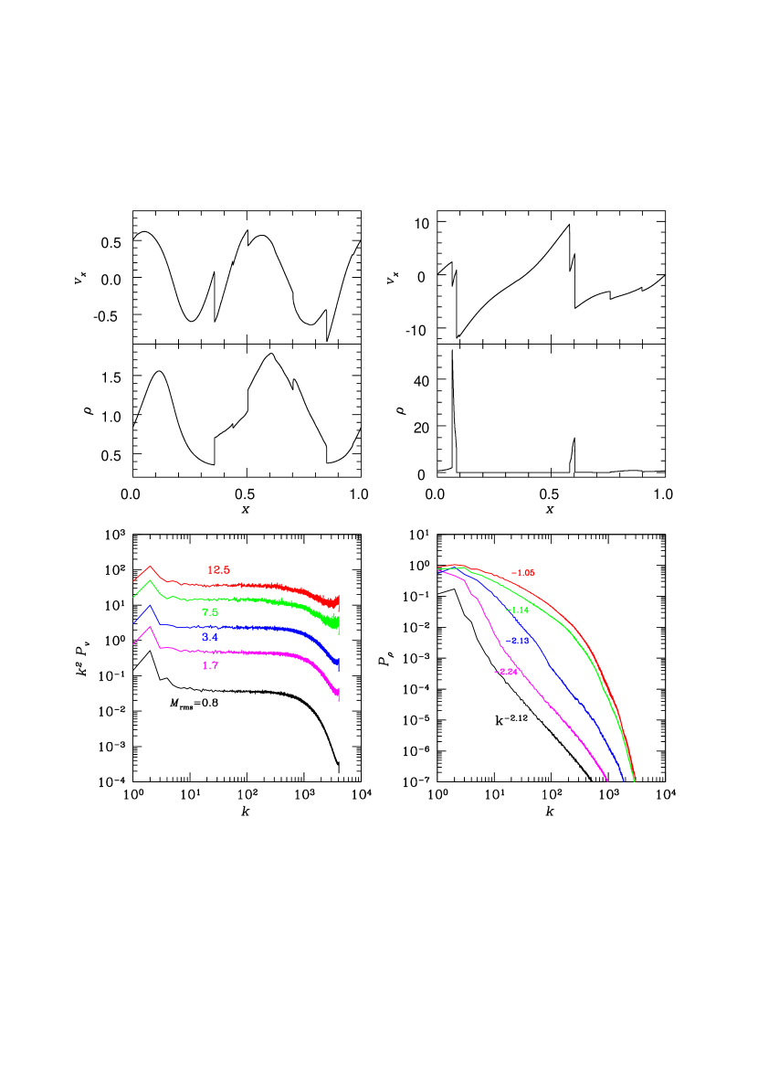
Figure 1: One-dimensional turbulence. Top panels: Snapshots of the spatial profiles of velocity and density, after turbulence was fully saturated, for a transonic turbulence with time averaged $M_{\rm rms}=0.8$ (left) and a supersonic turbulence with time averaged $M_{\rm rms}=12.5$ (right). The plotted quantities are normalized by the isothermal sound speed and the initial density, respectively. Bottom panels: Time-averaged power spectra of velocity (left) and density (right) for flows with different $M_{\rm rms}$’s. The velocity power spectrum in the left panel is multiplied by $k^{2}$ for clarity. Slopes in the right panel were obtained by least-square fits over the range of $20\leq k\leq 60$. Simulations used 8196 grids zones.

Figure 1 presents the results of one-dimensional simulations. Top two panels are snapshots of the spatial profiles of velocity and density for a transonic turbulence with $M_{\rm rms}=0.8$ (left) and a supersonic turbulence $M_{\rm rms}=12.5$ (right). Shocks are developed in both cases, but weak shocks in the transonic case and strong shocks in the supersonic case. The velocity profile shows shock discontinuities, superimposed on the background that reminisces the $k=1$ and $2$ driving. Especially, the supersonic case exhibits the so-called sawtooth profile, which is expected in the turbulence dominated by shocks. Like the velocity profile, the density profile for the transonic case shows shock discontinuities. But the density profile for the supersonic case shows high peaks, which can be understood as follows. Since the density jump is proportional to the square of Mach number in isothermal shocks, the density contrast at high Mach number shocks is very large. With the total mass conserved, the fluid should be concentrated at shock discontinuities producing a peak-dominated profile.

Bottom two panels of Figure 1 show the time-averaged power spectra of velocity (left) and density (right) for flows with different $M_{\rm rms}$’s (see Table 1 for the time interval for averaging). We note that the statistical errors (or standard deviations) of the spectra, which are not drawn in the figure, easily exceed the averaged values, themselves. This is partially due to the fact that the statistical sample is small in one-dimensional experiments. The slope of the velocity power spectra is nearly equal to $-2$, irrespective of rms Mach numbers, as shown in the bottom-left panel. On the contrary, while the slope of the density power spectrum is close to $\sim-2$ for transonic and mildly supersonic flows, it is much shallower for supersonic flows with $M_{\rm rms}=7.5$ and 12.5. Such power spectrum reflects the profiles in the top panels. We note that discontinuities (i.e., step functions) and infinitely thin peaks (i.e., delta-functions) in spatial distribution result in $P_{\rho}\propto k^{-2}$ and $P_{\rho}\propto k^{0}$, respectively. Hence while the density profiles with discontinuities for transonic flows give power spectra with slopes close to $-2$, the profiles with peaks for highly supersonic flows give shallower spectra.

Interestingly $P_{\rho}\propto k^{-2}$ and $P_{\rho}\propto k^{0}$ were predicted in the context of the Burgers turbulence. It is known that the Burgers equation describes a one-dimensional turbulence with randomly developed shocks, and the resulting sawtooth profile gives to the $k^{-2}$ velocity power spectrum, i.e., $P_{v}\propto k^{-2}$ (see, e.g., Fournier & Frisch, 1983). Expanding it, Saichev & Woyczynski (1996) developed a model for the description of density advected in a velocity field governed by the Burgers equation. They showed that in the limit of negligible pressure force (i.e., for strong shocks), all the mass concentrates at shock discontinuities and the density power spectrum becomes $P_{\rho}\propto k^{0}$. In the presence of pressure force (i.e., for weak shocks) their density power spectrum is $P_{\rho}\propto k^{-2}$. Our results agree with those of Saichev & Woyczynski (1996), although ours are based on numerical simulations using full hydrodynamic equations (under the assumption of isothermal flows).

The flattening of density power spectrum for supersonic turbulence is also seen in three-dimensional experiments. The results are presented in Figure 2. Top and middle panels show the density distribution in a two-dimensional slice for a transonic turbulence with $M_{\rm rms}=1.2$ (top) and a supersonic turbulence with $M_{\rm rms}=12$ (middle). The images reveal different morphologies for the two cases. The transonic image includes curves of discontinuities, which are surfaces of shocks with density jump of a few. So the three-dimensional density distribution should contain surfaces of discontinuities on the top of smooth turbulent background. On the other hand, the supersonic image shows mostly density concentrations of string and dot shapes, which are sheets and filaments in three-dimension. Hence, the three-dimensional density distribution should be dominated by sheets and filaments of high density concentration.

Bottom panel of Figure 2 shows the time-averaged density power spectra for flows with different $M_{\rm rms}$’s, along with fitted values of slope (see Table 1 for the time interval for averaging). As in one-dimensional experiments, the slope over the inertial range becomes shallow as the Mach number increases. But unlike in one-dimension, the slope for the transonic turbulence with $M_{\rm rms}=1.2$ is $-1.73$, close to the Kolmogorov value of $-5/3$. It is because the power spectrum represents the fluctuations of turbulent background, rather than discontinuities of weak shocks. Note that in three-dimension turbulence has the rotational mode of eddy motions in addition to the compressional mode of sound waves and shock discontinuities, and the normal cascade is allowed. In supersonic turbulence, we get the slopes of $-1.08$, $-0.75$ and $-0.52$ for $M_{\rm rms}=3.4$, $7.3$ and $12.0$, respectively. Again the shallow spectrum reflects the highly concentrated density distribution, but for this time, of sheet and filament morphology shown in the middle panel. Like delta-functions, infinitely thin sheets and filaments in three-dimension give $P_{\rho}\propto k^{0}$.

As pointed in Introduction, a few recent studies of turbulence have published the slope of density power spectrum: for instance, Padoan et al. (2004) have found a slope of $-0.71$ for $M_{\rm rms}=10$ MHD turbulence with weak magnetic field, and Kritsuk et al. (2004) have found a slope of $-0.88$ for $M_{\rm rms}=6$ hydrodynamic turbulence. We notes that these values are well consistent with ours.

4 SUMMARY AND DISCUSSION

We present the density distribution and the density power spectrum of driven, isothermal, compressible hydrodynamic turbulence in one and three-dimensional numerical experiments. The rms Mach number of flows covers from $\sim 1$ (transonic) to $\sim 10$ (highly supersonic). Our main findings are summarized as follows.
1. In transonic turbulence, the density distribution is characterized by discontinuities generated by weak shocks on the top of turbulent background. On the other hand, in supersonic turbulence with $M_{\rm rms}\gg 1$, it is characterized by peaks or concentrations of mass generated by strong shocks. Those density concentrations appear as sheets and filaments in three-dimension.
2. In three-dimension, the slope of density power spectrum for transonic turbulence with $M_{\rm rms}=1.2$ is $-1.73$, which is close to the Kolmogorov slope of $-5/3$. But as the rms Mach number increases, the slope flattens, reflecting the development of sheet-like and filamentary density structures. The slopes of supersonic turbulence with $M_{\rm rms}=3.4$, $7.3$ and $12.0$ are $-1.08$, $-0.75$ and $-0.52$, respectively.

In Introduction, we have pointed that in the ISM the power spectrum of electron density has the Kolmogorov slope (Armstrong et al., 1981, 1995), whereas the power spectrum of H I gas shows a shallower slope (Deshpande et al., 2000). Our results suggest the reconciliation of these claims of different spectral slopes. That is, the electron density power spectrum represents the density fluctuations mostly in the WIM, where the turbulence is transonic and the density power spectrum has the Kolmogorov slope. On the other hand, the H I power spectrum represents the tiny-scale atomic structures in the CNM, where the turbulence is supersonic with $M_{\rm rms}\sim$ a few and the density power spectrum has a shallower slope.

Through 21cm H I observations, it has been pointed that sheets and filaments could be the dominated density structure in the CNM (e.g., Heiles, 1997; Heiles & Troland, 2003). Our study demonstrates that sheets and filaments are indeed the natural morphological structures in the media with supersonic turbulence such as the CNM.

In this work we demonstrate that the slope of density power spectrum becomes shallow as the rms Mach number increases by considering the simplest possible physics, i.e., by neglecting magnetic field and self-gravity and assuming isothermality. We point, however, that those physics could affect the quantitative results. For instance, the magnetic field, which is dynamically important in the ISM, could further shallow the density power spectrum, as Padoan et al. (2004) have shown. In addition, self-gravity could affect the power spectrum significantly, since it forms clumps and causes the density power spectrum to become flatter or even to have positive slopes. Finally, cooling could make a difference too, especially in the turbulence in the WIM, and may even enhance compressibility, although, as a first order approximation, the assumption of isothermality would be adequate in molecular clouds (see, e.g., Pavlovski et al., 2005).

Table 1: Model Parameters

Model	$\stackrel{{\scriptstyle\cdot}}{{E}}_{\rm kin}$	$t_{\rm end}$	$dt_{\rm output}$	$\Delta t_{\rm sp}$	Resolution
1D0.8	0.1	8	0.1	4-8	8196
1D1.7	1	8	0.1	4-8	8196
1D3.4	10	8	0.1	4-8	8196
1D7.5	100	8	0.1	4-8	8196
1D12.5	400	8	0.1	4-8	8196
3D1.2	1	4.8	0.4	1.2-4.8	$512^{3}$
3D3.4	30	1.5	0.1	0.6-1.5	$512^{3}$
3D7.3	300	1.0	0.05	0.5-1.0	$512^{3}$
3D12.0	1300	0.5	0.05	0.3-0.5	$512^{3}$

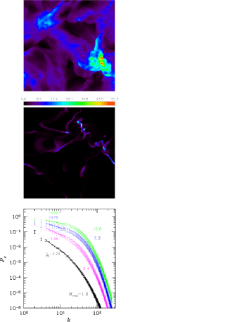
Figure 2: Three-dimensional turbulence. Top and middle panels: Color images of the density distribution in a two-dimensional slice, after turbulence was fully saturated, for a transonic turbulence with time averaged $M_{\rm rms}=1.2$ (top) and a supersonic turbulence with time averaged $M_{\rm rms}=12$ (middle). The color is coded on linear scales and the range of density is an order of magnitude larger for the supersonic case than for the transonic case. Bottom panel: Statistical error bars of the time-averaged density power spectra for flows with different $M_{\rm rms}$’s. Solid lines and their slopes, which were obtained by least-square fits over the range of $4\leq k\leq 14$, are included. Simulations used $512^{3}$ grids zones.

References

- Armstrong et al. (1981) Armstrong, J. W., Cordes, J. M. & Rickett, B. J. 1981, Nature, 291, 561
- Armstrong et al. (1995) Armstrong, J. W., Rickett, B. J. & Spangler, S. R. 1995, ApJ, 443, 209
- Beresnyak et al. (2005) Beresnyak, A., Lazarian, A. & Cho, J. 2005, ApJ, 624, L93
- Cho & Lazarian (2002) Cho, J. & Lazarian, A. 2002, Phys. Rev. Lett., 88, 245001
- Deshpande et al. (2000) Deshpande, A. A., Dwarakanath, K. S. & Goss, W. M. 2000, ApJ, 543, 227
- Elmegreen & Scalo (2004) Elmegreen, B. G. & Scalo, J. 2004, ARA&A, 42, 211
- Fournier & Frisch (1983) Fournier, J. D. & Frisch, U. 1983, J. Mec. Theor. Appl., 2, 699
- Goldreich & Sridhar (1995) Goldreich, P. & Sridhar, H. ApJ, 438, 763
- Haffner et al. (1999) Haffner, L. M., Reynolds, R. J. & Tufte, S. L. 1999, ApJ, 523, 223
- Heiles (1997) Heiles, C. 1997, ApJ, 481, 193
- Heiles & Troland (2003) Heiles, C. & Troland, T. H. 2003, ApJ, 586, 1067
- Kim et al. (1999) Kim, J., Ryu, D., Jones, T. W. & Hong, S. S. 1999, ApJ, 514, 506
- Kolmogorov (1941) Kolmogorov, A. 1941, Dokl. Akad. Nauk SSSR, 31, 538
- Kritsuk et al. (2004) Kritsuk, A., Norman, M. & Padoan, P. 2004 (astro-ph0411626)
- Larson (1981) Larson, R. B. 1981, MNRAS, 194, 809
- Mac Low (1999) Mac Low, M.-M. 1999, ApJ, 524, 169
- Nordlund & Padoan (1999) Nordlund, Å. & Padoan, P. 1999, in Interstellar Turbulence, eds. J. Franco & A. Carramiñana (Cambridge: Cambridge Univ. Press), 218
- Ostriker et al. (2001) Ostriker, E. C., Stone, J. M. & Gammie, C. F. 2001, ApJ, 546, 980
- Pavlovski et al. (2005) Pavlovski, G., Smith, M. D. & Mac Low, M.-M. 2005 (astro-ph/0504504)
- Padoan et al. (2004) Padoan, P., Jimenez, R., Juvela, M. & Nordlund, Å. 2004, ApJ, 604, L49
- Passot & Vázquez-Semadeni (1998) Passot, T. & Vázquez-Semadeni, E. 1998, Phys. Rev. E, 58, 4501
- Saichev & Woyczynski (1996) Saichev, A. I. & Woyczynski, W. A. 1996, SIAM J. Appl. Math., 56, 1008
- Vázquez-Semadeni et al. (2000) Vázquez-Semadeni, E., Ostriker, E. C., Passot, T., Gammie, C. F. & Stone, J. M. 2000, in Protostars and Planets IV, eds. V, Mannings, A. P. Boss & S. S. Russell (Tuscon: University of Arizona Press), p 3
- Vestuto et al. (2003) Vestuto, J. G., Ostriker, E. C. & Stone, J. M. 2003, ApJ, 590, 858