Presenter: P. Bauleo (bauleo@lamar.colostate.edu), usa-bauleo-PM-abs2-he14-poster

Measurement of the Lateral Distribution Function of UHECR Air Showers with the Pierre Auger Observatory

1 Introduction

The Pierre Auger Observatory [1] is being used to study cosmic rays with energies larger than $10^{19}\,\mathrm{eV}$ with unprecedented precision and statistics. An essential quantity that must be deduced from data is the lateral distribution function (LDF) that describes the decreasing of the signals in the water-tanks as a function of distance. Knowledge of the LDF is important for the reconstruction of the shower core and the shower direction. It can also be compared with model calculations to give useful information relating to primary mass. Here we describe how the LDF is measured using the large sample of events recorded with the surface detector (SD) array and with a small sample observed with the fluorescence detectors (FD). For hybrid events, in which SD and FD measurements of the same shower are available, the core position is much better constrained than for SD-only events, thus providing an important cross-check on the LDF determined from SD measurements alone.

2 The Fitting Method

The water-Cherenkov detectors provide information about Cherenkov photons, which are produced when charged particles cross the tanks. The number of Cherenkov photons collected is to a good approximation proportional to the energy deposit in the tank. The signal is calibrated in units of vertical equivalent muons (VEM) [9]. The energy deposit, however, depends strongly on the particle type and the conversion from the Cherenkov signal back to the number of particles in the tank is not obvious. For large tank signals ($>15\,\mathrm{VEM}$) this is not crucial since the uncertainty $\sigma(S)$ of a signal $S$ (in VEM) was determined from data of two detectors positioned 11 meters apart [5] to be $\sigma(S)=1.06\ \sqrt{S}$. But for small tank signals the number of effective particles, $n$, is needed since their Poissonian fluctuation dominates the uncertainty of the signal and is required for the maximum likelihood fit. We have introduced a function that gives $n$ for a measured signal $S(r)$: $n=P(r,\theta,E,A)\times S(r)$ where the conversion factor P is called the Poisson factor and is presently assumed to be independent of the primary energy, $E$, and mass, $A$, for any distance, $r$, and zenith angle, $\theta$. The factor reflects the different energy deposits of different secondaries and is determined by simulations. Finally we set up a maximum likelihood fit to determine the parameters of a trial LDF functional form and, at the same time, the position of the shower core, by comparing each tank signal, with its fluctuations, to the value expected from the trial function, $S_{th}$. $L=\prod_{i}f_{\text{P}}(n_{i},\mu_{i})\times\prod_{k}f_{\text{G}}(n_{k},\mu_{k})\times\prod_{l}F_{\text{sat}}(n_{l},\mu_{l})\times\prod_{m}F_{\text{zero}}(n_{m},\mu_{m}).$ The individual factors of the likelihood function are determined using the information of tanks at their respective distance $r$. The Poissonian probability density, $f_{\text{P}}(n_{i},\mu_{i})$, is calculated for small signals ($S_{i}<15\,\mathrm{VEM}$). For larger signals the Gaussian approximation is used, $f_{\text{G}}(n_{k},\mu_{k})$. The effective particle number $n$ of a saturated tank represents a lower limit of the actual signal and we have to integrate $f_{\text{G}}$ over all possible values larger than $n$, to estimate the detecting probability of a signal larger than $n$. In case of tanks without a signal we have to sum over all Poissonian probabilities with a predicted particle number $\mu_{i}$ and actual effective particle number $n_{i}\leq 3$.

3 LDF Measurements

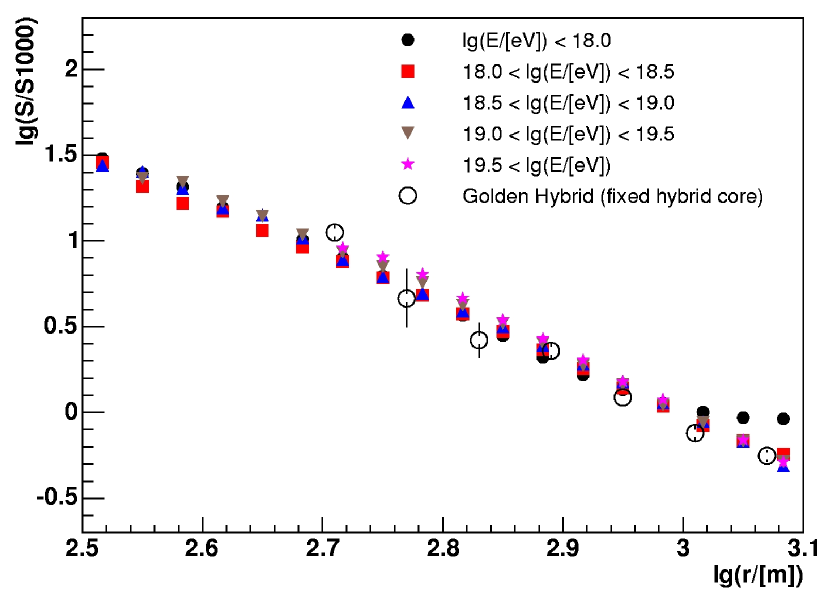
Figure 1: Averaged LDF for $\sec\theta\in[1.2,1.4]$ (NKG fit and floating slope).

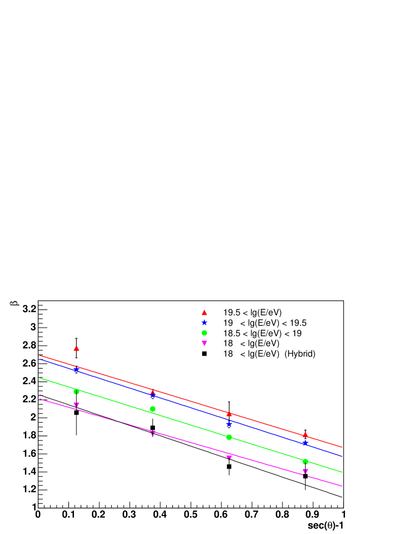
Figure 2: Slope $\beta$ vs zenith angle as function of energy for SD-only or hybrid geometry. Fits to the slope parameter for different energy bins are shown

In contrast to S(1000) the shape of the lateral distribution does not change much with energy [8]. Therefore, the normalisation constant is decoupled from the shape parameter and showers of different energies are combined. The LDF was deduced from experimental data using SD-only and Hybrid events. Data from January 2004 to April 2005 have been used for the following analysis. High-quality events have been selected, which had a successful directional reconstruction with $\theta<60^{\circ}$, at least 6 stations with signal above detection threshold, and a core position well inside the SD array. Using SD-only events the following LDFs have been investigated: (i) a power law: $S(r)=S(1000)\cdot(r/{\rm 1000~{}m})^{-\nu}$, with a $\theta$ dependent index $\nu=a+b(\sec\theta-1)$,  (ii) a NKG-like function [6]: $S(r)=A\cdot[(r/r_{s})\cdot(1+r/r_{s})]^{-\beta}$ with $A=S(1000)\cdot 3.47^{\beta}$, $\beta=a+b(\sec\theta-1)$ and $r_{s}=700\,\mathrm{m}$ (since $\beta$ and $r_{s}$ are strongly correlated, we have fixed $r_{s}=700\,\mathrm{m}$ and left $\beta$ to vary), and  (iii) a function used by the Haverah Park experiment [3]: $S(r)=k\,r^{-(\eta+r/r_{s})}$, if $r<800\,\mathrm{m}$, else $(\frac{1}{800})^{\delta}\,k\,r^{-(\eta+r/r_{s})+\delta}$ with fixed $\delta$, the shape parameter $\eta$ varying with zenith angle, and $r_{s}=4000\,\mathrm{m}$. These forms were fitted to individual events using a maximum likelihood fit of core location and LDF at the same time (see section 2).

$\sec\theta$	number of		NKG						power law				Haverah Park
range	events		$\beta$ free (hy)		$\beta$ free (sd)		$\beta$ fixed (sd)		$\nu$ free		$\nu$ fixed		$\eta$ free		$\eta$ fixed
	hy	sd	m	$\sigma$	m	$\sigma$	m	$\sigma$	m	$\sigma$	m	$\sigma$	m	$\sigma$	m	$\sigma$
$[1.0,1.2]$	5	367	0.27	2.12	0.04	0.48	-0.07	1.45	-0.03	0.55	-0.07	1.45	-0.17	1.27	-0.21	1.0
$[1.2,1.4]$	14	549	-0.18	1.71	0.06	0.53	-0.04	1.30	-0.27	0.81	-0.04	1.30	-0.03	0.95	0.14	1.2
$[1.4,1.6]$	17	624	-0.07	2.00	0.07	0.55	0.04	1.02	-0.12	0.65	0.05	1.02	-0.09	1.04	0.03	1.6
$[1.6,1.8]$	8	576	-0.04	1.40	0.09	0.59	-0.07	0.80	-0.07	0.81	-0.14	0.92	0.01	1.27	0.23	1.4
$[1.8,2.0]$	6	493	-0.26	1.34	0.11	0.61	-0.11	0.98	-0.11	0.98	-0.21	1.15	-0.21	1.28	-0.24	1.9

Table 1: Moments (mean, $\sigma$) of residual distribution of exp. data with various LDFs. Only events with $\geq 6$ stations were used in the present analysis. For the NKG-like LDF both SD and Hybrid moments are shown, denoted by “sd” and “hy” respectively.

Two SD-only analyses were performed. First, in a four-parameter fit, besides the core location x and y, the slope parameters $\nu$, $\beta$ and $\eta$ , respectively, have been varied together with the scale factor $S(1000)$. Then a parameterisation of $\nu$, $\beta$ and $\eta$ as function of $\theta$ was determined, which was then used in a second analysis fitting only x, y, and $S(1000)$. Figure 2 shows the averaged LDF for $\sec\theta\in[1.2,1.4]$ when the NKG assumption is used. For comparison a hybrid derived average LDF is shown too (see below for details). An energy dependent threshold effect is apparent at large radii and reflects upward fluctuations of signals close to the trigger threshold of single tanks. In case of this NKG-like function with a free slope parameter, $\beta$, the fit results for $E>10^{18}\,\mathrm{eV}$ are given in Table 2. The energy dependence of $\beta$ is shown in Figure 2 and described by $\beta(E)=a(E)+b(\sec\theta-1)$, with $a(E)=2.26+0.195\log_{10}(E/{\rm EeV})$ and b = -0.98. To quantify the quality of the fits the residuals, $(S-S_{\rm th})/\sigma_{\rm th}$, and their distributions are computed. For a good LDF the residuals should scatter symmetrically around 0 with $\sigma=1$. Means and standard deviations of the residual distribution are used to compare different LDFs and are given in Table 1. For simplicity only residuals up to 1500 m are taken into account, resulting in a variance smaller than the expectation value of 1 to avoid systematic biases of upward fluctuating signals. The NKG-like function fits the data best, which can be seen from the smallest mean residuals and the smallest residual variances.

Complementarily to the SD analysis, a hybrid LDF analysis was performed. The hybrid reconstruction exploits the independent knowledge of the core position to determine the shower axis geometry and distance from each detector to the shower core. A maximum likelihood fit (section 2) is used to determine only S(1000) and the LDF slope parameter ($\beta$). A NKG-like function was studied in the hybrid analysis.

Hybrid triggers usually include a relatively large number of accidental stations, which in the case of low multiplicity events could even outnumber the number of stations that are part of the event making the identification of accidentals and candidate stations a difficult task. Therefore, strict quality cuts were imposed and only events with at least 6 triggered stations were included in the analysis. That reduces the sample size, but at the same time, selecting events with a large number of active stations, prevents biasing the LDF slope due to signal fluctuations. Moreover, as the quality cuts imposed

	SD	Hybrid
Intercept $a$	2.24 $\pm$ 0.01	2.26 $\pm$ 0.17
Slope $b$	-0.98 $\pm$ 0.02	-1.1 $\pm$ 0.3

Table 2: Comparison between SD and Hybrid analysis on the parameterisation of the LDF slope (NKG-like function; $E>10^{18}\,\mathrm{eV}$).

on the hybrid analysis are similar to those used on the SD-only analysis the comparison is straightforward. Figure 2 shows also how $\beta$ varies with $\theta$ for hybrid events. Despite the limited statistics of the hybrid sample the agreement between SD and Hybrid is encouraging. The Hybrid data sub-sample is not large enough as to accurately quantify the depencence of $\beta$ with energy at the time of writing.

4 Uncertainty in S(1000)

High statistics are required to accurately describe the LDF, both to reduce the statistical and systematic uncertainties. Hybrid measurements (though with much reduced statistics) are a useful tool to help identify sources of systematic uncertainty, and it is certain that, as the Auger exposure increases, the functional form of the LDF will evolve and become increasingly accurate. Increasing accuracy will lead to much smaller uncertainties in the reconstructed core position, but the ground parameter, $S(1000)$ which is used to determine the energy of the primary CR, is very robust to innacuracies in the LDF. It can be shown that by measuring $S(r)$ at 1000 m, fluctuations in the ground parameter due to a lack of knowledge of the LDF are minimised. The result of analysing one SD event many times, whilst allowing the slope parameter to vary by $\pm 8\%$ is shown in figure 3. This was chosen as a reasonable value for the magnitude of the shower-to-shower fluctuations, based on measurements made at Haverah Park where the precision was sufficient to measure intrinsic shower-to-shower fluctuations [4]. Analysing the shower with different assumed values for the slope parameter, results in a shift in the reconstructed core position, but by choosing to measure the ground parameter $S(r)$ at the point where the LDFs intersect, (at $\sim 1000$ m), the effect of the changing slope parameter is minimised. At this point the ground parameter is independent of the LDF. Analysing many showers in this way shows that $r_{opt}$, the optimum ground

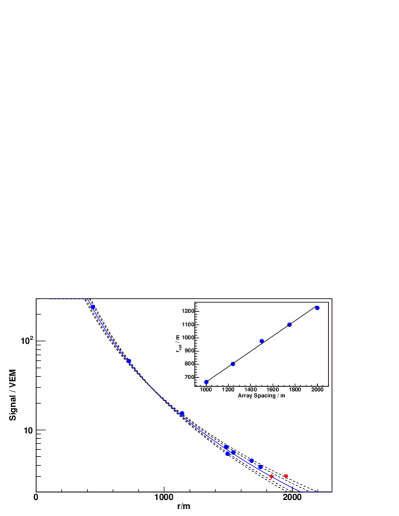
Figure 3: LDFs of an Auger SD event, analysed with different slope parameters. Red points indicate stations with zero signal. The inset shows how the optimum ground parameter $r_{opt}$ varies with the array spacing.

parameter has very little dependence on zenith angle, energy, or the form of the LDF used to reconstruct the showers. For example, an analysis of $\sim 500$ Auger SD events with energies $10^{18.5}$ eV $<E<10^{19}$ eV and zenith angles $0^{\circ}<\theta<60^{\circ}$ gives a distribution of $r_{opt}$ with mean 940 m and a rms of 110 m. An analysis of simulated events at $10^{20}$ eV gives a mean of 930 m and a rms deviation of 40 m. The prescence of a saturated station (predominantly in vertical, high energy events) tends to push $r_{opt}$ out by several hundred metres, and after an analysis of many showers, at different zenith angle and energy, S(1000) was chosen as a robust ground parameter to measure all showers at. At 1000 m from the core the mean uncertainty in $S(r)$ (across all events) is minimised, and furthermore, for the few showers where $r_{opt}$ lies far from 1000 m, the uncertainty in S(1000) can easily be estimated.

5 Summary and Outlook

The lateral distribution function of EAS observed using the Auger Observatory has been derived. Different functions have been tested and it is concluded that an NKG-like LDF describes the data well. The dependence of the function on atmospheric depth has been described. It should be emphasized that the global shower observables, like the lateral distribution of particles, are not affected by the geomagnetic field for zenith angles $\theta<70^{\circ}$. However, for the case of very inclined showers which are dominated by muons, the density at ground is rendered quite asymmetric by the geomagnetic field and the LDF approach is not longer valid [2, 7].

References

- [1] Abraham J. et al., (Auger Collaboration), Nucl. Instr. Meth. A 523 (2004) 50-95
- [2] Ave M. et al., Astropart. Phys. 14 (2000) 91
- [3] Coy R.N. et al., Astropart. Phys. 6 (1997) 263
- [4] Coy R.N. et al., Proc. 17th ICRC, Paris (1981) vol.6.
- [5] Ghia P. et al. for the Auger Collaboration, these proceedings (ita-ghia-P-abs1-he14-oral)
-
[6]
Greisen K, Progress in Cosmic Ray Physics 3 (1956) North Holland Publ.
Kamata K and Nishimura J. Prog. Theoret. Phys. Suppl. 6 (1958) 93 - [7] Hillas A.M. et al., Proc. 11th ICRC, Budapest (1969), Acta Physica Academiae Scietiarum Hungaricae 29, Suppl. 3, (1970) 533
- [8] Roth M. for the Auger Collaboration, Proc. 28th ICRC, Tsukuba (2003) 333.
- [9] Salazar H. for the Auger Collaboration, Proc. 27th ICRC, Hamburg (2001) 752.