The GRB Variability/Peak Luminosity Correlation: new results

Abstract

We report test results of the correlation between time variability and peak luminosity of Gamma-Ray Bursts (GRBs), using a larger sample (32) of GRBs with known redshift than that available to Reichart et al. (2001), and using as variability measure that introduced by these authors. The results are puzzling. Assuming an isotropic-equivalent peak luminosity, as done by Reichart et al. (2001), a correlation is still found, but it is less relevant, and inconsistent with a power law as previously reported. Assuming as peak luminosity that corrected for GRB beaming for a subset of 16 GRBs with known beaming angle, the correlation becomes little less significant.

1 Introduction

Despite the small number of Gamma-Ray Bursts (GRBs) with known redshift (several dozens), several correlations between intrinsic temporal or spectral parameters of the GRB prompt emission and GRB energetics have been discovered in the last seven years. Norris et al. (2000) found an anticorrelation between peak luminosity and the spectral lag (obtained by cross-correlating the time profiles of the same GRB in various energy bands), according to which more luminous bursts exhibit shorter lags. Salmonson & Galama (2002) discovered a positive correlation between the spectral lag of the gamma-ray prompt emission and the jet-break time of the afterglow decay, according to which a small break time corresponds to a small lag and consequently to a high peak luminosity of the GRB. Concerning the temporal properties of GRB time profiles, evidence has been found for a positive correlation between temporal variability of the light curves and isotropic-equivalent peak luminosity for the GRBs with known redshift (Reichart et al. 2001, hereafter R01; Fenimore & Ramirez-Ruiz 2000).

Moreover Reichart et al. (2003) have shown that the variability vs. peak luminosity correlation could also hold true for X-Ray Flashes (XRFs; see Heise et al. (2001)). As a consequence of the mentioned correlations, a correlation between time variability and spectral lag is also expected and confirmed for a large sample of BATSE bursts (Schaefer et al., 2001). The variability vs. peak luminosity correlation has been explained by several authors (e.g., Kobayashi et al. (2002); Mészáros et al. (2002)) mainly within the framework of the standard fireball model, according to which internal shocks between ultra relativistic shells are responsible for the pulse-like structure of the GRB prompt emission, while the smooth afterglow emission is due to external shocks between the fireball wind and the matter surrounding the GRB progenitor (e.g., Piran (2004) for a review).

GRB variability-connected properties are thought to be more sensitive to the bulk Lorentz factor $\Gamma$ and, if the GRB emission is beamed, to the jet opening angle and/or the viewing angle (e.g., Salmonson & Galama (2002); Ioka & Nakamura (2001)). Within the fireball model, there are different mechanisms that could account for different time variabilities, also giving possible explanations for XRF properties (Mészáros et al., 2002). In addition, the “cannonball model” for GRBs (Dado, Dar & De Rújula, 2002) also seems to explain the variability vs. peak luminosity correlation (Plaga, 2001).

From the above correlations also luminosity estimators have tentatively been derived (Reichart et al., 2001; Fenimore & Ramirez-Ruiz, 2000; Schaefer et al., 2001) to investigate general properties of GRBs, such as the luminosity function and the possible link with the star formation rate. In addition, empirical redshift indicators have been proposed based on the calibration derived with the small sample of GRBs with known redshift, making use of the X- and gamma-ray observations alone (Atteia, 2003; Bagoly et al., 2003).

In this work we test the variability vs. peak luminosity correlation using the variability definition given by R01. We used a sample of 32 GRBs with known redshift. Furthermore we studied the same correlation by replacing the isotropic-equivalent peak luminosity with that corrected for beaming for a subset of 16 GRBs with known collimation angle provided by Ghirlanda et al. (2004).

In Section 2, we discuss our sample of GRBs; in Section 3 we discuss the time variability analysis; in Section 4 we estimate the peak luminosity of the GRB in our sample and compare it with the R01 results. In Section 5 we present our results on variability/peak luminosity correlation, in Section 6 we discuss our results.

2 The GRB sample

2.1 GRBs with known redshift

The sample of 32 GRBs with known redshift includes 16 GRBs detected by the Gamma-Ray Burst Monitor (GRBM) (Feroci et al., 1997; Frontera et al., 1997; Costa et al., 1998) on board the BeppoSAX satellite (Boella et al., 1997) during the period 1997–2002, two by the BATSE experiment (Paciesas et al., 1999) aboard the Compton Gamma–Ray Observatory (CGRO), six by the FREGATE instrument aboard HETE-II (Atteia et al., 2003), one by Konus/WIND (Aptekar et al., 1995), one by Ulysses (Hurley et al., 1992) and six by BAT/Swift (Gehrels, 2004). Eight of the 16 GRBs detected with the BeppoSAX GRBM were also detected with BATSE. We used public archives for GRB data obtained with BATSE, HETE-II, Konus/WIND, and BAT/Swift. Table 1 reports the list of the GRBs in our sample with mentioned the spacecraft that detected it. When the same GRB has been detected by more than one instrument, we first checked the consistency of the results derived from different data sets and then concentrated on the instrument which had the best SNR.

The time binning of the GRB light curves in our sample, which was used to derive the time variability, was the following: 7.8125 ms for the GRBM data, 64 ms for BATSE, 164 ms for HETE-II, 64 ms for Konus/WIND, 31.25 ms for Ulysses. In the case of BAT/Swift we made use of the event files and extracted the mask-tagged light curves with a binning time of 8 ms. Given that for the GRBs detected with the BeppoSAX GRBM, the high-resolution (7.8125-ms binning) time profiles are available in the 40–700 keV energy band, for the others we used the light curves in the energy bands which have the largest intersection with the 40–700 keV band: 110–320 keV (channel 3) for BATSE, 30–400 keV (band C) for FREGATE, 25–100 keV for Ulysses and 50–200 keV for Konus/WIND. In order to match the GRBM band, for BAT/Swift we extracted the light curves from the event files in the 40–350 keV band.

For GRB990510, given that the 7.8125-ms GRBM light curve is not available, we preferred to use 64-ms BATSE data rather than the 1-s GRBM light curve.

Six GRBs (980613, 011211, 021004, 050126, 050318 and 050416) with known redshift were not included in our sample due to their low signal, which prevented us from deriving a statistically significant variability estimate. Another GRB (021211, detected with HETE-II) was not included in the sample, due to the high ratio between binning time and smoothing time which could bias the variability estimate (see Section 3). Other GRBs with known redshift (000301C, 000418, 000926) detected by both Konus/WIND and Ulysses were not included in our sample, because unfortunately both Konus public and Ulysses data cover their light curves only partially.

In the case of BATSE (970828 and 000131) the usual 4-channel 64-ms light curves are not available. Thus we made use of the 16-channel MER spectra acquired along either entire GRB with an integration time of 64 ms. Therefore we rebinned the 16-energy-channel MER data both spectrally and temporally in order to reproduce as much as possible the 4-channel scheme of BATSE 64-ms light profiles. As we discuss below, we relied on coarse time resolution light curves only when the overall duration of the GRB was very long compared to the binning time.

In general the data available cover the entire time profile of the GRBs in our sample. However there are some exceptions. In the case of the GRBM events, given that the high-resolution data cover 8 s before the trigger time and 98 s after it, in the case of the longest events (990506 and 010222, $T_{90}=129$ s and $T_{90}=97$ s, respectively), it is not true. In these cases, the measure of time variability was obtained summing the variability in the part covered by the 7.8125-ms bins with that in the part covered by 1-s ratemeters (the tail of the burst).

GRB000210 ($T_{90}=8.1$ s) suffers from a 2.5-s long gap due to corrupted high-resolution data occurred in the middle of the burst profile. Using the 1-s data, the mean 7.8125-ms light profile in the gap was reconstructed adding to the mean profile a Poisson noise. The value of GRB time variability so derived was found not to significantly change, even adding in the gap a non-Poisson noise compatible with the 1-s time profile.

For each GRB detected with the GRBM, we considered the light curves of the two most illuminated units and checking whether the best signal-to-noise ratio (SNR) was obtained from a single unit or by summing the two units.

We found that for the 11 GRBs detected by GRBM and Wide Field Cameras (WFCs) (Jager et al., 1997), the best signal is obtained from a single GRBM unit (that with the larger area exposed to the GRB). For the five bursts detected with the GRBM but not with the WFCs the best signal was obtained by summing the two most illuminated units: units 1 and 4 (980703), 3 and 4 (990506, 020405), 2 and 4 (991216, 010921). In principle the operation of adding the counts of different units is questionable because of dead time, as it will be discussed in Section 3. In practice, for the above cases we made sure that the results were consistent with those obtained when considering only the most illuminated unit for each GRB. This has been found to be no longer true, i.e. the correction for dead time becomes not negligible, when considering very small smoothing time-scales (Rossi et al., in preparation).

Table 1: Variability vs. Peak Luminosity for 32 GRBs with known redshift (1$\sigma$ errors).

GRB	$z$	Mission(a)	$T_{f=0.45}$	$V_{f=0.45}$	Peak Lum. $L^{\rm(b)}$	$z$ Refs.(c)
Name	Redshift		(s)		($10^{50}$ erg s-1)
970228	0.695	BS/U/K	$2.2$	$0.223_{-0.017}^{+0.018}$	$48.7\pm 9.9$	1
970508	0.835	B/BS/U/K	$2.4$	$0.023_{-0.013}^{+0.013}$	$9.43\pm 1.89$	2
970828	0.958	B/U/K/S	$12.9$	$0.101_{-0.002}^{+0.002}$	$120.0\pm 40.0$	3
971214	3.418	BS/B/U/K/N/R	$4.4$	$0.110_{-0.012}^{+0.012}$	$360.\pm 65.$	4
980425	0.0085	B/BS/U/K	$4.7$	$0.049_{-0.048}^{+0.048}$	$0.0007\pm 0.0002$	5
980703	0.966	BS/B/U/K/R	$3.2$	$0.044_{-0.007}^{+0.007}$	$26.4\pm 5.6$	6
990123	1.6	BS/B/U/K	$12.8$	$0.112_{-0.002}^{+0.002}$	$840.\pm 121.$	7
990506	1.3	BS/B/U/K/R	$8.6$	$0.270_{-0.005}^{+0.005}$	$583.\pm 121.$	8
990510	1.619	B/BS/U/K/N	$3.2$	$0.214_{-0.008}^{+0.005}$	$300.\pm 50.$	9
990705	0.86	BS/U/K/N	$8.0$	$0.178_{-0.003}^{+0.003}$	$134.\pm 21.$	10,11
990712	0.434	BS/U/K	$4.1$	$0.042_{-0.017}^{+0.017}$	$5.4\pm 1.0$	12
991208	0.706	K/U/N	$5.1$	$0.082_{-0.003}^{+0.003}$	$290.\pm 100.$	13
991216	1.02	BS/B/U/N	$2.6$	$0.193_{-0.002}^{+0.002}$	$1398.\pm 200.$	14
000131	4.5	B/U/K/N	$8.0$	$0.187_{-0.005}^{+0.005}$	$3600.\pm 900.$	15
000210	0.846	BS/U/K	$1.59$	$0.026_{-0.002}^{+0.002}$	$480.\pm 50.$	16
000911	1.058	U/K/N	$5.2$	$0.077_{-0.034}^{+0.034}$	$360.\pm 60.$	17
010222	1.477	BS/U/K	$6.62$	$0.201_{-0.003}^{+0.003}$	$801.\pm 119.$	18
010921	0.45	BS/H/U/K	$5.3$	$0.038_{-0.016}^{+0.016}$	$8.0\pm 2.0$	19
011121	0.36	BS/U/K/O	$8.3$	$0.049_{-0.002}^{+0.002}$	$19.9\pm 3.1$	20
020124	3.198	H/U/K	$8.8$	$0.203_{-0.032}^{+0.031}$	$300.\pm 60.$	21
020405	0.69	BS/U/K/O	$9.9$	$0.168_{-0.007}^{+0.007}$	$71.4\pm 11.2$	22
020813	1.25	H/U/K/O	$17.4$	$0.248_{-0.007}^{+0.007}$	$340.\pm 70.$	23
030226	1.98	H/K/O	$26.6$	$0.042_{-0.015}^{+0.015}$	$25.0\pm 5.0$	24
030328	1.52	H/U/K	$24.9$	$0.051_{-0.005}^{+0.005}$	$90.\pm 18.$	25
030329	0.168	H/U/K/O/RH	$4.9$	$0.105_{-0.007}^{+0.007}$	$6.1\pm 1.2$	26
041006	0.712	H/K/RH	$8.0$	$0.052_{-0.002}^{+0.002}$	$66.\pm 10.$	27
050315	1.949	BSw	$12.3$	$0.042_{-0.031}^{+0.032}$	$38.\pm 8.$	28
050319	3.24	BSw	$3.6$	$0.061_{-0.030}^{+0.032}$	$84.\pm 20.$	29
050401	2.90	BSw	$4.4$	$0.195_{-0.029}^{+0.028}$	$740.\pm 100.$	30
050505	4.27	BSw	$9.0$	$0.205_{-0.044}^{+0.043}$	$250.\pm 50.$	31
050525	0.606	BSw	$2.0$	$0.111_{-0.003}^{+0.003}$	$80.\pm 10.$	32
050603	2.821	BSw	$1.2$	$0.245_{-0.034}^{+0.037}$	$1200.\pm 200.$	33

• Mission: BS (BeppoSAX), B (BATSE/CGRO), K (Konus/WIND), H (HETE-II), U (Ulysses), S (SROSS-C), N (NEAR), R (RossiXTE), O (Mars Odyssey), RH (RHESSI), BSw (BAT/Swift): the data used are taken from the first mission mentioned.

• Isotropic-equivalent peak luminosity in $10^{50}$ erg s^-1 in the rest-frame 100–1000 keV band, for peak fluxes measured on a 1-s time-scale, $H_{0}=65$ km s^-1 Mpc^-1, $\Omega_{m}=0.3$, and $\Omega_{\Lambda}=0.7$.

• References for the redshift measurements: (1) Djorgovski et al. (1999), (2) Metzger et al. (1997), (3) Djorgovski et al. (2001a), (4) Kulkarni et al. (1998), (5) Tinney et al. (1998), (6) Djorgovski et al. (1998), (7) Kulkarni et al. (1999), (8) Bloom et al. (2003), (9) Beuermann et al. (1999), (10) Amati et al. (2000), (11) Le Floc’h et al. (2002), (12) Galama et al. (1999), (13) Dodonov et al. (1999), (14) Vreeswijk et al. (1999), (15) Andersen et al. (2000), (16) Piro et al. (2002), (17) Price et al. (2002a), (18) Garnavich et al. (2001), (19) Djorgovski et al. (2001b), (20) Infante et al. (2001), (21) Hjorth et al. (2003), (22) Masetti et al. (2002), (23) Price et al. (2002b), (24) Greiner et al. (2003a), (25) Martini et al. (2003), (26) Greiner et al. (2003b), (27) Fugazza et al. (2004), (28) Kelson & Berger (2005), (29) Fynbo et al. (2005a), (30) Fynbo et al. (2005b), (31) Berger et al. (2005), (32) Foley et al. (2005), (33) Berger & Becker (2005).

As far as the 8 bursts detected with both GRBM and BATSE (970508, 971214, 980425, 980703, 990123, 990506, 990510, 991216) are concerned, we used the BeppoSAX data for 971214, 980703, 990123, 990506, and 991216, for which the higher time resolution of the GRBM turned out to be essential for a better variability estimate, while for the remaining 3 GRBs (970508, 980425, and 990510) we used the BATSE data given the better SNR, after verifying the mutual consistency of the GRBM and BATSE variability results.

3 Variability measure

We adopted the variability measure given by R01, slightly modified for two corrections which could affect the result: the instrument dead time, and a small non-Poisson noise present in the GRBM background data. The variability measure used by R01 was defined as a properly normalised mean square deviation of the intrinsic light curve of a GRB in a given energy band from a smoothed one. For a discrete light curve made of N bins, the variability measure, according to R01, is given by:

$$~{}~{}~{}~{}~{}~{}~{}V_{f,P} = \frac{\sum_{i=1}^{N}[S_{i}(C_{j},N_{z})-S_{i}(C_{j},N_{f})]^{2}}{\sum_{i=1}^{N}[S_{i}(C_{j},N_{z})-B_{i}]^{2}},$$ (1)

where as intrinsic light curve we mean the GRB light curve in the source-frame, $N_{f}$ is the number of data bins corresponding to the smoothing time scale $T_{f}$ defined by R01 as the shortest cumulative time interval during which a fraction $f$ of the total counts above background has been collected, $C_{j}$ and $B_{i}$ are the original GRB (source plus background) and background counts in the bins $j$ and $i$, respectively, in the observer frame, the index $P$ means that the variability measure is inclusive of the Poisson noise. $S_{i}(C_{j},N_{x})$ is roughly the mean counts on $N_{x}$ bins ($x=z$ or $f$) centred around the $i$-th bin:

$$S_{i}(C_{j},N_{x})=\frac{1}{N_{x}}\big{[}\sum_{j=i-n_{x}}^{i+n_{x}}C_{j}+~{}~{}~{}~{}~{}~{}~{}~{}~{}~{}~{}~{}~{}~{}~{}~{}~{}~{}~{}~{}~{}~{}~{}$$

$$~{}~{}~{}~{}~{}~{}~{}~{}~{}~{}~{}~{}~{}~{}~{}~{}~{}~{}~{}~{}~{}~{}+\big{(}\frac{N_{x}-1}{2}-n_{x}\big{)}\ (C_{i-n_{x}-1}+C_{i+n_{x}+1})\big{]}.$$ (2)

$N_{z}$ is the number of bins in the observer-frame, which corresponds to 1 bin in the source-frame. Assuming as time duration of 1 bin in the source-frame the shortest binning $\Delta t$ of the data (e.g., in the case of the BeppoSAX GRBM, $\Delta t=7.8125$ ms), in the observer-frame the number of bins, depending on the GRB redshift $z$, for relativistic time dilation and narrowing of the light curves at high energies (Fenimore et al., 1995), is given by $N_{z}=(1+z)^{\beta}$ with $\beta\approx 0.6$. Thus $N_{z}$ can take values other than integers and $n_{x}$ is the truncated integer value of $(N_{x}-1)/2$.

R01 found that the best luminosity estimator is obtained when using $f=0.45$; for this reason, we fixed $f=0.45$.

The variability $V_{f,P}$ can also be written as follows:

$$~{}~{}~{}~{}~{}~{}~{}V_{x,P} = \frac{\sum_{i=1}^{N}(\sum_{j=1}^{N}a_{ij}C_{j})^{2}}{\sum_{i=1}^{N}(\sum_{j=1}^{N}b_{ij}C_{j}-B_{i})^{2}}$$ (3)

where the coefficients $a_{ij}$ and $b_{ij}$, for each GRB, are computed by comparing eq. 3 with eq. 1 through eq. 3.

Following R01, after subtraction of the Poisson variance the variability measure is given by

$$V_{f}=\frac{\sum_{i=1}^{N}[(\sum_{j=1}^{N}a_{ij}C_{j})^{2}-\sum_{j=1}^{N}a_{ij}^{2}\,C_{j}]}{\sum_{i=1}^{N}[(\sum_{j=1}^{N}b_{ij}C_{j}-B_{i})^{2}-\sum_{j=1}^{N}b_{ij}^{2}\,C_{j}]}$$ (4)

which is the expression used by R01 to evaluate the variability of the GRBs in their sample. We slightly modified the above expression by taking also into account the dead time, which is known to affect the Poisson variance of a stationary process (Müller, 1973, 1974; Libert, 1978). In the case of a stationary Poisson process with measured mean rate $\mu$, the variance of its counts in the time bin $\Delta t$, which is given by $\mu\Delta t$ in absence of dead time, becomes $\mu\Delta t\ (1-\mu\tau)^{2}$ in the asymptotic limit $\tau/\Delta t\ll 1$, where $\tau$ is the dead time. In the case of the BeppoSAX GRBM $\tau=4\mu$s, $\tau/\Delta t\simeq 5\times 10^{-4}$ for the shortest bin duration $\Delta t=7.8125$ ms. In the same limit $\tau/\Delta t\ll 1$, the same correction factor $(1-\mu\tau)^{2}$ applies to the white noise level of the power spectral density (PSD) estimate (Frontera & Fuligni, 1978; van der Klis, 1989). It is shown (Frontera & Fuligni, 1979) that the same correction factor holds when the process is non-stationary, like GRBs or flares. Potentially our variability calculations could be sensitive to dead time, especially for those GRBs with huge peak count rates, like in the case of 990123 ($\sim$16,000 cts/s with GRBM), for which, around the peak, the true variance is $\sim 0.9$ times the measured counts.

In addition, we corrected for a slight (a few percent) non-Poisson noise found in the GRBM high-resolution data. This noise increases the Poisson variance by a factor $r_{np}$ which ranges from 1.027 to 1.049, depending on the detection unit, for the GRBM data after November 1996 .

Taking into account both dead time and non-Poisson noise, the right terms to be subtracted in the numerator and denominator of eq. 3 become $\sum_{j=1}^{N}a_{ij}^{2}C_{j}\ r_{j}$ and $\sum_{j=1}^{N}b_{ij}^{2}C_{j}\ r_{j}$, respectively (see, for comparison, eq. 4), where

$$r_{j}=r_{np}\ \big{(}1-C_{j}\,\frac{\tau}{\Delta\,t}\big{)}^{2}$$ (5)

As a consequence, the expression we used to estimate the net GRB time variability is given by:

$$V_{f}=\frac{\sum_{i=1}^{N}[(\sum_{j=1}^{N}a_{ij}C_{j})^{2}-\sum_{j=1}^{N}a_{ij}^{2}\,C_{j}\,r_{j}]}{\sum_{i=1}^{N}[(\sum_{j=1}^{N}b_{ij}C_{j}-B_{i})^{2}-\sum_{j=1}^{N}b_{ij}^{2}\,C_{j}\,r_{j}]}$$ (6)

We used as statistical uncertainty $\sigma_{V_{f}}$ on the variability measure that given by R01 (eq. 8) properly modified to take into account the correction factor $r_{j}$.

We found that the variability measure is not sensitive to dead time corrections for long GRBs, in which $T_{f=0.45}$ is much longer than the bin time, while it is significantly modified for relatively short GRBs exhibiting sharp intense pulses.

3.1 Variability dependence on binning time

In order to understand how time binning affects the GRB variability, for the brightest GRBs, detected with either GRBM or BATSE we evaluated the variability measure (eq. 6) as a function of the binning time of the data. The result is that the variability is better estimated for very short time durations of the data bins with respect to the smoothing time-scale $T_{s}=T_{f=0.45}$. More specifically, it results that the variability significantly decreases for few 0.01$<\Delta\,t/T_{s}<$ few 0.1, and becomes unreliable when this ratio becomes still higher, i.e. for $\Delta\,t/T_{s}>$few 0.1.

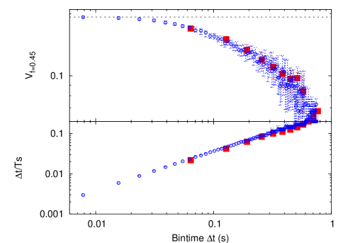
Figure 1: Top panel: Variability of 991216 as a function of binning time $\Delta t$ using both GRBM (blue circles) and BATSE (red squares) data sets. Black dotted line represents the asymptotic value of $V_{f=0.45}$ as derived with GRBM data using small binning times. Also shown is the ratio between binning time and smoothing time-scale (bottom panel).

On the other side, the bin time should be long enough to collect a good number of photons (typically at least 20 per bin on average) to ensure the Gaussian limit and take over the effects of statistical fluctuations. Thus we rejected those GRBs whose data sets do not match the above requirements.

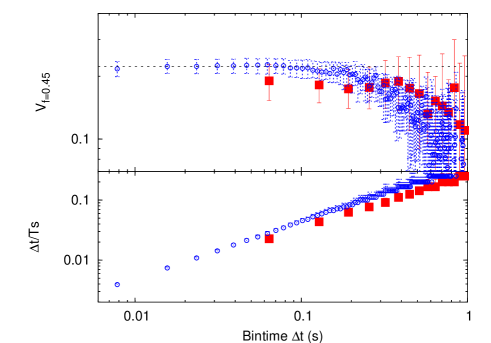
Figure 2: Top panel: Variability of 970228 as a function of binning time $\Delta t$ using both GRBM (blue circles) and KONUS (red squares) data sets. Black dotted line represents the asymptotic value of $V_{f=0.45}$ as derived with GRBM data using small binning times. Also shown is the ratio between binning time and smoothing time-scale (bottom panel).

Figures 1 and 2 show the illustrative cases of 991216 and 970228, respectively. We calculated $V_{f=0.45}$ using both GRBM and BATSE (KONUS) data sets as a function of the binning time for 991216 (970228). For both GRBs, the variability seems to approach an asymptotic value for decreasing values of binning time. In the case of 991216, it appears that the original binning time of BATSE, 64 ms, is a little too coarse since its correspondent value of $V_{f=0.45}$ is significantly lower: we assume as asymptotic value the measure obtained with the smallest binning time of GRBM data and get $V_{f=0.45}=0.193\pm 0.002$, while the BATSE measure is $0.170\pm 0.003$, i.e. $\sim$6-$\sigma$ apart. Differently, in the case of 970228 the KONUS measure with the smallest binning time of 64 ms yields a measure of $V_{f=0.45}$ which is apparently consistent with the GRBM one (Fig. 2). In the case of 991216 it is worth noting that the measure of $V_{f=0.45}$ turns out to be significantly underestimated with respect to the asymptotic value as far as we assume binning times at least a few $10^{-2}$ times as high as the smoothing time-scale.

In general, we noticed that for all the GRBs for which $V_{f=0.45}$ approaches an asymptotic value for small binning times, different measures of $V_{f=0.45}$ are still consistent with that, provided that the ratio between binning time and smoothing time-scale is not too high ($\Delta t/T_{s}<$ few $10^{-2}$).

Our final set of variability measures include only those GRBs for which the three following requirements have been fulfilled with a single binning time: 1) smallness of ratio $\Delta t/T_{s}$, 2) asymptotic behaviour of $V_{f=0.45}$ as a function of binning time $\Delta t$ for small $\Delta t$, 3) Gaussian limit of at least 20 counts per bin on average.

Following this guideline, we discarded the HETE-II bursts 021211 and 050408, for which $\Delta\,t/T_{s}$ is around 0.2 and 0.08, respectively. In the case of the couple of GRBs above considered, we infer that GRBM data turned out to be essential in estimating the variability of 991216, since BATSE data alone, although consistent with GRBM data for comparable binning times, do not seem to approach an asymptotic value of $V_{f=0.45}$, while GRBM data do. On the other side, in the case of 970228 KONUS data exhibit an asymptotic trend towards small binning times; together with the fulfillment of the other two requirements, KONUS time resolution is acceptable and yields a variability measure which is consistent with the GRBM within errors.

4 Peak Luminosity Estimate

The GRBs peak luminosities were estimated using the definition of luminosity distance in the source-frame 100–1000 keV energy band:

$$L\ =\ 4\pi D_{L}^{2}(z)\ \int_{100/(1+z)}^{1000/(1+z)}E\Phi(E)\,dE$$ (7)

where $\Phi(E)$ is the measured spectrum (ph cm^-2s^-1keV^-1) around the peak time, $D_{L}(z)$ is the luminosity distance at redshift $z$, $E$ is energy expressed in keV. By replacing $E^{\prime}=E(1+z)$ we get:

$$L\ =\ \frac{4\pi D_{L}^{2}(z)}{(1+z)^{2}}\ \int_{100}^{1000}{E^{\prime}\Phi\Big{(}\frac{E^{\prime}}{1+z}\Big{)}\,dE^{\prime}}$$ (8)

Formally, eq. 8 is the same as eq. 9 of R01: there $D(z)$ is the co-moving distance, which is equal to $D(z)=D_{L}/(1+z)$ if we consider a flat Universe. However, unlike R01 who used as $\Phi(E)$ the best-fitting Band model (Band et al., 1993) to the average GRB count spectrum normalised to the peak count rate, we used for the GRBM data the best-fitting power-law spectrum ($\Phi(E)=NE^{-\alpha}$) to the GRB peak count rate spectrum obtained from the 1-s ratemeters available in two channels (40–700 keV and $>100$ keV). When the 225-channel time-averaged spectrum was not available, we added a conservative 10% systematics to the peak luminosity uncertainties. Thus, for the GRBM bursts, eq. 8 becomes:

$$L\ =\ 4\pi D_{L}^{2}(z)\ (1+z)^{\alpha-2}\,F_{p}$$ (9)

where $F_{p}=\int_{100}^{1000}NE^{\prime 1-\alpha}dE^{\prime}$ is the 100–1000 keV peak flux measured in the observer frame (erg cm^-2s^-1).

Figure 3: Peak luminosity $L_{\textrm{GRBM}}$ derived with GRBM data vs. peak luminosity $L_{\textrm{R01}}$ published by Reichart et al. using data from BATSE, Konus/WIND and Ulysses, for a common sample of GRBs. The dashed line shows the equation $L_{\textrm{R01}}=L_{\textrm{GRBM}}$. See text.

In the case of GRBs with sharp peaks of $<1$ s duration (e.g. GRB000214), the peak luminosity obtained from 1-s ratemeters was further corrected by the ratio between the actual peak value and that derived from 1-s ratemeters.

For the GRBs in our sample not detected with the GRBM, we used the best-fitting parameters of $\Phi(E)$ available from the literature. The best-fitting spectral parameters for HETE-II bursts were taken from Sakamoto et al. (2004), except for the recent 041006 for which we used the best-fitting cutoff power-law parameters published by HETE-II team on the HETE web page ($E_{\rm 0}$=100.2 keV, $\alpha=1.367$). For the Ulysses GRB000911 we made use of the best-fitting parameters published by Price et al. (2002a), while for the Konus burst 991208 we used the parameter values given by R01. For the BATSE GRB000131 we fitted the peak energy spectrum from MER data in the range 30–1000 keV with the Band function ($\alpha=-0.56$, $\beta=-2.17$, $E_{0}=153$ keV, $\chi^{2}/{\rm dof}=1.0$). Likewise, for the BATSE GRB970828 the peak energy spectrum was fitted with the Band function ($\alpha=-0.65$, $\beta=-2.56$, $E_{0}=269$ keV, $\chi^{2}/{\rm dof}=1.1$). For BAT/Swift we extracted from the event file the 1-s 80-channel spectrum around the peak; for all the 6 BAT/Swift GRBs considered, the peak spectrum was fitted with a simple power law in the 15-350 keV range, apart from a couple of them (050525 and 050603) for which only the cut-off power-law model yields a good fit. We then used eq. 7 to evaluate the peak luminosity.

Our peak luminosity estimates are reported in Tables 1.

For the common sample of GRBs, our estimates of the peak luminosity are fully consistent with those obtained by R01 (see Fig. 3).

5 Results

5.1 GRBs with known redshift

First of all we evaluated the time variability of the GRBs (13) common to our sample and to that by R01, in order to test the mutual consistency of our results with those obtained by R01.

5.1.1 Variability

Figure 4 compares the two time variability estimates. As can be seen, the results are well consistent with each other, except for three cases (970228, 991216, and 000131).

Figure 4: Variability according to R01’s definition derived in this paper vs. Variability published by R01 for a common sample of 13 GRBs. The dashed line shows the equation corresponding to equality. See text.

For each of these GRBs we investigated the reason of the discrepant measure of $V_{f=0.45}$ first of all by trying to reproduce the results by R01 using KONUS data alone for 970228 and BATSE data alone for the other two.

5.1.2 GRB 970228

In order to reproduce R01’s results for 970228 we used the same data set, i.e. the light curve by KONUS. The only difference is that we used public data that include a single light curve in the 50–200 keV energy band, while R01 used three different energy bands: 10–45 keV, 45–190 keV and 190–770 keV. R01 report the smoothing time-scale for each of the three energy channels and only the global variability measure derived from merging the three different measures according to the procedure described therein. Our measure of the smoothing time-scale is $2.82\pm 0.32$ s to be compared with that obtained by R01 for the same energy channel, i.e. 2.891 s (no error is reported), thus consistent. Our variability measure with KONUS data is $0.19\pm 0.04$ to be compared with R01’s one, $0.08\pm 0.05$. The measure obtained with GRBM data, $0.22\pm 0.02$, well agrees with our KONUS measure (see Fig. 2), but does not with R01 KONUS one. The measure reported by R01 was derived from the three energy channels; this might partially explain the difference. However, we notice that our KONUS measure is 2.2-$\sigma$ apart from the R01 value of $0.08$. We are led to think of two potential sources of discrepancy between our measure and R01’s. First, the overall time interval containing the GRB might be different; second, the extrinsic scatter that R01 find on the global measure of $V_{f=0.45}$ is a little underestimated with respect to what we find comparing a single KONUS channel with the R01 global measure. We address the reader to the R01 paper for a definition of the extrinsic scatter of variability due to the different energy channels derived for each GRB. Since we neither have the same KONUS data as R01, nor we know the overall time interval adopted by R01, we cannot establish conclusively the reason for the discrepancy for this GRB. However, concerning the first possibility, we tentatively adopted other time intervals trying to match the variability measure reported by R01. We find a variability measure of $0.08\pm 0.03$ for a time interval including the first sharp pulse and lasting about 40 s until the first pulse following a quiescent interval from the very first pulse. It must be pointed out that our true measure was performed on a 80-s long interval, since there is evidence for emission. This could be a hint for the possible explanation of the discrepancy.

5.1.3 GRB 991216

For this GRB we adopted the measure obtained with GRBM data and we already discussed the reasons in Sec. 3.1. Here we try to reproduce the R01 results using the same BATSE data and then compare our variability measures on each energy channel with the merged value derived by R01.

Figure 5: Variability of 991216 as derived with BATSE data as a function of the energy channel. Dashed lines show the merged value $\pm 1~{}\sigma$ obtained by R01.

In Figure 5 we show the variability as a function of the BATSE energy channel and compare them with the merged value $\pm 1~{}\sigma$ reported by R01. We remind that when comparing with GRBM results, we just considered channel 3. In particular for this GRB, we know from previous discussion that the value obtained with BATSE channel 3 appears to be underestimated with respect to the GRBM result (see Fig. 1).

We have a perfect match within errors between our set of four smoothing time-scale values and those obtained by R01. Therefore we are led to conclude that our variability measures should match consequently. On this basis, from Fig. 5 we notice that the extrinsic scatter by R01, whose 1-$\sigma$ region is displayed through dashed lines, seems to be little underestimated. In fact, the channel 1 measure is 2.6-$\sigma$ below and the channel 3 is 3-$\sigma$ above. In addition to this, we remind that for this particular GRB exhibiting sharp pulses we know from GRBM data that a time binning of 64 ms is too coarse (see Fig. 1 and discussion in Sec. 3.1). We therefore conclude that the effect of a higher scatter of variability at different energy channels than that estimated by R01, combined with the fact the for this GRB a binning time of 64 ms seems inadequate, account for the discrepancy between our measure of variability for 991216 and that published by R01.

5.1.4 GRB 000131

For this GRB we made use of BATSE data while R01 used KONUS data. Unfortunately the public KONUS data of this GRB do not cover the whole profile, so we are bound to use BATSE data alone and compare our variability measures with the R01 value. Figure 6 displays the variability as a function of the BATSE energy channel and dashed lines show the R01 estimate.

Figure 6: Variability of 000131 as derived with BATSE data as a function of the energy channel. Dashed lines show the merged value $\pm 1~{}\sigma$ obtained by R01 with KONUS data.

The reasons of the discrepancy, which is apparent from Fig. 6, are due to the different smoothing time-scales: by comparing our set of four values with the three ones corresponding to the three lower KONUS channels (the light curve of channel 4 cannot be used according to R01), our values are systematically greater than R01’s. If we adopt the same time-scales obtained by R01 we get variability measures which are consistent within the scatter with the R01 value. This conclusively proves that the discrepancy for this GRB must be ascribed to the different measures of the time-scales. Concerning the origin of this discrepancy in the time-scales evaluation, we do not find any apparent bias that could have affected the calculations using BATSE profiles.

5.1.5 GRB 050315: a BAT/Swift GRB

The variability measured for this BAT/Swift GRB is consistent with that published by Donaghy et al. (2005). Here we want to show the consistency of the variability measure with BAT/Swift data as well as its dependence on the the different BAT energy channels. Figure 7 shows the variability as a function of the BAT channels obtained by us (asterisks and solid lines) and by Donaghy et al. (2005) (squares and dashed lines).

Figure 7: Variability of 050315 as derived with BAT/Swift data as a function of the energy channel. Asterisks and solid lines show our measures, while squares and dashed lines show the measures by Donaghy et al. (2005).

The energy bands of the three BAT channels considered are the following: 15–25 keV, 25–50 keV and 50–100 keV, respectively. Channel 5 in Fig. 7 corresponds to the integrated band 15–100 keV. These energy channels have been chosen in order to match those used by Donaghy et al. (2005). Clearly the two sets of variability measures are consistent within errors for each single BAT channels.

5.1.6 Variability/Peak Luminosity

Figure 8 and Table 1 show the $V_{f=0.45}$ vs. Peak Luminosity for the entire sample of 32 GRBs with known redshift. Dashed lines show the best-fitting power-law relationship found by R01 along with the $\pm 1\sigma$ width, according to which $L\propto V_{{\rm R01}}^{m}$, where $m=3.3_{-0.9}^{+1.1}$.

Figure 8: $V_{f=0.45}$ vs. Peak Luminosity for GRBs with known redshift. Dashed lines mark the best-fitting power-law relationship found by R01 (central line) and $\pm 1\sigma$ widths.

Apparently, from Fig. 8, the correlation between the GRB variability and the peak luminosity is confirmed, as also demonstrated by the correlation coefficients and their statistical significance. The results are given in Table 2, where we report the values of both the Pearson linear correlation coefficient $r$, and the non-parametric correlation coefficients $r_{s}$ (Spearman rank-order coefficient) and $\tau$ (Kendall coefficient) (Press et al., 1993), along with the corresponding correlation statistical significance. The same correlation coefficients have been evaluated also taking into account error bars on both $V_{f=0.45}$ and $L$ through simulations (reported among brackets in Table 2). We scattered each point along with its error bars assuming a Gaussian probability distribution in both dimensions and then we calculated the mode for each coefficient distribution.

Table 2: Correlation Coefficients for GRBs with known redshift. We also report among brackets the mode values obtained from simulations.

Kind	Coefficient	Probability
Pearson’s $r$	0.514 (0.412)	0.0026 (0.019)
Spearman’s $r_{s}$	0.625 (0.612)	0.0001 (0.0002)
Kendall’s $\tau$	0.446 (0.436)	0.0003 (0.0005)

However the high spread of the data points, clustered in two main regions of the parameter space, shows that not only the best-fitting power-law parameters obtained by R01 are in disagreement with the our results but also that a power-law model gives a bad description of the data. Indeed by fitting the data with a power-law model:

$$\log{L_{50}}\ =\ m\,\log{V_{f=0.45}}\ +\ q$$ (10)

where the peak luminosity is $L=L_{50}\times 10^{50}$erg cm^-2s^-1, independently of the method used for the fit (usual least-square fit or minimization of absolute deviations, see Press et al. (1993)), we find unsatisfactory results ($\chi^{2}>1000$, 30 dof, in either cases). Just to compare our best-fitting power-law model results with those obtained by R01, in Table 3 we report the best-fitting parameters of the power-law for the two fit methods above mentioned. In Fig. 9 we report the $1\sigma$ contour plot of the best-fitting parameters $m$ and $q$. As can be seen, the two parameters are highly correlated.

Figure 9: Contour plot of the 1$\sigma$ region of the two best-fitting parameters $m$ and $q$ (least-square fit) in the case of $V_{f=0.45}$-$L$.

Table 3: best-fitting power-law parameters of the $L$ vs. $V_{f=0.45}$ correlation for GRBs with known redshift.

Method	$m$	$q$	$\chi^{2}/{\rm dof}$
Least-square fit	$1.30_{-0.44}^{+0.84}$	$3.36_{-0.43}^{+0.89}$	1167/30
Least-absolute-deviation fit	$1.16_{-0.17}^{+0.53}$	$3.32_{-0.15}^{+0.49}$	1145/30

We also evaluated the statistical uncertainty in the $\log{L_{50}}$ as a function of $V_{f=0.45}$, taking into account the correlation between the two parameters. In Fig. 8 the point corresponding to GRB 980425 is out of the plot window to avoid scale compression, but its variability is affected by a large uncertainty ($0.049_{-0.048}^{+0.048}$) (see Table 1).

5.2 Luminosity correction for GRB beaming

For the GRBs with known redshift, we also investigated the correlation between variability $V_{f=0.45}$ and peak luminosity after correcting the luminosity values given in Table 1 for the GRB beaming angles estimated by Ghirlanda et al. (2004) . Ghirlanda et al. (2004) demonstrated that after this correction, the correlation between the peak energy $E_{\rm p}^{{\rm rest}}$ in the source frame and $E_{{\rm rad},\gamma}$ (corrected for beaming) improved with a lower spread of the data point around the best-fitting curve. From our sample of GRBs with known redshift, we considered those for which Ghirlanda et al. (2004) provided the beaming angles: the resulting subset includes 16 GRBs. In our case the result is shown in Fig. 10. Unlike the findings by Ghirlanda et al. (2004) for the Amati et al. (2002) relation, in the present case the spread of the data points becomes larger when the energy released in the GRB is corrected for beaming, although the correlation remains significant within 1%. We computed the correlation coefficients for this subset of GRBs in both cases: either assuming beaming-corrected $L_{{\rm p},\gamma}$ and isotropic equivalent $L_{\rm p}$ peak luminosities vs. variability (see Table 4).

Figure 10: Top Panel: Beaming-corrected rest-frame Peak Luminosity $L_{{\rm p},\gamma}$ vs. Variability for a subset of 16 GRBs with known redshift and beaming angle (Ghirlanda et al., 2004). Also shown are two lower limits (971214 and 011121) and three upper limits (000131, 000911 and 010921). Bottom Panel: $L_{\rm p}$ isotropic-equivalent Peak Luminosity vs. Variability for the same 16 GRBs.

Table 4: Correlation Coefficients for 16 GRBs with known redshift and beaming angle: $V$ vs. beaming-corrected $L_{{\rm p},\gamma}$ (first two columns) and $V$ vs. isotropic-equivalent $L_{\rm p}$ (last two columns).

Kind	$V$ vs. $L_{{\rm p},\gamma}$		$V$ vs. $L_{\rm p}$
	Coeff.	Prob.	Coeff.	Prob.
Pearson’s $r$	0.664	0.005	0.688	0.003
Spearman’s $r_{s}$	0.653	0.006	0.773	0.0005
Kendall’s $\tau$	0.467	0.012	0.577	0.002

As reported in Table 4 and clearly shown by Fig. 10, in the case of the isotropic-equivalent peak luminosity the spread is smaller than in the case when the correction for beaming is applied.

6 Discussion

The results found are puzzling. We confirm the peak luminosity vs. variability correlation found by R01 when we use their sample of GRBs, but we find a much larger spread of the data points when a larger sample (32 events) of GRBs is used. In this case the correlation between $V_{f=0.45}$ and $L$ is confirmed (significance $\leq$3$\times 10^{-4}$ according to non-parametric tests), but the data points are spread out in only two regions of the parameter space, with a bad description of the data points ($\chi^{2}>1000$, 30 dof) with a power-law function, which was the best-fitting function found by R01. If, in spite of that, this function is used as fit model, the power-law index derived from our data ($m=1.3_{-0.4}^{+0.8}$) is much lower than that found by R01 ($m=3.3_{-0.9}^{+1.1}$) and inconsistent with it. The correlation becomes less significant (see the comparison between the two sets of correlation coefficients in Table 4) when we correct the isotropic-equivalent peak luminosity for the GRB beaming, in contrast with the result found by Ghirlanda et al. (2004) who find a lower spread of the Amati et al. (2002) relationship when they perform this correction.

7 Conclusions

We have tested the correlation found by R01 between peak luminosity and time variability following the same method used by R01 with a larger sample of GRBs. For 32 GRBs with known redshift we confirm the existence of a correlation between the measure of time variability defined by R01 and the isotropic-equivalent peak luminosity. However we find a much higher spread of the data points in the parameter space, with the consequence that the correlation cannot be described by a power-law function as found by R01. If, in spite of that, we fit the data with this function we find that the power-law index ($1.3^{+0.8}_{-0.4}$) is much lower and inconsistent with that found by R01 ($3.3^{+1.1}_{-0.9}$). If we correct the peak luminosity for the GRB beaming, the correlation is less significant.

References

- Amati et al. (2000) Amati L. et al., 2000, Sci, 290, 953
- Amati et al. (2002) Amati L. et al., 2002, A&A, 390, 81
- Andersen et al. (2000) Andersen M.I. et al., 2000, A&A, 364, L54
- Aptekar et al. (1995) Aptekar R.L. et al., 1995, Space Sci. Rev., 71, 265
- Atteia (2003) Atteia J.-L., 2003, A&A, 407, L1
- Atteia et al. (2003) Atteia J.-L. et al., 2003, AIP Conf. Ser. Vol. 662, A Workshop Celebrating the First Year of the HETE Mission, p. 17
- Bagoly et al. (2003) Bagoly Z., Csabai I., Mészáros A., Mészáros P., Horváth I., Balázs L.G., Vavrek R., 2003, A&A, 398, 919
- Band et al. (1993) Band D. et al., 1993, ApJ, 413, 281
- Berger et al. (2005) Berger E., Bradley Cenko S., Steidel C., Reddy N., Fox D.B., 2005, GCN 3368
- Berger & Becker (2005) Berger E. & Becker G., 2005, GCN 3520
- Beuermann et al. (1999) Beuermann K. et al., 1999, A&A, 352, L26
- Bloom et al. (2003) Bloom J.S., Berger E., Kulkarni S.R., Djorgovski S.G., Frail D.A., 2003, AJ, 125, 999
- Boella et al. (1997) Boella G., Butler R.C., Perola G.C., Piro L., Scarsi L., Bleeker, 1997, A&AS, 122, 299
- Costa et al. (1998) Costa E. et al., 1998, Adv.Sp.Res., 22, 1129
- Dado, Dar & De Rújula (2002) Dado S., Dar A., De Rújula A., 2002, A&A, 388, 1079
- Djorgovski et al. (1998) Djorgovski S.G., Kulkarni S.R., Bloom J.S., Goodrich R., Frail D.A., Piro L., Palazzi E., 1998, ApJ, 508, L17
- Djorgovski et al. (1999) Djorgovski S.G., Kulkarni S.R., Bloom J.S., Frail D.A., 1999, GCN 289
- Djorgovski et al. (2001a) Djorgovski S.G., Frail D.A., Kulkarni S.R., Bloom J.S., Odewahn S.C., Diercks A., 2001a, ApJ, 562, 654
- Djorgovski et al. (2001b) Djorgovski S.G. et al., 2001b, GCN 1108
- Dodonov et al. (1999) Dodonov S.N., Afanasiev V.L., Sokolov V.V., Moiseev A.V., Castro-Tirado A.J., 1999, GCN 475
- Donaghy et al. (2005) Donaghy T.Q. et al., 2005, GCN 3128
- Fenimore et al. (1995) Fenimore E.E., In ’t Zand J.J.M., Norris J.P., Bonnell J.T., & Nemiroff R.J. 1995, ApJ, 448, L101
- Fenimore & Ramirez-Ruiz (2000) Fenimore E.E., Ramirez-Ruiz E., 2000, preprint (astro-ph/0004176)
- Feroci et al. (1997) Feroci M. et al., 1997, SPIE Conf. Ser. Vol. 3114, p. 186
- Foley et al. (2005) Foley R.J., Chen H.-W., Bloom J., Prochaska J.X., 2005, GCN 3483
- Frontera & Fuligni (1978) Frontera F., Fuligni F., 1978, Nucl. Instr. Meth., 157, 557
- Frontera & Fuligni (1979) Frontera F., Fuligni F., 1979, ApJ, 232, 590
- Frontera et al. (1997) Frontera F. et al., 1997, A&AS, 122, 357
- Fugazza et al. (2004) Fugazza D. et al., 2004, GCN 2782
- Fynbo et al. (2005a) Fynbo J.P.U., Hjorth J., Jensen B.L., Jakobsson P., Moller P., 2005a, GCN 3136
- Fynbo et al. (2005b) Fynbo J.P.U. et al., 2005b, GCN 3176
- Galama et al. (1999) Galama T.J. et al., 1999, GCN 388
- Garnavich et al. (2001) Garnavich P.M., Pahre M.A., Jha S., Calkins M., Stanek K.Z., McDowell J., Kilgard R., 2001, GCN 965
- Gehrels (2004) Gehrels N. et al., 2004, ApJ, 611, 1005
- Ghirlanda et al. (2004) Ghirlanda G., Ghisellini G., Lazzati D., 2004, ApJ, 616, 331.
- Greiner et al. (2003a) Greiner J., Günther E., Klose S., Schwarz R., 2003a, GCN 1886
- Greiner et al. (2003b) Greiner J., Peimbert M., Estaban C., Kaufer A., Vreeswijk P., Smoke J., Klose S., Reimer O., 2003b, GCN 2020
- Heise et al. (2001) Heise J., in ’t Zand J.J.M., Kippen R.M., Woods P.M., 2001, in Costa E., Frontera F., Hjorth J., eds, Proc. 2nd Rome Workshop, Gamma Ray Bursts in the Afterglow Era, Springer-Verlag, Berlin, p. 16
- Hjorth et al. (2003) Hjorth J. et al., 2003, ApJ, 597, 699
- Hurley et al. (1992) Hurley K. et al., 1992, A&AS, 92(2), 401
- Infante et al. (2001) Infante L., Garnavich P.M., Stanek K.Z., Wyrzykowski L., 2001, GCN 1152
- Ioka & Nakamura (2001) Ioka K., Nakamura T., 2001, ApJ, 554, L163
- Jager et al. (1997) Jager R. et al., 1997, A&AS, 125, 557
- Kelson & Berger (2005) Kelson D. & Berger E., 2005, GCN 3101
- Kobayashi et al. (2002) Kobayashi S., Ryde F., MacFadyen A., 2002, ApJ, 577, 302
- Kulkarni et al. (1998) Kulkarni S.R. et al., 1998, Nature, 393, 35
- Kulkarni et al. (1999) Kulkarni S.R. et al., 1999, Nature, 398, 389
- Le Floc’h et al. (2002) Le Floc’h E. et al., 2002, ApJ, 581, L81
- Libert (1978) Libert J., 1978, Nucl. Instr. Meth. 151(3), 555
- Martini et al. (2003) Martini P., Garnavich P., Stanek K.Z., 2003, GCN 1980
- Masetti et al. (2002) Masetti N., Palazzi E., Pian E., Hjorth J., Castro-Tirado A., Boehnhardt H., Price P., 2002, GCN 1330
- Mészáros et al. (2002) Mészáros P., Ramirez-Ruiz E., Rees M.J., Zhang B., 2002, ApJ, 578, 812
- Metzger et al. (1997) Metzger M.R., Djorgovski S.G., Kulkarni S.R., Steidel C.C., Adelberger K.L., Frail D.A., Costa E., Frontera, F., 1997, Nature, 387, 878
- Müller (1973) Müller J.W., 1973, Nucl. Instr. Meth. 112(1), 47
- Müller (1974) Müller J.W., 1974, Nucl. Instr. Meth. 117(2), 401
- Norris et al. (2000) Norris J.P., Marani G.F., Bonnell J.T., 2000, ApJ, 534, 248
- Paciesas et al. (1999) Paciesas W.S. et al., 1999, ApJS, 122(2), 465
- Piran (2004) Piran T., 2004, preprint (astro-ph/0405503)
- Piro et al. (2002) Piro L. et al., 2002, ApJ, 577, 680
- Plaga (2001) Plaga R., 2001, A&A, 370, 351
- Press et al. (1993) Press W.H., Flannery B.P., Teukolsky S.A., Vetterling W.T., 1993, Numerical Recipes in C, Cambridge University Press, 2nd edition
- Price et al. (2002a) Price P.A. et al., 2002a, ApJ, 573, 85
- Price et al. (2002b) Price P.A., Bloom J.S., Goodrich R.W., Barth A.J., Cohen M.H., Fox D.H., 2002b, GCN, 1475
- Reichart et al. (2001) Reichart D.E., Lamb D.Q., Fenimore E.E., Ramirez-Ruiz E., Cline T.L., Hurley K., 2001, ApJ, 552, 57 (R01)
- Reichart et al. (2003) Reichart D.E., Lamb D.Q., Kippen R.M., Heise J., in ’t Zand J.J.M., Nysewander M., 2004, in Feroci M., Frontera F., Masetti N., Piro L., eds, ASP Conf. Series, Vol. 312, Third Rome Workshop on Gamma Ray Bursts in the Afterglow Era, Astron. Soc. Pac., San Francisco, p. 126
- Sakamoto et al. (2004) Sakamoto T. et al, 2004, preprint (astro-ph/0409128)
- Salmonson & Galama (2002) Salmonson J.D., Galama T.J., 2002, ApJ, 569, 682
- Schaefer et al. (2001) Schaefer B.E., Deng M., Band D.L., 2001, ApJ, 563, L123
- Tinney et al. (1998) Tinney C., Stathakis R., Cannon R., Galama T., 1998, IAU Circ., 6896
- van der Klis (1989) van der Klis M., 1989, in Ögelman H., van der Heuvel E.P.J., eds, NATO ASI Ser. C 262, Timing Neutron Stars, Kluwer, Dordrecht, p. 27
- Vreeswijk et al. (1999) Vreeswijk P.M. et al., 1999, GCN 496.