The Disappearing Act of KH 15D: Photometric Results from 1995 to 2004

Abstract

We present results from the most recent (2002–2004) observing campaigns of the eclipsing system KH 15D, in addition to re-reduced data obtained at Van Vleck Observatory (VVO) between 1995 and 2000. Phasing nine years of photometric data shows substantial evolution in the width and depth of the eclipses. The most recent data indicate that the eclipses are now approximately 24 days in length, or half the orbital period. These results are interpreted and discussed in the context of the recent models for this system put forward by Winn et al. (2004) and Chiang & Murray-Clay (2004). A periodogram of the entire data set yields a highly significant peak at 48.37 $\pm$ 0.01 days, which is in accord with the spectroscopic period of 48.38 $\pm$ 0.01 days determined by Johnson et al. (2004). Another significant peak, at 9.6 days, was found in the periodogram of the out-of-eclipse data at two different epochs. We interpret this as the rotation period of the visible star and argue that it may be tidally locked in pseudosynchronism with its orbital motion. If so, application of Hut’s (1981) theory implies that the eccentricity of the orbit is $e$ = 0.65 $\pm$ 0.01. Analysis of the UVES/VLT spectra obtained by Hamilton et al. (2003) shows that the $v\thinspace$sin$(i)$ of the visible star in this system is 6.9 $\pm$ 0.3 km s^-1. Using this value of $v\thinspace$sin$(i)$ and the measured rotation period of the star, we calculate the lower limit on the radius to be $R=(1.3\pm 0.1)\,$R_⊙, which concurs with the value obtained by Hamilton et al. (2001) from its luminosity and effective temperature. Here we assume that $i$ = 90$\arcdeg$ since it is likely that the spin and orbital angular momenta vectors are nearly aligned. One unusually bright data point obtained in the 1995/1996 observing season at VVO is interpreted as the point in time when the currently hidden star (B) made its last appearance. Based on this datum, we show that star B is 0.46 $\pm$ 0.03 mag brighter than the currently visible star A, which is entirely consistent with the historical light curve (Johnson et al. 2005). Finally, well-sampled $V_{J}$ and $I_{J}$ data obtained at the CTIO/Yale 1-m telescope during 2001/2002 show an entirely new feature: the system becomes bluer by a small but significant amount in very steady fashion as it enters eclipse and shows an analogous reddening as it emerges from eclipse. This suggests an extended zone of hot gas located close to, but above, the photosphere of the currently visible star. The persistance of the bluing of the light curve shows that its length scale is comparable to a stellar radius.

1 Introduction

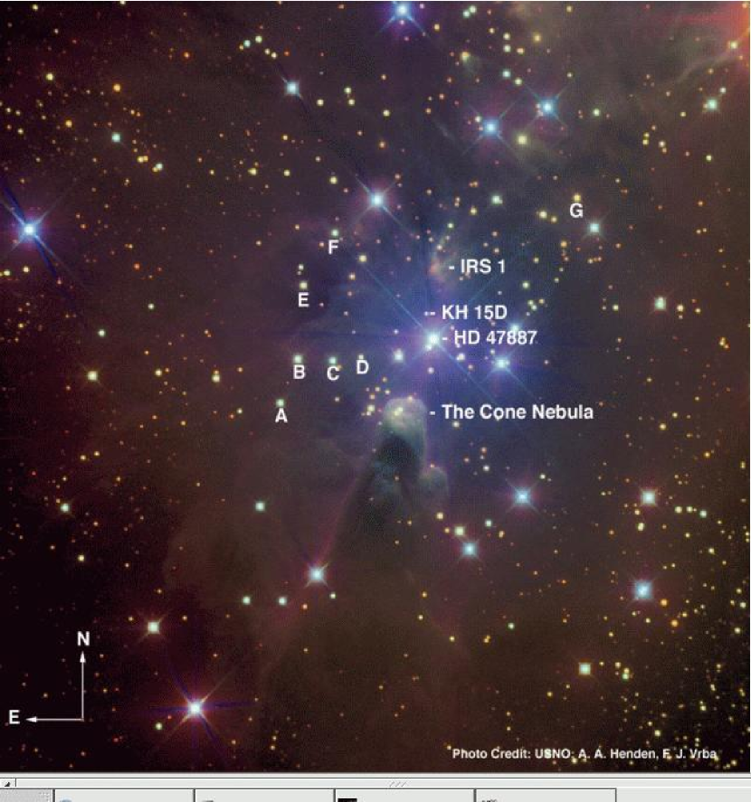
Figure 1: KH 15D and the surrounding region of NGC 2264. Local comparison stars used in the photometry of KH 15D are labeled A–G. North is up and east is to the left.

KH 15D, an extraordinary pre-main-sequence eclipsing binary system, is located in the young (2–4 Myr) open cluster NGC 2264 ($d$ $\approx$ 760 pc). In 1970, a Russian circular announced the discovery of eight new variable stars in NGC 2264 (Badalian & Erastova 1970). KH 15D was among these, and was given the name SVS 1723. It was found to vary by 1.1 mag and was classified as an irregular variable. In 1972, the new variables discovered by Badalian & Erastova (1970) were included in the 58th Name-List of Variable Stars (Kukarkin et al. 1972), and KH 15D was given the name V582 Mon. Prior to October 2000, KH 15D had been observed in various surveys of the open cluster NGC 2264. Flaccomio et al. (1999) and Park et al. (2000) both observed KH 15D at least once while the system was bright and included it in their catalogs, each identifying it as #391 and #150, respectively. Earlier surveys of NGC 2264 (Herbig 1954; Walker 1956; Vasilevskis, Sanders, & Balz 1965) did not identify KH 15D as a cluster member most likely because of its proximity to the B2 III star, HD 47887 (see Fig. 1). Its light was simply lost in the bright glow of the B2 III star.

This object gained its notoriety as KH 15D when it was reported to have unusual properties in 1995 based on a project at the Van Vleck Observatory (VVO) to photometrically monitor star-forming regions (Kearns & Herbst 1998). This object was observed to undergo eclipses that were remarkably deep ($\sim$3.5 mag in $I$) and unusually long ($\sim$16 days in 1999/2000). Of central interest was the evolution of the shape and duration of the eclipses that had been observed over a 5-year period (Hamilton et al. 2001). Out of eclipse, the observable star in this system was determined to have a spectral type of K6/K7 (Hamilton et al. 2001; Agol et al. 2004), while during eclipse, the observed spectrum was simply an attenuated version of that out of eclipse.

An international campaign to monitor this intriguing system was begun during July 2001. The primary goal of this project was to obtain much information about the structure of the intervening material. Continued photometric observations from around the world provided nearly complete coverage of three consecutive eclipses during the 2001/2002 observing season (Herbst et al. 2002). These consecutive eclipses demonstrated that, in addition to the yearly changes observed in the phased data, differences in the shape of each individual eclipse could be observed over the course of a season. The shapes of ingress and egress were successfully modeled by the steady advance or retreat of a “knife edge” across a limb-darkened star. In order to match the duration of ingress and egress, however, Herbst et al. (2002) determined that the occulting edge must be inclined by $\sim$15$\arcdeg$ to the motion of the star. These authors also reported that the object’s color becomes slightly bluer during eclipse, which indicates that most (if not all) of the light received during eclipse is due to scattering.

Polarization measurements made by Agol et al. (2004) and Gary Schmidt (private communication) show that out of eclipse, the system exhibits low polarization consistent with zero. During eclipse, however, the polarization is observed to increase to roughly 2% across the optical spectrum. These results support the conclusion that the star is likely completely eclipsed so that the flux during eclipse is due entirely to scattered radiation, and that the obscuring material is most likely made up of relatively large grains ($\sim$10 $\mu$m; Agol et al. 2004).

High-resolution spectra obtained during the December 2001 eclipse (Hamilton et al. 2003) revealed that the system is still undergoing accretion and driving a bipolar outflow. Recently, extended molecular hydrogen emission near 2 $\mu$m was observed spectroscopically by Deming, Charbonneau, & Harrington (2004). Given the spatial extent of the emission, and the observed H₂ line profile, Deming et al. (2004) suggest that the ambient H₂ gas is being shocked by a bipolar outflow from the star and/or disk. Further evidence for an extended and well-collimated outflow was provided by Tokunaga et al. (2004), who obtained broad-band and narrow-band infrared images of KH 15D, showing a jet-like H₂ emission filament that extends out to $\sim 15\arcsec$ from the object. The position angle ($\sim$20°) of the in-eclipse polarization is nearly parallel to this H₂ filament (Agol et al. 2004).

Many hypotheses have been proposed since 2001 to explain the evolving eclipses of KH 15D. Most of these involve circumstellar material in some way. Hamilton et al. (2001), Herbst et al. (2002), Winn et al. (2003), and Agol et al. (2004) all proposed the idea of an edge-on circumstellar disk with a warp that periodically passes in front of the star. Barge & Viton (2003) proposed that the eclipses were caused by an orbiting vortex of solid particles, and Grinin & Tambotseva (2002) suggested that an asymmetric common envelope in a binary system could accurately reproduce the eclipses. Historical studies by Winn et al. (2003) found that observations made between 1913 and 1950 were consistent with no eclipses. Johnson & Winn (2004, hereafter JW04) discovered that between 1967 and 1982, the system alternated between bright and faint states with the same period as observed today, but 180$\arcdeg$ out of phase with the current eclipses. Additionally, the eclipse depth was much smaller (only 0.67 $\pm$ 0.07 mag in $I$ instead of 3.5 mag), and when out of eclipse, the system was brighter by 0.9 $\pm$ 0.15 mag than it is today (JW04). While Herbst et al. (2002) first suggested the possibility of a binary companion, the light curve between 1967 and 1982 led JW04 to believe that the light from a second brighter star once contributed to the flux coming from this system, and that the second star is now completely obscured. These results have been confirmed and extended by data obtained at various observatories between 1954 and 1997 (Johnson et al. 2005).

Models of the KH 15D system that explained the historical and modern-day light curves were put forward almost simultaneously by Winn et al. (2004) and Chiang & Murray-Clay (2004). Each model involves an eccentric pre-main-sequence binary whose motion periodically carries it behind a precessing circumbinary disk. These models are supported by the results of a recent high-resolution spectroscopic monitoring program of KH 15D: Johnson et al. (2004) have observed radial-velocity variations that are consistent with a binary companion with an orbital period in agreement with the 48-day photometric period.

In summary, KH 15D is now known to be a pre-main-sequence binary system with a strongly eccentric orbit of 48.38 days. The brighter component B is currently totally obscured by the circumbinary ring or disk, while only the fainter member A emerges from behind the obscuring material for just less than half the period. To explain the secular variations observed in the light curve over the past 9 years, it has been suggested that the eclipses occur whenever the motion of a star carries it behind the ring, with a period equal to that of the binary orbital period. If this ring is also precessing, it would be possible to explain the changing length of the eclipse.

In this paper we present the analysis of photometric data on KH 15D obtained at VVO between 1995 and 2000, color data obtained at the Cerro Tololo Inter-American Observatory (CTIO) during the 2001/2002 season, and the results of the 2002–2004 observing campaigns as compared to those of 2001/2002. Section 2 describes the principal sources of optical photometric observations, the data reduction, and the resulting photometry for each participating observatory in the 2002–2004 campaigns. A comparison of individual data sets is shown in Section 3, while the results and analysis of these data are presented in Section 4. A brief discussion of our findings in light of the recent models is also presented, while a more complete interpretation is deferred to a future paper (Winn et al. 2005, in preparation).

2 Observing Procedure, Reductions, and Photometry

The principal sources of optical photometric data analyzed here are telescopes of 0.6–2.2 m aperture. These include the US Naval Observatory’s (USNO) Flagstaff Observing Station in Arizona, Mount Maidanak Observatory (MMO) in Uzbekistan, VVO in Connecticut, the European Southern Observatory (ESO) and CTIO in Chile, Kitt Peak National Observatory (KPNO) in Arizona, Wise Observatory in Israel, Teide Observatory in the Canary Islands, and Konkoly Observatory in Hungary. We also obtained data with automated telescopes at the Tenagra Observatory in Nogales, Arizona, and the Katzman Automatic Imaging Telescope (KAIT), located at Lick Observatory atop Mt. Hamilton in California.

While attempts were made to encourage uniformity in observing and reduction procedures within the initial group of participating observatories during the 2001/2002 season, the excitement that this object ignited inspired observers at telescopes around the world to contribute data to this project during the subsequent seasons. Variations in seeing, image quality, sky brightness, flat-fielding procedures, and CCD characteristics made it impossible to enforce substantial uniformity. Although the photometry parameters varied widely between data sets for the 2002–2004 observing seasons, which are discussed in detail here, we compared data obtained at different observatories on the same nights to search for consistency, as described below. It should also be noted that not all observatories used the same reference stars in their data reduction.

We begin by listing the contributing observatories, telescopes, CCD parameters, filters, and dates in Table 1. (UT dates are used throughout this paper.) Most observations were made with a Cousins $I$ filter to reduce the nebular contamination of NGC 2264, as well as the contribution from the nearby B2 III star, HD 47887, which is $39\arcsec$ away. Here we will discuss the 2002–2004 data in detail. Exposure times varied per observatory according to telescope and CCD pixel size. Observatories with similar observing procedures and reduction/photometry techniques are grouped together. Photometry parameters for each dataset from 2002–2004 are included in Table 2.

2.1 USNO, Flagstaff Station

2.1.1 Observing Procedure and Reduction

Attempts were made to observe KH 15D nearly every clear night during the 2002/2003 observing season at the USNO, Flagstaff Station. $B$, $V$, $R$, and $I$ filters were used while KH 15D was bright, and only $V$, $R$, and $I$ during eclipse. In 2003/2004, multiple observations were obtained during three consecutive egresses using only the $V$, $R$, and $I$ filters. Exposure times generally ranged from 2 to 3 minutes, depending on whether the object was bright or faint. All frames were bias-subtracted and flat-fielded in real time by local code.

2.1.2 Photometry

Photometry was performed on individual frames with an aperture radius that depended on the full width at half-maximum (FWHM) of unblended stars in the image. To maximize the signal-to-noise ratio (S/N), a radius of $\sim 1.5\times{\rm FWHM}$ was employed. The background parameters were set such that the scattered light from HD 47887 was minimized (see Table 2).

Differential photometry of KH 15D was performed using seven reference stars selected from all-sky photometry obtained with the 1.0 m telescope at the USNO, Flagstaff Station. A finding chart for the 7 comparison stars is shown in Figure 1, and the adopted standard Johnson $UBV$ and Kron-Cousins $RI$ magnitudes for each comparison star is given in Table 3. To determine the magnitude for each frame ($B$, $V$, $R$, and $I$), the $m_{true}-m_{instrumental}$ magnitude difference was calculated for each non-saturated standard star. This difference was then applied to the $m_{instrumental}$ magnitude of KH 15D. No color terms were used since the USNO filters are well matched to the standard system and the local standards span the colors of KH 15D. The resultant uncertainty includes the spread in the $\Delta m$ due to not including a color term.

2.2 Van Vleck Observatory (VVO), Tenagra Observatory, and KAIT

2.2.1 Observing Procedure and Reduction

KH 15D was generally observed once every clear night at VVO, Tenagra, and KAIT. Typically, five 1-minute exposures were obtained per night; however, during ingress and egress, VVO increased the number of exposures. All images obtained at VVO and Tenagra were bias-subtracted, corrected for dark current, and flat-fielded using standard IRAF tasks (CCDPROC). Images obtained at KAIT were bias-subtracted, corrected for dark current, and flat-fielded automatically using a local code (Li et al. 2003). After each image was processed, sets of five were averaged to increase the S/N, and the result was aligned to a single reference image using an IDL (Interactive Data Language) code. The FWHM for stars in each image was measured using the IRAF task IMEXAMINE, and was used to assess the seeing on that night. Any image that exhibited a very large FWHM ($\sim$ 4.5$\arcsec$ or larger) was not used.

2.2.2 Photometry

For the analysis performed here, the average FWHM for the observing season was calculated and used to determine the size of the aperture radius utilized in the photometry process. This method was chosen so that all the data from one season could be processed and analyzed most simply in batch mode. We find that the standard deviation from this mean is typically less than 0.5 pix. To maximize the S/N, a radius of $\sim 1.5~{}\times<{\rm FWHM}>$ was chosen.

Instrumental magnitudes and uncertainties were computed for all the local comparison stars (see Fig. 1) and KH 15D using the IRAF task PHOT. Calibration of the instrumental magnitudes from one observation to the next was accomplished by means of a set of comparison stars, which were averaged together to produce a synthetic stable comparison. However, since even these stars are variable at some level, the final set of stars used were identified by an iterative process, and represent the most stable ones, with a typical standard deviation of 0.005 mag based on their night-to-night scatter. Stars A, C, E, and G (see Fig. 1) were found to be most stable and were used as the comparison stars for both the 2002/2003 and 2003/2004 seasons at VVO. Due to saturation issues, stars A, C, E, and F were used for the Tenagra images, while only stars C, E, and F could be used for the KAIT data due to the small size of the detector. A time series of differential magnitudes relative to the synthetic comparison star was then produced. To place KH 15D on the standard magnitude scale, the adopted $I$-band magnitudes (converted to flux) of each comparison star were averaged to produce an $<I>$ comparison magnitude. This was then added to the differential magnitudes calculated for KH 15D during the 2002/2003 and 2003/2004 observing seasons.

2.3 Mount Maidanak Observatory (MMO)

2.3.1 Observing Procedure and Reduction

KH 15D was observed multiple times on nearly every clear night at MMO (Uzbekistan) during the 2002–2004 observing seasons. Exposure times typically ranged from 2 to 5 minutes, and all observations were made with a Bessell $I$ filter. Raw frames were bias-subtracted and flat-fielded using the IMRED package within the IRAF environment. Sky flat-field images were usually taken for each night, but in some cases only dome flats were available.

2.3.2 Photometry

Differential magnitudes for KH 15D were computed in reference to star 16D from Kearns et al. (1997). In order to place these differential magnitudes onto our standard scale, we needed to know the true magnitude of 16D. Thus, 16D was photometered during the 2001–2004 seasons at VVO in addition to the 7 local standards and KH 15D (see Section 2.2.2), and the weighted average flux of 16D for the season was converted to a magnitude. This magnitude was then added to the differential magnitudes computed for 15D at MMO. The weighted average $I$ magnitudes computed for 16D between 2001 and 2004 are given in Table 4. Since error bars were not produced when computing the differential magnitudes, we could not assign formal photometric uncertainties to these data.

2.4 Konkoly Observatory

2.4.1 Observing Procedure and Reduction

KH 15D was observed multiple times on nearly every clear night at Konkoly Observatory during the 2002/2003 observing seasons. Exposure times ranged from 2 to 20 minutes, but were typically 5 minutes. All observations were made with a Cousins $I$ filter. Raw frames were bias-subtracted and flat-fielded using the IMRED package within the IRAF environment. Sky flat-field images were usually taken for each night, but in some cases only dome flats were available.

2.4.2 Photometry

The differential magnitudes of KH 15D were measured in reference to local secondary standard stars C, D, and F (see Fig. 1). To determine the raw magnitudes of stars in the frames, aperture photometry was performed using the IRAF/DAOPHOT package (Stetson 1990). The FWHM of the stellar profile was determined for each night and an aperture of $\sim 1.5\times{\rm FWHM}$ was chosen. The ring from which we estimated the background contribution to the measured fluxes started 2 pixels from our aperture and had a width of 5 pixels in every case.

The differential magnitudes were calculated by defining the variable’s brightness as $\Delta I=I_{var}-I_{comp}$. These differential magnitudes ($\Delta I$) were transformed onto the standard photometric system by taking the adopted $I$ magnitudes (converted to flux) of each comparison star and averaging them together to produce an $<I>$ comparison magnitude. This was then added to $\Delta I$ to get the true $I$ magnitude of KH 15D. No color term was applied since the Konkoly $I$-band filter is well matched to the standard system. Finally, three Cousins $I$ magnitudes of KH 15D were calculated on each frame by adding the magnitudes of the comparison stars to the differential magnitudes. We calculated the brightness by averaging the three different fluxes determined for KH 15D. The uncertainty of the brightness of KH 15D was estimated from the standard deviation of the three individual magnitudes.

2.5 Teide Observatory

2.5.1 Observing Procedure and Reduction

KH 15D was observed multiple times every clear night during the 2002/2003 observing season at the Teide Observatory. Exposure times varied from 5 to 20 minutes, and all observations were made with a Cousins $I$ filter. Raw frames were bias-subtracted and flat-fielded using the IMRED package within the IRAF environment. Sky flat-field images were usually taken for each night, but in some cases only dome flats were available.

2.5.2 Photometry

Differential photometry of KH 15D was performed using an aperture of $0.5\times{\rm FWHM}$. The sky background was computed using a circular annulus with an inner radius of $4\times{\rm FWHM}$ and a width of 8 pixels. Differential photometry and calibration from instrumental magnitudes to real ones was accomplished with respect to the reference stars 16D, 17D, 27D, 31D, and 39D from Kearns et al. (1997).

2.6 Van Vleck Observatory Data from 1995 to 2000

Data obtained at VVO between the years of 1995 and 2000 were re-examined with parameters that were consistent with those of the 2001–2004 observing seasons. This was done so that an absolute comparison between the earliest data and the most recent data could be made. One difficulty in completing this task was the fact that from the fall of 1995 through the spring of 1998, VVO used a chip that was only 512 $\times$ 512 pixels in size. Therefore, only one of the current “standard” stars (D) was available, and it also happened to be the most variable star. Therefore, we consulted the original photometric studies of NGC 2264 conducted at VVO (Kearns et al. 1997; Kearns & Herbst 1998) and examined 5 of their quoted comparison stars (16D, 17D, 21D, 27D, and 31D). Since these stars did not have known magnitudes, each was photometered on the images taken at VVO during the 2001–2004 observing seasons, allowing us to determine their magnitude on our standard scale. Table 4 lists the weighted average $I$ magnitude and uncertainties for each star during 2001–2004. Once a standard magnitude was known for each comparison star, all 5 stars and KH 15D were photometered on the images obtained at VVO between 1995 and 1998. Table 5 lists the comparison stars used for each season.

2.7 European Southern Observatory (ESO)

2.7.1 Observing Procedure and Reduction

The ESO observations of KH 15D contributed here were the byproduct of a larger photometric monitoring program of NGC 2264 (Lamm et al. 2004). Full details describing the observing procedure, reduction methods, and photometry parameters can be found in Lamm et al. (2004). In summary, monitoring of NGC 2264, and hence of KH 15D, took place during a period of two months between 30 December 2000 and 01 March 2001 with the Wide Field Imager (WFI) on the MPG/ESO 2.2 m telescope on La Silla (Chile). All observations were carried out with a Cousins $I$-band filter. The WFI consists of a mosaic of 4 $\times$ 2 CCDs with a total array size of 8K $\times$ 8K. Exposures of 5 s, 50 s, and 500 s were obtained, but the data used in this contribution come only from the 500 s images. Image processing was done separately for each of the individual WFI chips using standard IRAF tasks. Each image was bias-subtracted using the overscan region in each frame, and flattened using an illumination-corrected dome flat.

The data presented here are based on differential photometry relative to a set of non-variable reference stars. The DAOPHOT/APPHOT task was used to measure the brightness of KH 15D. The aperture was chosen to be 8 pixels (1.9$\arcsec$) in diameter for all measurements in order to maximize the S/N. The sky was calculated as the median of an annulus with an inner diameter of 30 pixels (7.1$\arcsec$) and a width of 8 pixels centered on KH 15D. Because only differential magnitudes were calculated for the ESO data, we computed the average out-of-eclipse magnitude for the 2000/2001 season based only on the data obtained at VVO. An appropriate out-of-eclipse magnitude was then added to the ESO differential magnitudes such that these data could be placed on our standard scale.

2.8 Cerro Tololo Inter-American Observatory (CTIO)

2.8.1 Observing Procedure and Reduction

KH 15D was observed extensively during the 2001/2002 observing season with the CTIO/Yale 1 m telescope. All observations were made with a single instrument (ANDICAM; see DePoy et al. 2003 for a description) using Johnson $V$ and $I$ filters. KH 15D was observed on nearly every usable night between 30 August 2001 and 18 April 2002. Typically, several images were obtained each night using 300 s exposures. The data were reduced in the usual manner using standard IRAF routines: an overscan (bias) was subtracted and a flat-field was applied to all the images.

2.8.2 Photometry

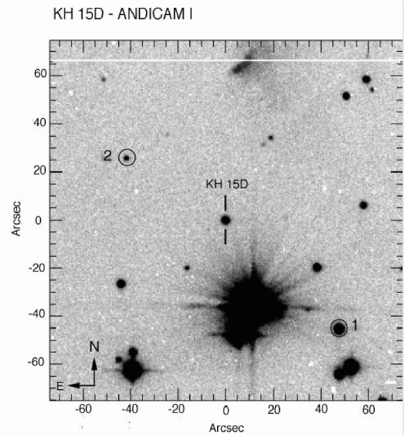
Figure 2: KH 15D and the local comparison stars used for the CTIO photometry. North is up and east is to the left.

KH 15D was measured relative to two nearby stars shown in Figure 2. Labeled as “1” and “2,” they are also known as 5D and 25D from Kearns et al. (1997), with $I$ = 13.250 $\pm$ 0.001 mag and $I$ = 16.464 $\pm$ 0.005 mag, respectively. We find that neither comparison star varied by more than 0.005 mag over the duration of the observations of KH 15D. A 3.6$\arcsec$ diameter aperture was synthesized on each of the CCD images for both of the reference stars and KH 15D using standard IRAF aperture photometry routines. The sky was determined in a 4$\arcsec$ to 6$\arcsec$ annulus immediately adjacent to each of the sources.

We calibrated the measurements of KH 15D relative to the two stars using images obtained at the 1.3-m McGraw-Hill telescope of the Michigan-Dartmouth-MIT (MDM) Observatory. The data were obtained on the photometric night of 19 October 2003. The scale for the 1024 $\times$ 1024 pixel CCD that we used is 0.5$\arcsec$ pixel^-1. Throughout the night we observed photometric standard stars taken from Landolt (1992) at a range of airmasses. Near the end of this night we also obtained 12 $V$-band and 7 $I$-band images of the KH 15D field.

We reduced the data using standard IRAF techniques, including bias-subtraction and flat-fielding using twilight-sky flats obtained during the evening twilight of the same night. We performed aperture photometry on the McGraw-Hill data, using a 20 pixel (10$\arcsec$) diameter aperture for both the standard stars and the target stars in the KH 15D field. The seeing throughout the night was roughly 1.4$\arcsec$, so aperture effects should be small. A photometric solution was found using all 36 standard-star measurements in $V$ and $I$. We solved only for the zero point and extinction coefficient terms and held the color term constant at zero. This solution was then applied to the KH 15D field stars, and the calibration was used to convert the relative photometry to the standard system. We estimate that ignoring the color term in our calibration observations and between the MDM and the CTIO/Yale observations gives a systematic error in the KH 15D light curve of $\leq$0.02 mag. This is based on intercomparison of other standard-star measurements.

3 Comparison of Photometric Data

This paper combines a number of data sets obtained at various observatories, analyzed by different means, as described in the preceding sections. Before beginning the process of analyzing the results of these data, random and systematic errors between data sets were assessed. To accomplish this, we selected all the photometry obtained at different places on the same Julian Date. If there were multiple observations made at a given observatory, a nightly mean was calculated. This nightly mean was then used in the analysis described below. Out-of-eclipse and in-eclipse observations were analyzed separately since the photometric errors are typically much larger during eclipse owing to the faintness of the object. Additionally, times of ingress and egress were avoided since the magnitude of the system changes too rapidly for comparison of data, even as close as one day apart. Each season is addressed separately.

3.1 The 2001/2002 Observing Season – The CTIO Contribution

One of the main objectives of the observing campaign of 2001/2002 was to study, in detail, the eclipse of December 2001. The original contributing observatories included Wise, VVO, MMO, USNO, and KPNO, and the results were reported by Herbst et al. (2002). We now have data from the CTIO/Yale 1 m telescope that has provided us with perhaps the highest sampling rate yet of the eclipses that occurred during the 2001/2002 season. These are shown in Figure 3. The central reversal is evident in these data, as well as some variation in the shape of ingress/egress from eclipse to eclipse. Additionally, substantial variability is seen outside of eclipse, as explored further in Section 4.1.2.

Since these data were originally obtained through Johnson $V$ and $I$ filters, we could not immediately combine them with the rest of our Cousins $I$-band data. The coverage of nearly 5 eclipses, including dense sampling throughout ingress and egress, provided excellent color information about this system. We therefore examined the Johnson colors separately from the other data sets and present the results in Section 4. However, in order to add these Johnson data to the full $I$-band light curve, we computed a transformation from Johnson $I$ to Cousins $I$ by comparing nearly simultaneous Johnson $V$-band and Cousins $I$-band data that were obtained at the USNO (see next section).

3.2 The 2002/2003 Observing Season

In 2002/2003, seven different observatories contributed to the light curve of KH 15D (see Table 1). To evaluate the systematic differences between each contribution, we began by selecting all the data that were obtained on the same Julian Dates outside of eclipse, for the entire observing season. We define “out-of-eclipse” to correspond to phases between 0.3 and 0.7 for both the 2002/2003 and 2003/2004 seasons. The out-of-eclipse 2002/2003 data are shown in Figure 4. For each Julian Date, the mean brightness of the star was formed based on all measurements. These contributions might include a single observation from one observatory and a mean observation (due to multiple exposures throughout the night) from another. The difference between each observatory’s measurement and the total nightly mean was then calculated and examined as a function of the total mean brightness. A histogram indicating the number of times an observatory’s measurement differed from the mean by 0.01 mag, 0.02 mag, etc. is shown in Figure 5. In general, there appears to be good agreement between the data sets. Most observations differ from the mean by $\sim$0.01 mag, which is typically the size of the estimated random errors associated with the photometry. Thus, we can say that the data sets are consistent with each other to within $\sim$0.02 mag. Variations in the light curve on the order of $\sim$0.08 mag are observed out-of-eclipse (see Fig. 4), which we take to be real, and not an artifact of combining the data sets. This will be explored further in Section 4.

Figure 6 shows multiple data obtained on the same Julian Dates while in deep eclipse during 2002/2003. We defined “deep eclipse” to correspond to phases between 0.83 and 0.17 for both 2002/2003 and 2003/2004, with phase = 0.0 (and 1.0) representing the approximate phase for mid-eclipse. The same analysis described above was performed on these data. Figure 7 shows that the differences of each observatory’s observation from the mean is on average $\sim$0.15 mag, which is consistent with the photometric observational errors.

3.3 The 2003/2004 Observing Season

In 2003/2004, only four observatories contributed to the light curve of KH 15D (see Table 1). There were significantly fewer multiple observations out-of-eclipse during 2003/2004 as compared to 2002/2003. We compared these individual measurements in the same manner as discussed above. The agreement between these data sets is not as good as was seen in the previous season. On average, the data from Tenagra were $\sim$0.04 mag brighter than those from VVO, and the data obtained at VVO were $\sim$0.02 mag brighter than those obtained at MMO (although that is not always the case). There are generally only 2 observations contributing to the calculation of the mean on any given night. Therefore, the difference between each observatory’s measurement and the mean gives us a sense of the systematic differences between each data set. The average difference is $\sim$0.02 mag, which is slightly larger than the typical photometric errors ($\sim$0.01 mag or smaller). The in-eclipse data from 2003/2004 showed a great deal of scatter, but for the most part, appear to be correlated with each other. On average, the data depart from the calculated mean by $\sim$0.15 mag, which is on the order of the quoted photometric errors associated with the in-eclipse measurements.

Overall, the data sets from both 2002/2003 and 2003/2004 mesh fairly well, and do not appear to be grossly different from each other. Therefore, we feel confident that the shape of the light curve and the depth of the eclipses are accurate to within $\sim$0.02 mag out-of-eclipse and $\sim$0.15 mag in deep eclipse.

4 Results and Analysis

The full data set now contains 6694 measurements of Cousins $I$ magnitude covering nine seasons of observation between 1995 October and 2004 March, as well as additional color measurements. Magnitudes in $I$ are given in Table 6 and colors are given in Table 7. Both tables, in full, are available electronically. In this section we describe the light and color variations and propose a rotation period for the star. We also provide some qualitative guidance to the interpretation of the variations based on the models of Winn et al. (2004) and Chiang & Murray-Clay (2004). Detailed modeling of the photometric (and spectroscopic) data will be done by Winn et al. (2005). We turn first to a discussion of the light variations in $I$, where most of the data are available.

4.1 Light Variations

Figure 8 shows the data from the last two seasons, which is the primary addition to the data set in this paper. Clearly, we have obtained good coverage of a total of nine eclipses over two seasons. Results indicate that the trends noticed by Hamilton et al. (2001) (reduction in amplitude of the central reversal and widening of the eclipse) are continuing, and it would appear that the duration of the eclipse is now about one-half of the period (compare with Fig. 3). The shapes of ingress and egress are not identical and show some level of variation, not only from eclipse to eclipse, but also from year to year. Since 2001, the duration of the eclipse has been growing by roughly 2 days year^-1. However, as will be seen in Section 4.1.2, this has not always been the case. In earlier years, such as from 1998/1999 to 1999/2000, the change in eclipse length was close to 1 day.

In Figure 9, the last two seasons are compared with the seven previous ones for which modern, CCD photometry is available. Some of the features and a distinct secular variation of the light curve can be seen. Here, it appears that the out-of-eclipse brightness of the star has not changed by more than $\sim$0.1 mag since 1995, while the depth of the eclipse has grown by $\sim$1 mag over that same interval. In fact, it appears as though the eclipse depth has been increasing at a rate of $\sim$0.2 mag year^-1.

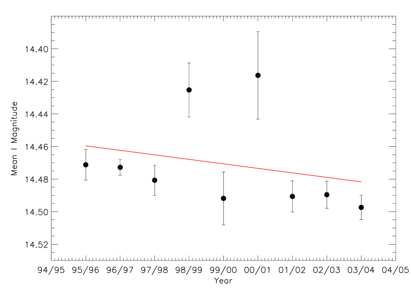
Figure 10: The mean out-of-eclipse $I$ magnitude as measured at VVO from 1995 to 2004. The error bars represent the standard deviation of the mean for each year. The straight line is simple linear fit to the data. It appears as if the star might be fading a bit with time, but it is unclear whether this is a significant trend.

To determine the best estimate of the mean $I$ magnitude out-of-eclipse, we looked solely at the data obtained at VVO since it was the only observatory from which we had data for every year. We began by calculating a mean $I$ magnitude per year to see if there was any variation in the out-of-eclipse brightness with time. The phases that corresponded to the out-of-eclipse state changed as the width of the eclipse evolved with time (discussed below), and are listed in Table 8. Figure 10 shows the mean $I$ magnitudes versus observing season at VVO. The straight line represents a simple linear fit to the data. It appears as if the currently visible star might also be fading a bit, but we cannot be sure whether this is a significant trend. As shown below, the increasing depth of the eclipse is accompanied by an increased time duration and a diminishing height for the central brightness reversal. The current data show that these trends, noticed previously (see Hamilton et al. 2001; Herbst et al. 2002), have continued in the last two seasons.

4.1.1 Brightness of the Currently Invisible Star

During the first season of monitoring at VVO there was one unusually bright data point, taken on only the sixth night that the system was observed. Repeated checks have shown that this is a valid datum and cannot be discarded as an error. As will be shown below, its phase also corresponds to a point close to mid-eclipse. We now interpret that point as the only observation in our data set during which the relatively unobscured light from the currently invisible star (B) was seen directly. This point occurred close to periastron when star B was peaking above the disk for just about the last time. On that night, the system’s light was only due to star B, since star A was hidden behind the disk. If this interpretation is correct, it means that the magnitude of star B is equal to or brighter than $I$ = 14.01 $\pm$ 0.01 (see Table 6). Since star B might also have been partly hidden itself, we cannot say for sure based on one measurement whether star B is brighter than $I$ = 14.01 $\pm$ 0.01, but it certainly cannot be fainter.

This conclusion is consistent with the historical light curve. Johnson et al. (2005) show that prior to 1990, the system was at times as much as 1 mag brighter than it appears today. If we take the difference between the combined light (star A + star B) and the light of star A alone to be $-1.0$ mag, then the magnitude difference between star A and B is 0.45. The mean $I$ magnitude out-of-eclipse based on the VVO data (see Fig. 10) shows that star A has a mean $I$ = 14.47 $\pm$ 0.03 mag. Assuming a minimum $I$ magnitude of 14.01 $\pm$ 0.01 for star B, the mean brightness of star B is 0.46 $\pm$ 0.03 mag brighter than star A. To make further progress we wish to phase the light curve with the appropriate period for the system, a task to which we now turn.

4.1.2 The 48-day Period

It is important to establish the period of this system to the highest accuracy possible so that the data can be properly phased and the evolution of the light curve with time correctly displayed. It is now known that the 48-day period comes from the orbital motion within the binary. As such, the most definitive determination of the period should come from radial-velocity measurements and the spectroscopic-binary solution. This yields a period of 48.38 days with an uncertainty of about 0.01 days (Johnson et al. 2004). The problem with this method is that only a portion of the full orbit of one star can currently be seen, and it is the part near apastron which provides the least leverage on the solution. A second complication is that the visible star may suffer from a Rossiter effect (Worek 1996) of unknown size as it enters or emerges from eclipse, depending on the inclination angle of the rotation axis to the line of sight. Therefore, the data that provide the greatest leverage on the radial-velocity solution (i.e., those taken during late egress or early ingress) may also be the data which are compromised in this regard.

Hence, we believe it is important to ask independently of the radial velocities whether the period of the system can be determined. The problem with the photometric method is, of course, that the light curve is evolving with time due to the progressive occultation by a foreground screen. This puts an additional time-dependent behavior into the system, albeit on a much longer time scale than the orbital period.

To proceed, we first did a Fourier transform of all of the modern photometric data using the Scargle Periodogram technique (Scargle 1982; Horne & Baliunas 1986). This yielded a highly significant peak in the periodogram at 48.367 days (see Fig. 11), which we round to 48.37, as discussed below. This is gratifyingly close to the spectroscopic period and to the previously reported photometric period of 48.36 days (Herbst et al. 2002).

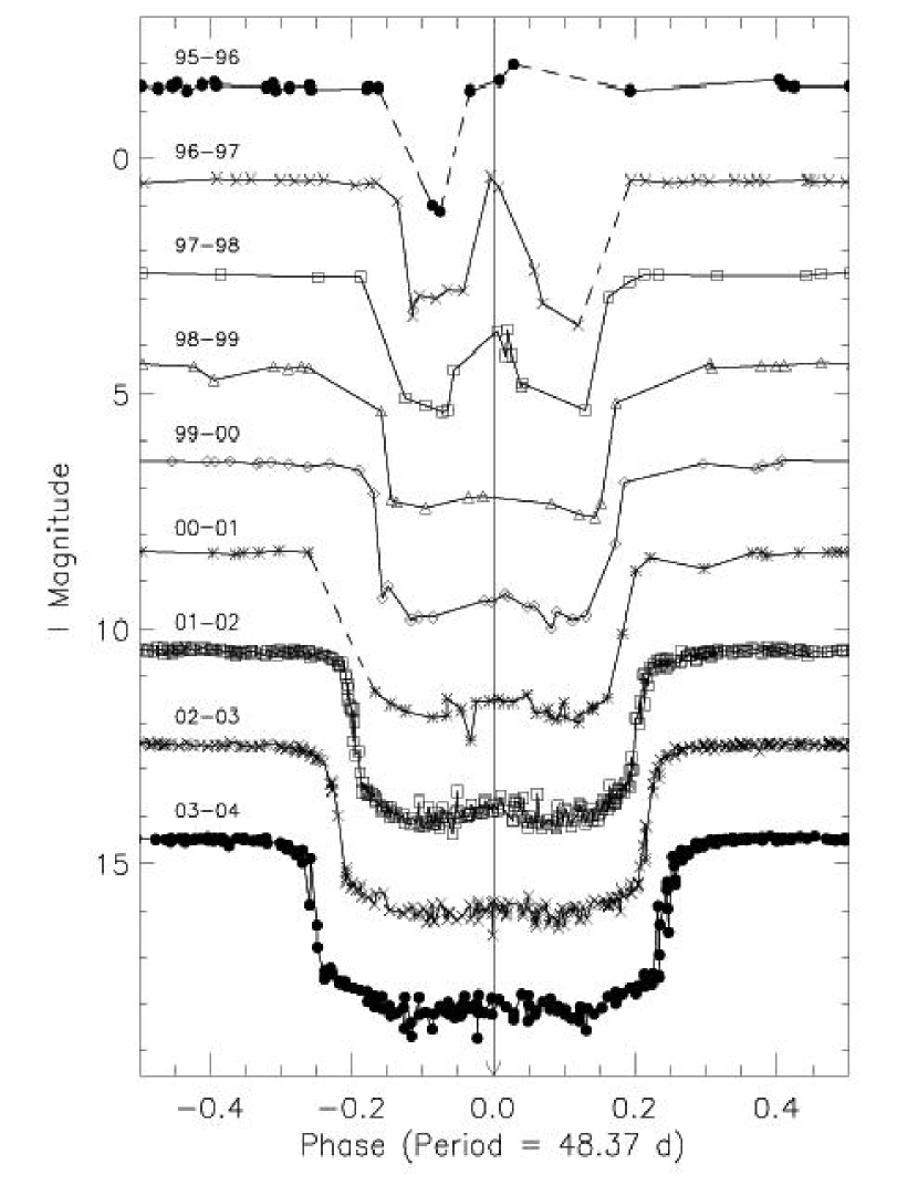
Figure 12: The data from Fig. 9 are shown here, phased with the 48.37 day period. The evolution of the light curve phased at this period may tell us something about the dynamical processes that are occurring.

We attempted to refine the photometric period by focusing on a particular feature in the light curve whose phase we believe is stable and whose location we could determine from season to season. The only such feature that exists is the peak of the central reversal (see Fig. 12), which we take to be the point in the orbit when the currently unseen star is closest to the edge of the obscuring cloud. Assuming that this is a stable, fixed location in the orbit, if we could phase these central peaks we would have a good estimate of the period. Unfortunately, it turns out that this method lacks discrimination because the location of the central peak is not sufficiently well defined by the light curves, especially the early ones where the data density is too low. A difference of 0.01 days in period is not significant and does not affect our results, as it corresponds to only 0.75 days over the 75 cycles covered by our monitoring and the early data do not constrain the time of the central peak to better than that.

Therefore, we find it impossible to improve on the accuracy of the period determinations with just these data. It might be possible to do this photometrically using the historical data, but any discussion of that is postponed to a later contribution (Winn et al. 2005, in prep.). Here we simply adopt the result of the periodogram analysis, 48.37 days, noting that it is consistent with the spectroscopic determination; the 0.01 day difference does not affect any of the analysis or conclusions reported here.

4.1.3 An Additional Periodicity – The Rotation Period of the Visible Component

During the 2001–2004 observing seasons, a great deal of effort was made to observe KH 15D out-of-eclipse as well as in eclipse. Significantly more data populated the bright phase of the light curve during these seasons than ever before, and small-scale variations ($\sim$0.08 mag over the course of 8–14 days in 2002/2003) are evident (see Fig. 4 and Section 3.1). Since the visible star in the KH 15D system is a weak-lined T Tauri star (WTTS; Hamilton et al. 2001), it is most likely spotted in some fashion. It has been determined that this K7 star is still actively accreting (Hamilton et al. 2003), and could therefore exhibit accretion hot spots on its surface, in addition to any dark, magnetically induced star spots. If this is the case, a closer look at the out-of-eclipse data from the 2001–2004 seasons may provide an estimate for the rotation period of the star.

The analysis above indicates that systematic errors between data sets are relatively small, being at the level of 0.02 mag or less. However, when searching for the tiny amplitudes (less than 0.1 mag) that may characterize rotationally induced spotted-star variations, even errors of this size may make the search more difficult. Therefore, we have searched each observatory’s data set independently for periodicity during the out-of-eclipse phases. It is also prudent to confine the search to a single season of observation since spots are well known to evolve on time scales of less than one year. Hence, one rarely finds phase coherence of spot variations extending over more than one observing season.

Detecting spots on WTTSs that are not undergoing eclipses is difficult enough, and generally only 15% or less of the stars in a cluster field will exhibit coherent periodic variations over a season’s observing. In this star we have greater difficulty because during about half the observing season the star is in eclipse. Nonetheless, we have found that periodogram analyses of the available data sets reveals highly significant periods in three cases (see Fig. 13), as listed in Table 9. Notably, two of these periods are identical to within the errors, averaging to 9.6 days. The chance of finding two exactly equal, highly significant periods in these data is vanishingly small if the periodicity is not real; we thus identify the detected period as the likely rotation period of the visible star. It is interesting that the third significant period found in the periodograms (7.95 d) is very close to the beat period between 9.6 and 48.37 days.

Supporting evidence for our interpretation comes from the measured $v\thinspace$sin$(i)$ of the star. As discussed in Appendix A, we derive a value of $v\thinspace$sin$(i)$ = 6.9 $\pm$ 0.3 km s^-1 for the visible component based on high-resolution spectra obtained out of eclipse. Since sin$(i)$ is likely to be very close to 1.0 for this star (assuming that the spin and orbital angular momenta vectors are nearly aligned), one can easily calculate that for a radius of $R=(1.3\pm 0.1)\,$R_⊙ (Hamilton et al. 2001), the expected rotation period is 9.6 $\pm$ 0.1 days, consistent with our result. Both the photometry and spectroscopy of this system out-of-eclipse concur in suggesting a rotation period of 9.6 days for the visible component. To within the errors, this is a 5:1 resonance with the orbital period (48.37/5 = 9.67), although it is not clear whether this is physically significant or just a numerical coincidence.

A rotation period of 9.6 days is somewhat long for a 0.6 M_⊙ WTTS in NGC 2264, although not unprecedented. The (bi)modal values for stars more massive than 0.25 M_⊙ are around 1 and 4 days. However, about 12% of the 182 cluster stars in that mass range with known rotational periods have $P>9.6$ days (Lamm et al. 2005). Could the slightly slower than typical rotation of the visible star in the KH 15D system be caused by a tidal interaction between the components? The effect of tidal friction on rotation can be estimated quantitatively based on the seminal theory of Zahn (1977) for stars with convective envelopes. He shows that the synchronization time for a star’s rotation to become tidally locked to its revolution is approximately given by

$$t_{synch}={q^{-2}({a\over R})^{6}},$$

where $q$ is the mass ratio, $a$ is the semimajor axis, $R$ is the stellar radius, and $t_{synch}$ is given in years. Most of the torque in a highly eccentric system will naturally occur at periastron. With $q\approx 1$ and $a/R=13$, we find a synchronization time of $\sim$5 My. Hence, it is not unreasonable to suggest that tidal friction is responsible for some degree of slowing of this WTTS.

We further note that since the orbit is rather eccentric, one would not expect to reach synchronous rotation, but only pseudosynchronous rotation. The pseudosynchronization timescale describes a near synchronization of revolution and rotation around periastron (Hut 1981). Hut (1981) has shown in elegant fashion that for binaries with eccentricities exceeding $\sim$0.3, as must surely be the case for KH 15D, tidal interaction near periastron is expected to produce an equilibrium angular rotation velocity of about 0.8 times the orbital angular velocity at periastron. One may write, therefore, that the pseudosynchronous rotation period ($P_{ps}$) predicted by this theory is related to the orbital period ($P_{orb}$) by

$$P_{ps}={{P_{orb}\over f}{{{(1-e^{2})}^{3\over 2}}\over{{(1+e)}^{2}}}},$$

where $f$ is near 0.8 for $e>0.3$ and is given precisely by Hut (1981).

The range of particular interest for KH 15D is $0.68<e<0.8$ as discussed by Johnson et al. (2004), because these solutions are consistent with the radial velocities and with the inferred masses of the components based on astrophysical constraints. Over this limited range, and somewhat beyond it, $f$ = 0.81 $\pm$ 0.01. Adopting $P_{ps}=9.6\pm 0.1$ and $P_{orb}$ = 48.37 $\pm$ 0.01 yields a rather precise prediction for $e$ of 0.65 $\pm$ 0.01. This is the required orbital eccentricity if the star is in pseudosynchronous rotation and if the theory of Hut (1981) is correct. Remarkably, this eccentricity is very close to those inferred on the basis of two independent methods. As already noted, the orbital solution based on radial velocities, together with astrophysical constraints on the masses of the components, leads to $0.68<e<0.8$, just barely outside of the present result. Model fits to the light curve and its evolution over more than fifty years, by Winn et al. (2004) and Winn et al. (2005, in prep.), also suggest an eccentricity of between 0.55 and 0.7.

Since the rotation rate of the visible component is notably slower than that of most stars of comparable mass and age, and since it agrees so well with the predicted pseudosynchronous period, we suggest that the star has, indeed, been tidally locked into its current configuration. That, in turn, puts a rather severe limit on the possible eccentricity of the orbit, assuming that the locking has reached equilibrium and that the theory of Hut (1981) is accurate in its prediction of $f$. We note that the strong sensitivity of $P_{ps}$ to $e$ means that there is only a very small range of measured rotation periods which would have given consistent results with the orbital solution and light-curve fitting techniques. For comparison, a normal rotation period of around 1–4 days for this star would have predicted a value of $e$ = 0.8–0.95 for this binary, rather extreme solutions that are inconsistent with the other results.

4.2 The Color Behavior

While most of the monitoring has been in the $I$ band due to the brightness of the star during eclipse, we have also obtained some data at other wavelengths which reveal interesting features of the system. Here we discuss the color results obtained at CTIO in 2001/2002 and at the USNO during several seasons. The discovery reported by Herbst et al. (2002) that the star is generally bluer when fainter is confirmed, but we now have much more detailed and intriguing information on the color variations and their phase dependence.

4.2.1 CTIO Observations

Extensive $V$-band and $I_{J}$-band observations were made during the 2001/2002 season at CTIO with the Yale 1 m telescope (see Sections 2.8 and 3.1 for details) and are shown in Figures 14 and 15. The solid and dashed lines in Figure 14 are provided to indicate the approximate beginning of ingress and ending of egress, respectively. While the Johnson magnitudes can be transformed to Cousins for comparison with other data sets, there is no need to do so in this section, so we plot the results in the Johnson system.

The high density of color data obtained at CTIO during this season reveals an interesting new feature of the behavior of KH 15D: it becomes bluer by a small but significant amount in very steady fashion as it enters eclipse and shows an analogous reddening as it emerges from eclipse. This is quite easily seen in both the time and phased versions of the light curves (Fig. 14 and 15, respectively). It is also confirmed by the less dense but more temporally extended color monitoring done at the USNO as described in the next section.

While the general trend of bluer when fainter had been recognized for this star previously (Herbst et al. 2002) and has been seen in other young stars, such as UXors (e.g., Herbst & Shevchenko 1998), the smooth decrease (increase) in $V-I$ seen during ingress (egress) in Figure 15 is remarkable and unprecedented. Before discussing its interpretation, we complete a description of the color behavior during eclipse.

As both Figures 14 and 15 show, the color change that occurs as the star goes into eclipse does not continue smoothly throughout the eclipse. While the data are noisy due to the low brightness of the star at those phases, it is clear that the star does not maintain a steady color with phase during eclipse. Our impression of Figure 15 is that there are actually three phases when the star has its bluest colors, peaking at about $V-I_{J}$ = 1.2–1.3 mag, or 0.3–0.4 mag bluer than the out-of-eclipse value of $V-I_{J}$ = 1.6 mag. These phases occur around $\pm$0.17 and close to phase 0.

It is interesting that there is also a distinctive feature in the light curve at each of these three phases. At $\pm$0.17 phase (in 2001/2002) there is a distinct change of slope in the decline rate during ingress and the rise rate during egress. While this distinctive change of slope can be seen in the 2001/2002 light curve, it is even more noticeable in the light curves of the last two years (see Fig. 8), where it occurs at phases of about $\pm$0.20 and $\pm$0.24, respectively. The other feature in the light curve which seems to correspond to a blue extreme in the colors is the well-known central reversal near phase 0. Before discussing the interpretation of these interesting features, we turn to a description of the other major set of color data, that obtained at the USNO.

4.2.2 USNO, Flagstaff Station Observations

$V$, $R_{C}$, and $I_{C}$-band monitoring took place at the USNO 1.3 m telescope throughout the 2001/2002 season, while $B$, $V$, $R_{C}$, and $I_{C}$-band monitoring took place at the 1.0 m telescope during 2002/2003 (see Section 2.1 for details). It was determined from the first observing season that the object was simply too faint in $B$ to provide any reliable photometry at those wavelengths during eclipse. Over the second season of monitoring, $B$-band measurements were obtained out-of-eclipse, in addition to the standard $V$, $R_{C}$, and $I_{C}$ observations. During 2003/2004, only $V$, $R_{C}$, and $I_{C}$ data were obtained during three consecutive egresses.

In Figure 16, we show the behavior of all of the Cousins-band colors monitored at the USNO during the 2002/2003 season. The trend is clearly quite similar to what was seen in the CTIO data in 2001/2002 — namely, there is a distinctive bluing of the system just as it enters eclipse or corresponding reddening as it emerges from eclipse. In addition, there are clearly some significant color variations out-of-eclipse which we attribute to star-spot activity on the visible star.

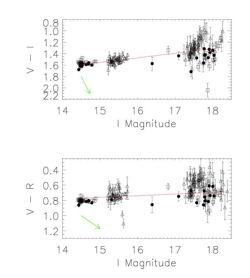
Figure 17: Here we show all the $V-I$ and $V-R$ data obtained at the USNO versus $I$ magnitude for 2001–2004 combined. Solid circles represent data from 2001/2002, squares represent data from 2002/2003, and diamonds represent data from 2003/2004. A straight line has been fit to the colors, while the short arrow represents the standard reddening that would be expected from IS dust grains for each color.

Combining the color data obtained over many seasons at the USNO, we illustrate the overall trend of color with brightness in Figure 17 . This confirms our impression that, out of eclipse, the star is about as red as it gets and shows relatively little color variation beyond what may be explained through star spots. As it enters (emerges from) eclipse the star gets bluer (redder) by 0.1–0.2 mag. Near minimum light there are substantial color variations; the star is sometimes at its bluest extreme, which is 0.3–0.4 mag bluer in $V-I$ than out-of-eclipse. However, sometimes it shows very little, if any, color effect.

4.2.3 Interpretation of the Color Data

A full explanation of the color data must await improved understanding of the details of this system, which will only come from an extensive phenomenological model currently being constructed (Winn et al. 2005, in prep). However, qualitative explanations for the observed trends can be proposed based on a few simple arguments. These lead to a set of questions that need to be addressed, and they suggest further observations that may clarify the situation.

Basically, blue colors indicate either the importance of wavelength-dependent scattering, such as from small grains or molecules, or the presence of a hotter component in the system, or both. It is likely that there is a hotter component in the system, since the currently invisible companion to the K7 star is known to be more luminous, as discussed above. All models of pre-main-sequence contraction indicate that the more massive star in a coeval pair is also more luminous and hotter, so it is reasonable to suppose that the currently invisible component of this system is also bluer than the K7 star. However, since the system was never substantially brighter in the past, even when both stars were visible, it is also true that this invisible component cannot be much more massive, luminous, or hotter than the K7 star. In fact, the lack of detectable change of spectral type during minimum means there is little other than K6 or K7 light in the system, as far as a stellar component.

The original interpretation proposed for the color variation by Herbst et al. (2002) is that near minimum light, we see the system primarily or only by reflected light and that some small grains are involved in the reflection. This is supported by the increased polarization detected near minimum light by Agol et al. (2004). The current data show, however, that there is almost certainly not a single color to which the star moves during eclipse, but rather that there is a great deal of real variability, some or all of which is phase dependent. Therefore, it cannot simply be that all of the light of the system is coming from distant, scattered radiation.

In particular, we are impressed by the relative peak in blueness that occurs near phase zero in the color-phase plots (Fig. 15 and 18). This is the time when the hotter, currently invisible, star is closest to the edge of the occulting cloud. We propose that the blue peak at this phase may be caused by this fact. We are apparently seeing a very small amount of either transmitted light or increased importance in the reflected component due to the light of this star, or, perhaps, the extension of a hot, circumstellar nebula associated with it, above the obscuring wall. In any event, we tentatively attribute the central peak in blue color and the phase-dependent variations around it as due to the orbital motion of a slightly bluer component (than the K7 star) relative to the edge of the occulting disk and, perhaps, relative to the principal scatterers.

The blue peaks associated with phases $\pm$0.17 in 2001/2002 are an entirely new feature of the light of this system revealed by the intensive color monitoring at CTIO during that season and deserve some explanation. We find it interesting, as noted above, that they seem to correlate with a distinct change in slope that occurs in the decline (rise) in magnitude during late ingress (early egress).

One problem in interpreting these data is that we do not yet know how sharp the occulting edge of the cloud is. Let us suppose, for the purposes of this qualitative study, that the edge is very sharp. In that case, we can identify the change of slope in decline (rise) rate as the point where the photosphere has just been completely covered (has first appeared). The fact that the color peaks blue at that point indicates that the blue light is closely associated with the photosphere, arising just above it. We suggest, therefore, that the light in this system contains a hotter component associated with an extended chromosphere or corona of the K7 star (and possibly its invisible companion as well). We have no idea whether the physical nature of this is a scaled-up solar-like chromosphere, a magnetically channeled accretion column, or something else. But the color evidence suggests an extended hotter, dense, optically thick zone located close to the photosphere of the K7 star. The persistence of the bluing of the light curve shows that it must be extended on a length scale comparable to a stellar radius.

An alternative model is that one is seeing a peculiar scattering effect just as the star enters (emerges) from full eclipse. One could imagine, for example, that strongly forward scattered light might glance off the top of an occulting disk providing a bluish “glint” at these phases. This would require, of course, wavelength-dependent scattering and, therefore, some component other than the obscuring cloud (which produces no reddening of the transmitted light). If wavelength-dependent reflection is heavily involved here, then there should be some dramatic increases in polarization during these phases. It would definitely be interesting to extend the polarization study of Agol et al. (2004) to a wider variety of phases. It will also be important to continue to monitor the color during these phases in future eclipses, hopefully including the $U$ band with larger telescopes, which will give important information on the nature of the scattering or the temperature of the emission zone.

5 Conclusions

The light curve of the remarkable system KH 15D continues to evolve, evidently as a result of an obscuring screen moving across the orbit of a binary. A periodogram analysis of our data indicates that the photometric period is in excellent agreement with the spectroscopic period. Analysis of the data collected outside of eclipse suggests that the visible star has a rotation period of $\sim$9.6 days. This conclusion is in accord with the predicted rotation period, which is derived from the measured $v\thinspace$sin$(i)$ (6.9 km s^-1) and taking sin$(i)$ $\approx$ 1.

Interpretation of the color information leads us to believe that some extended blue emission is revealed in the colors as the currently visible star goes into or comes out of eclipse. The eclipse length is now greater than half the orbital period of the system and continues to evolve, expanding at a rate that is $\sim$2 days year^-1. Continued photometric monitoring will help to further constrain the models. This object will clearly provide us with the opportunity to learn about disk evolution, the circumstellar environment of young stars, and the possibility of planet formation. Thus, we strongly encourage continued monitoring before it disappears!

Appendix A Appendix: $v\thinspace$sin$(i)$ Results

In order to determine the $v\thinspace$sin$(i)$ of the visible star in the KH 15D system, the UVES/VLT spectra (Hamilton et al. 2003) were revisited. First, a K7 V model spectrum was produced using a temperature of 4000 K, a log($g$) = 3.5 ($g$ in cgs units), and a macroturbulence value of 0. The template was then artificially broadened to resemble that of a higher velocity star by convolving it with a rotation profile that was generated from a theoretical model, and including a macroturbulence value of 2 km s^-1. This was accomplished by using an IDL code and various values of $v\thinspace$sin$(i)$ believed to span the range within which the $v\thinspace$sin$(i)$ of the visible K7 star is expected to be found.

Each broadened spectrum was then cross-correlated against the original narrow-lined template, and the FWHM of the peak of the cross-correlation function was measured. A plot of the FWHM values versus $v\thinspace$sin$(i)$ – a calibration curve – was produced by fitting a second-order polynomial function to the data. The 29 Nov. 2001 spectrum was then cross-correlated against the narrow-lined template and the FWHM value of the cross-correlation peak was measured. This value was determined to be 0.489. The polynomial fit to the calibration curve was evaluated at this FWHM value to obtain a $v\thinspace$sin$(i)$ = 6.9 $\pm$ 0.3 km s^-1 for the K7 star. The uncertainty was determined by first broadening our template spectrum to the value of 6.9 km s^-1. We then performed a Monte Carlo test where noise, appropriate to that which is found in the UVES/VLT spectrum, was added to the broadened template. This broadened, noisy template was then cross-correlated against the narrow-lined model spectrum. The FWHM of the peak of the cross-correlation function was measured for each test, and the standard deviation of these values provided us with our estimated uncertainty.

Table 1: Contributing Observatories for the 1995–2004 Seasons.

Observatory	Aperture	CCD Parameters	Filters	Dates Observed (UT)
VVO	0.6 m	0.5K $\times$ 0.5K, 0.6$\arcsec$ pix-1	$I$	27 Oct 1995 – 25 Mar 1998
VVO	0.6 m	1K $\times$ 1K, 0.6$\arcsec$ pix-1	$I$	10 Dec 1998 – 16 Mar 2004
ESO	2.2 m	8K $\times$ 8K, 0.238$\arcsec$ pix-1	$I$	30 Dec 2000 – 1 Mar 2001
CTIO	1.0 m	2K $\times$ 2K, 0.3$\arcsec$ pix-1	$V,I_{J}$	22 Aug 2001 – 18 Apr 2002
MMO	1.5 m	2K $\times$ 0.8K, 0.26$\arcsec$ pix-1	$I$	12 Sept 2001 – 18 Mar 2004
USNO	1.3 m	2K $\times$ 4K, 0.6$\arcsec$ pix-1	$V,R,I$	28 Nov 2001 – 3 Apr 2002
USNO	1.0 m	1K $\times$ 1K, 0.68$\arcsec$ pix-1	$B,V,R,I$	11 Nov 2002 – 30 Apr 2003
USNO	1.0 m	1K $\times$ 1K, 0.68$\arcsec$ pix-1	$V,R,I$	23 Dec 2003 – 12 Mar 2004
KPNO	0.9 m	2K $\times$ 2K, 0.6$\arcsec$ pix-1	$U,B,V,R,I$	1 – 22 Dec 2001
WISE	1.0 m	1K $\times$ 1K, 0.7$\arcsec$ pix-1	$I$	2 – 22 Dec 2001
Tenagra	0.81 m	1K $\times$ 1K, 0.87$\arcsec$ pix-1	$I$	2 Nov 2002 – 4 Apr 2004
KAIT	0.76 m	0.5K $\times$ 0.5K, 0.8$\arcsec$ pix-1	$I$	20 Sept 2002 – 30 Mar 2003
Teide	0.82 m	1K $\times$ 1K, 0.432$\arcsec$ pix-1	$I$	28 Sept 2002 – 28 Mar 2003
Konkoly	1.0 m	1K $\times$ 1K, 0.33$\arcsec$ pix-1	$I$	1 Oct 2002 – 2 Mar 2003

Table 2: Photometry Parameters for the 2002–2004 Seasons.

Observatory	Aperture Radius	Inner Sky Radius	Width
	in Pixels	in Pixels	in Pixels
VVO	7 (4.2$\arcsec$)	10 (6.0$\arcsec$)	5 (3.0$\arcsec$)
MMO	10 (2.6$\arcsec$)	11 (2.86$\arcsec$)	5 (1.3$\arcsec$)
USNO	4.5 (3.06$\arcsec$)	6.5 (4.42$\arcsec$)	2 (1.36$\arcsec$)
Tenagra	3 (2.61$\arcsec$)	5 (4.35$\arcsec$)	2 (1.74$\arcsec$)
KAIT	3 (2.4$\arcsec$)	5 (3.2$\arcsec$)	2 (1.6$\arcsec$)
Teide	2.5 (1.1$\arcsec$)	20 (8.6$\arcsec$)	8 (3.5$\arcsec$)
Konkoly	12 (3.96$\arcsec$)	15 (4.95$\arcsec$)	5 (1.65$\arcsec$)

Table 3: Adopted $UBVRI$ magnitudes and 1$\sigma$ uncertainties for the 7 Comparison Stars.

Star	$U$	$B$	$V$	$R$	$I$
A	14.401 $\pm$ 0.022	14.115 $\pm$ 0.021	13.368 $\pm$ 0.020	12.952 $\pm$ 0.020	12.548 $\pm$ 0.021
B	13.514 $\pm$ 0.022	13.341 $\pm$ 0.021	12.624 $\pm$ 0.020	12.196 $\pm$ 0.020	11.734 $\pm$ 0.021
C	13.563 $\pm$ 0.022	13.566 $\pm$ 0.021	12.969 $\pm$ 0.020	12.617 $\pm$ 0.020	12.240 $\pm$ 0.021
D	15.808 $\pm$ 0.028	15.921 $\pm$ 0.022	15.013 $\pm$ 0.020	14.328 $\pm$ 0.021	13.645 $\pm$ 0.021
E	15.803 $\pm$ 0.028	15.004 $\pm$ 0.022	13.885 $\pm$ 0.020	13.211 $\pm$ 0.021	12.614 $\pm$ 0.021
F	15.319 $\pm$ 0.024	14.745 $\pm$ 0.021	13.869 $\pm$ 0.020	13.375 $\pm$ 0.021	12.902 $\pm$ 0.021
G	16.842 $\pm$ 0.041	15.642 $\pm$ 0.022	14.230 $\pm$ 0.020	13.350 $\pm$ 0.021	12.479 $\pm$ 0.021

Table 4: $I$ Magnitudes and 1$\sigma$ uncertainties for Additional Comparison Stars.

	2001/2002	2002/2003	2003/2004
16D	14.303 $\pm$ 0.001	14.304 $\pm$ 0.001	14.302 $\pm$ 0.002
17D	15.085 $\pm$ 0.001	15.098 $\pm$ 0.002	15.158 $\pm$ 0.003
21D	15.023 $\pm$ 0.001	14.991 $\pm$ 0.002	15.006 $\pm$ 0.003
27D	13.783 $\pm$ 0.001	13.785 $\pm$ 0.001	13.794 $\pm$ 0.002
31D	14.423 $\pm$ 0.001	14.426 $\pm$ 0.001	14.411 $\pm$ 0.002

Table 5: Comparison Stars for 1995–2000 VVO Data.

Observing Season	Comparison Stars
1995/1996	16D, 31D
1996/1997	16D, 31D
1997/1998	27D, 31D
1998/1999	A, B, C, F
1999/2000	A, B, C, F, G
2000/2001	A, B, C, F

Table 6: Photometric Measurements of KH 15D.

Julian Date	$I$	$\sigma$	Observatory
2450017.8375	14.449	0.011	VVO
2450021.7443	14.521	0.024	VVO
2450026.7416	17.132	0.074	VVO
2450028.6983	14.687	0.014	VVO
2450028.8949	14.435	0.015	VVO
2450031.7696	14.014	0.007	VVO
2450039.7466	14.562	0.010	VVO
2450054.6473	14.466	0.009	VVO
2450056.7206	14.466	0.007	VVO
2450056.8106	14.457	0.009	VVO

Table 7: Color Measurements of KH 15D.

$V-I$	$\sigma$	$I$	$\sigma$	Avg. JD	Observatory
1.619	0.037	14.475	0.024	2452237.7643	USNO
1.582	0.024	14.525	0.018	2452241.8421	USNO
1.416	0.064	18.061	0.037	2452261.8464	KPNO
1.379	0.040	17.833	0.026	2452262.8831	KPNO
1.516	0.047	17.601	0.031	2452263.8295	KPNO
1.565	0.039	16.739	0.023	2452264.8739	KPNO
1.584	0.013	14.695	0.009	2452266.7740	USNO
1.621	0.014	14.519	0.008	2452269.8189	USNO
1.680	0.025	14.435	0.021	2452279.6966	USNO
1.716	0.091	17.427	0.073	2452306.8015	USNO

Table 8: Phases Corresponding to Outside of Eclipse.

Season	Phases
1995/1996	0.20–0.80
1996/1997	0.20–0.80
1997/1998	0.20–0.80
1998/1999	0.25–0.75
1999/2000	0.25–0.75
2000/2001	0.25–0.75
2001/2002	0.30–0.70
2002/2003	0.30–0.70
2003/2004	0.35–0.65

Table 9: Detected Periods Outside of Eclipse.

Season	Observatory	Period (d)	Power
2001/2002	CTIO	9.613, 7.953	14.6, 11.9
2003/2004	Tenagra	9.619	8.7

Figure 3: The light curve of KH 15D during 2001/2002 as observed from CTIO. Individual measurements are plotted. Variability out-of-eclipse is evident, in addition to changes in the shape of egress from eclipse to eclipse. Note the amplitude of the central reversal during this season.

Figure 4: Data obtained at different observatories on the same Julian Dates out-of-eclipse during 2002/2003. The key to the symbols is as follows: diamonds = VVO, triangles = USNO, Xs = MMO, squares = Tenagra, asterisks = KAIT, open circles = Teide.

Figure 5: The number of times an observatory’s measurement differed from the calculated nightly mean out-of-eclipse during 2002/2003.

Figure 6: Data obtained at different observatories on the same Julian Dates in deep eclipse during 2002/2003. The key to the symbols is the same as in Fig. 5: diamonds = VVO, triangles = USNO, Xs = MMO, squares = Tenagra, asterisks = KAIT, stars = Konkoly, open circles = Teide.

Figure 7: The number of times an observatory’s measurement differed from the calculated nightly mean in deep eclipse during 2002/2003.

Figure 8: Light curves from both the 2002/2003 and 2003/2004 seasons. The nightly means per observatory are plotted except when rapid changes in the brightness are occurring.

Figure 9: The light curves of KH 15D over a nine-year period. Mean $I$ magnitudes per observatory are plotted. The data span from 1995/1996, the first season of observation at VVO, to the most recent observing campaign of 2003/2004. There appears to be a linear relationship between depth and time.

Figure 11: Power spectrum of all the data during 1995–2004. The strongest peak occurs at a period of 48.37 days. The other four strong peaks occur at 42.71, 45.32, 51.78, and 55.84 days, respectively.

Figure 13: Power spectra of the out-of-eclipse data obtained at CTIO during the 2001/2002 season and the out-of-eclipse data obtained at Tenagra during the 2003/2004 season. Each spectrum shows a significant period of $\sim$9.6 days.

Figure 14: $V-I_{J}$ color obtained with the CTIO/Yale 1 m telescope during 2001/2002. The solid line represents the approximate beginning of ingress, whereas the dashed line represents the approximate end of egress. The color becomes dramatically bluer during ingress, and redder during egress, while it appears to be variable throughout the deepest part of the eclipse.

Figure 15: The data from Fig. 14 are shown here, phased with the 48.37 day period. In this figure, the arrows designate the approximate midpoints of ingress and egress, as well as where $I$ = 16.25 mag. The color becomes dramatically bluer during ingress, and redder during egress, while it appears to be variable throughout the deepest part of the eclipse.

Figure 16: Color data obtained out-of-eclipse during the 2002/2003 observing season at the USNO, Flagstaff Station versus phase. The star appears to be irregularly variable in all colors out-of-eclipse.

Figure 18: Here we show all the $V-I$ and $V-R$ data obtained at the USNO versus phase for 2001–2003. Solid circles represent the $V-I$ data and squares represent the $V-R$ data. The trends seen in the CTIO colors are also seen here.

References

- Agol et al. (2004) Agol, E., Barth, A. J., Wolf, S., & Charbonneau, D. 2004, ApJ, 600, 781
- Badalian & Erastova (1970) Badalian, H. S., & Erastova, L. K. 1970, Astron. Tsirk, 591, 4
- Barge & Viton (2003) Barge, P., & Viton, M. 2003, ApJ, 593, L117
- Chiang & Murray-Clay (2004) Chiang, E. I., & Murray-Clay, R. A. 2004, ApJ, 607, 913
- Deming, Charbonneau, & Harrington (2004) Deming, D., Charbonneau, D., & Harrington, J. 2004, ApJ, 601, L87
- DePoy et al. (2003) DePoy, D. L., et al., 2003, in Proc. SPIE Vol. 4841, “Instrument Design and Performance for Optical/Infrared Ground-Based Telescopes,” ed. M. Iye & A. Moorwood, p. 827
- Flaccomio et al. (1999) Flaccomio, E., Micela, G., Sciortino, S., Favata, F., Corbally, C., & Tomaney, A. 1999, A&A, 345, 521
- Grinin & Tambovtseva (2003) Grinin, V. P., & Tambovtseva, L. V. 2003, Astronomy Letters, 28, 601
- Hamilton et al. (2001) Hamilton, C. M., Herbst, W., Ferro, A. J., & Shih, C. 2001, ApJ, 554, L201
- Hamilton et al. (2003) Hamilton, C. M., Herbst, W., Mundt, R., Bailer-Jones, C. A. L., & Johns-Krull, C. M. 2003, ApJ, 591, L45
- Herbig (1954) Herbig, G. 1954, ApJ, 119, 483
- Herbst et al. (2002) Herbst, W., et al. 2002, PASP, 114, 1167
- Herbst & Shevchenko (1998) Herbst, W. & Shevchenko, V. V. 1998, BAAS, 30, 1361
- Horne & Baliunas (1986) Horne, J. H., & Baliunas, S. L. 1986, ApJ, 302, 757
- Hut (1981) Hut, P. 1981, A&A, 99, 126
- Johnson et al. (2004) Johnson, J. A., Marcy, G. W., Hamilton, C. M., Herbst, W., & Johns-Krull, C. M. 2004, AJ, 128, 1265
- Johnson & Winn (2004) Johnson, J. A., & Winn, J. N. 2004, AJ, 127, 2344
- Johnson et al. (2005) Johnson, J. A., Winn, J. N., Rampazzi, F., Barbieri, C., Mito, H., Tarusawa, K., Tsvetkov, M., Borisova, A., & Meusinger, H. 2005, AJ, 129, 1978
- Kearns et al. (1997) Kearns, K. E., Eaton, N. L., Herbst, W., & Mazzurco, C. J. 1997, AJ, 114, 1098
- Kearns & Herbst (1998) Kearns, K. E., & Herbst, W. 1998, AJ, 116, 261
- Kukarkin et al. (1972) Kukarkin, B. V., Kholopov, P. N., Kukarkina, N. P., & Perova, N. B. 1972, IBVS, 717, 1
- Lamm et al. (2004) Lamm, M. H., Bailer-Jones, C. A. L., Mundt, R., Herbst, W., & Scholz, A. 2004, A&A, 417, 557
- Lamm et al. (2005) Lamm, M. H., Mundt, R., Bailer-Jones, C. A. L., and Herbst, W. 2005, A&A, 430, 1005
- Landolt (1992) Landolt, A. U. 1992, AJ, 104, 372
- Li et al. (2003) Li, W., Filippenko, A. V., Chornock, R., & Jha, S. 2003, PASP, 115, 844
- Park et al. (2000) Park, B., Sung, H., Bessell, M. S., & Kang, Y. 2000, AJ, 120, 894
- Scargle (1982) Scargle, J. D. 1982, ApJ, 263, 835
- Stetson (1990) Stetson, P. B. 1990, PASP, 102, 932
- Tokunaga et al. (2004) Tokunaga, A. T., et al. 2004, ApJ, 601, L91
- Vasilevskis, Sanders, & Balz (1965) Vasilevskis, S., Sanders, W. L., & Balz, A. G. A. 1965, AJ, 70, 797
- Walker (1956) Walker, M. F. 1956, ApJS, 2, 365
- Winn et al. (2003) Winn, J. N., Garnavich, P. M., Stanek, K. Z., & Sasselov, D. D. 2003, ApJ, 593, L121
- Winn et al. (2004) Winn, J. N., Holman, M. J., Johnson, J. A., Stanek, K. Z., & Garnavich, P. 2004, ApJ, 603, L45
- Winn et al. (2005) Winn, J. N., et al. 2005, in preparation
- Worek (1996) Worek, T. F. 1996, PASP, 108, 962
- Zahn (1977) Zahn, J. P. 1977, A&A57, 383