Multi-frequency analysis of neutralino dark matter annihilations in the Coma cluster

We study the astrophysical implications of neutralino dark matter annihilations in galaxy clusters, with a specific application to the Coma cluster. We first address the determination of the dark halo models for Coma, starting from structure formation models and observational data, and we discuss in detail the role of sub-halos. We then perform a thorough analysis of the transport and diffusion properties of neutralino annihilation products, and investigate the resulting multi-frequency signals, from radio to gamma-ray frequencies. We also study other relevant astrophysical effects of neutralino annihilations, like the DM-induced Sunyaev-Zel’dovich effect and the intracluster gas heating. As for the particle physics setup, we adopt a two-fold approach, resorting both to model-independent bottom-up scenarios and to benchmark, GUT-motivated frameworks. We show that the Coma radio-halo data (the spectrum and the surface brightness) can be nicely fitted by the neutralino-induced signal for peculiar particle physics models and for magnetic field values, which we outline in detail. Fitting the radio data and moving to higher frequencies, we find that the multi-frequency spectral energy distributions are typically dim at EUV and X-ray frequencies (with respect to the data), but show a non-negligible gamma-ray emission, depending on the amplitude of the Coma magnetic field. A simultaneous fit to the radio, EUV and HXR data is not possible without violating the gamma-ray EGRET upper limit. The best-fit particle physics models yields substantial heating of the intracluster gas, but not sufficient energy injection as to explain the quenching of cooling flows in the innermost region of clusters. Due to the specific multi-frequency features of the DM-induced spectral energy distribution in Coma, we find that supersymmetric models can be significantly and optimally constrained either in the gamma-rays or at radio and microwave frequencies.

1 Introduction

Most of the matter content of the universe is in form of dark matter, whose presence is indicated by several astrophysical evidences (e.g., gravitational lensing, galaxy rotation curves, galaxy clusters masses) but whose nature is still elusive. On the cosmological side, the most recent results of observational cosmology, i.e. WMAP vs. distant SN Ia, indicate that the matter content of the universe is $\Omega_{m}h^{2}=0.135^{+0.008}_{-0.009}$ with a baryon density of $\Omega_{b}h^{2}=0.0224\pm 0.0009$ (Spergel et al. (2003)). The combination of the available data on large scale structures (Ly-$\alpha$ forest analysis of the SDSS, the SDSS galaxy clustering) with the latest SNe and with the 1-st year WMAP CMB anisotropies can improve the determination of the cosmological parameters (Seljak, et al. (2004)) and hence allow us to set a concordance cosmological model.
We refer, in this paper, to a flat $\Lambda$CDM cosmology with parameters chosen according to the global best fitting results derived in Seljak, et al. (2004) (see their Table 1, third column): we assume, in fact, that the present matter energy density is $\Omega_{m}=0.281$, that the Hubble constant in units of 100 km s^-1 Mpc^-1 is $h=0.71$, that the present mean energy density in baryons is $\Omega_{b}=0.0233/h^{2}$, with the only other significant extra matter term in cold dark matter $\Omega_{CDM}=\Omega_{m}-\Omega_{b}$, that our Universe has a flat geometry and a cosmological constant $\Lambda$, i.e. $\Omega_{\Lambda}=1-\Omega_{m}$, and, finally, that the primordial power spectrum is scale invariant and is normalized to the value $\sigma_{8}=0.897$. This choice sets our framework, but it is not actually crucial for any of the results presented in the paper, which can be easily rescaled in case of a re-assessment of best-fit values of the cosmological parameters, and in particular of the value of $\Omega_{CDM}$ (the present concordance cosmological model, while widely used, has been also criticized and questioned in the light of still unexplored systematics, see, e.g., Myers et al. (2003); Sadat et al. (2005); Lieu & Mittaz (2005); Copi et al. (2003))

The Coma cluster has been the first astrophysical laboratory for dark matter (DM) since the analysis of F. Zwicky (Zwicky (1933)). In this respect, we can consider the Coma cluster as an astrophysical benchmark case-study for DM. Modern observations have led to an increasingly sophisticated exploration of the DM distribution in the universe, now confirmed to be a dominant component (relative to the baryonic material) over scales ranging from those of galaxy halos to that of the particle horizon.

The nature of DM is not yet known and several detection techniques have been used so far. Obviously, direct detection is the cleanest and most decisive discriminant (see e.g. Munoz (2003) for a review). However, it would be interesting if astronomical techniques were to reveal some of the fundamental properties of DM particles. In fact, if DM is supposed to consist of fundamental particles which are weakly interacting, then their own interaction will lead to a number of astrophysical signatures (e.g., high-energy gamma-rays, electrons and positrons, protons and neutrinos and hence by their emission/interaction properties) indicative of their nature and composition.

These facts provide the basic motivations for our study, which is aimed to: i) describe the multi-wavelength signals of the presence of DM through the emission features of the secondary products of neutralino annihilation. These signals are of non-thermal nature and cover the entire electro-magnetic spectrum, from radio to gamma-ray frequencies; ii) indicate the best frequency windows where it will be possible to catch physical indications for the nature of DM; iii) apply this analysis to the largest bound containers of DM in the universe, i.e. galaxy clusters. We shall focus here on the case of the Coma cluster, a particularly rich and suitable laboratory for which an extended observational database is at hand.

1.1 The fundamental physics framework

Several candidates have been proposed as fundamental DM constituents, ranging from axions to light, MeV DM, from KK particles, branons, primordial BHs, mirror matter to supersymmetric WIMPs (see, e.g., Baltz, (2004), Bertone et al. (2004), and Bergstrom (2000) for recent reviews). In this paper we will assume that the main DM constituent is the lightest neutralino of the minimal supersymmetric extension of the Standard Model (MSSM). Although no experimental evidence in favor of supersymmetry has shown up to date, several theoretical motivations indicate that the MSSM is one of the best bets for new physics beyond the Standard Model. Intriguingly enough, and contrary to the majority of other particle physics candidates for DM, supersymmetry can unambiguously manifest itself in future accelerator experiments. Furthermore, provided neutralinos are stable and are the lightest supersymmetric particles, next generation direct detection experiments feature good chances to explore most of the neutralino-proton scattering cross section range predicted by supersymmetry.

A long standing issue in phenomenological studies of low-energy supersymmetry is traced to the parameterization of the supersymmetry breaking terms (see Chung et al. (2003) for a recent review). In this respect, two somehow complementary attitudes have been pursued. On the one hand, one can appeal to a (set of) underlying high energy principles to constrain the form of supersymmetry breaking term, possibly at some high energy (often at a grand unification) scale (see e.g. Baer et al. (2000)). The low energy setup is then derived through the renormalization group evolution of the supersymmetry breaking parameters down to the electroweak scale. Alternatively, one can directly face the most general possible low energy realization of the MSSM, and try to figure out whether general properties of supersymmetry phenomenology can be derived (see e.g. Profumo and Yaguna (2004)).

In this paper we will resort to both approaches. We will show that the final state products of neutralino pair annihilations show relatively few spectral patterns, and that any supersymmetric configuration can be thought as an interpolation among the extreme cases we shall consider here. The huge number of free parameters of the general MSSM are therefore effectively decoupled, and the only relevant physical properties are the final state products of neutralino pair annihilations, and the mass of the neutralino itself. We will indicate this first strategy as a bottom-up approach (see Sect.4.1 for details).

Since most phenomenological studies have been so far based on GUT-motivated models, and a wealth of results on accelerator physics, direct and indirect detection has accumulated within these frameworks, we decided to work out here, as well, the astrophysical consequences, for the system under consideration, of a few benchmark models. The latter have been chosen among the minimal supergravity (mSUGRA) models indicated in Battaglia et al. (2003) with the criterion of exemplifying the widest range of possibilities within that particular theoretical setup (see Sect.3.2 for details).

1.2 The astrophysical framework

To make our study quantitative, we will compare the predictions of the above mentioned neutralino models with the observational set-up of the Coma cluster, which represents the largest available observational database for a galaxy cluster. The total mass of Coma found within $10h^{-1}$ Mpc from its center is $M_{<10h^{-1}Mpc}\approx 1.65\times 10^{15}M_{\odot}$ (Geller et al. (1999)). The assumption of hydrostatic equilibrium of the thermal intra-cluster gas in Coma provides a complementary estimate of its total mass enclosed in the radius $r$. A value $M\approx 1.85\times 10^{15}M_{\odot}$ within $5h^{-1}_{50}$ Mpc from the cluster center has been obtained from X-ray data (Hughes (1989)).
X-ray observations of Coma also yield detailed information about the thermal electrons population. We know that the hot thermal electrons are at a temperature $k_{B}T_{e}=8.2\pm 0.4$ keV (Arnaud et al. (2001)) and have a central density $n_{0}=(3.42\pm 0.047)\,h_{70}^{1/2}\times 10^{-3}$ cm^-3, with a spatial distribution fitted by a $\beta$-model, $n(r)=n_{0}(1+r^{2}/r_{c}^{2})^{-3\beta/2}$, with parameters $r_{c}=10.5^{\prime}\pm 0.6^{\prime}$ and $\beta\approx 0.75$ (Briel et al. (1992)). Assuming spherical symmetry and the previous parameter values, the optical depth of the thermal gas in Coma is $\tau_{th}\simeq 5.54\times 10^{-3}$ and the pressure due to the thermal electron population is $P_{th}\simeq 2.80\cdot 10^{-2}$ keV cm^-3. The hot intra-cluster gas produces also a thermal SZ effect (Sunyaev & Zel’dovich (1972, 1980); see Birkinshaw (1999) for a general review) which has been observed over a wide frequency range, from $32$ to $245$ GHz (see DePetris et al. (2003) and references therein).
Beyond the presence of DM and thermal gas, Coma also shows hints for the presence of relativistic particles in its atmosphere. The main evidence for the presence of a non-thermal population of relativistic electrons comes from the observation of the diffuse radio halo at frequencies $\nu_{r}\sim 30MHz-5GHz$ (Deiss et al. (1997); Thierbach et al. (2003)). The radio halo spectrum can be fitted by a power-law spectrum $J_{\nu}\sim\nu^{-1.35}$ in the range $30$ MHz-$1.4$ GHz with a further steepening of the spectrum at higher radio frequencies. The radio halo of Coma has an extension of $R_{h}\approx 0.9h_{70}^{-1}$ Mpc, and its surface brightness is quite flat in the inner 20 arcmin with a radial decline at larger angular distances (e.g., Colafrancesco et al. (2005)).
Other diffuse non-thermal emissions have been reported for Coma (as well as for a few other clusters) in the extreme UV (EUV) and in the hard X-ray (HXR) energy bands. The Coma flux observed in the $65-245$ eV band (Lieu et al. (1996)) is $\sim 36\%$ above the expected flux from the thermal bremsstrahlung emission of the $k_{B}T\approx 8.2$ keV IC gas (Ensslin et al. (1998)) and it can be modeled with a power-law spectrum with an approximately constant slope $\approx 1.75$, in different spatial regions (Lieu et al. (1999), Ensslin et al. (1999), Bowyer et al. (2004)). The EUV excess in Coma has been unambiguously detected and it does not depend much on the data analysis procedure. The integrated flux in the energy band $0.13-0.18$ keV is $F_{EUV}\approx(4.1\pm 0.4)\cdot 10^{-12}$ erg cm^-2s^-1  (Bowyer et al. (2004)). According to the most recent analysis of the EUVE data (Bowyer et al. (2004)), the EUV excess seems to be spatially concentrated in the inner region ($\theta\ \raise-2.0pt\hbox{\hbox to0.0pt{\hbox{$\sim$}\hss}\raise 5.0pt\hbox{$<$}\ }15-20$ arcmin) of Coma (see also Bonamente et al. (2003)). The nature of this excess is not definitely determined since both thermal and non-thermal models are able to reproduce the observed EUV flux. However, the analysis of Bowyer et al. (2004) seems to favour a non-thermal origin of the EUV excess in Coma generated by an additional population of secondary electrons. A soft X-ray (SXR) excess (in the energy range $\approx 0.1-0.245$ keV) has been also detected in the outer region ($20^{\prime}<\theta<90^{\prime}$) of Coma (Bonamente et al. (2003); Finoguenov et al. (2003)). The spectral features of this SXR excess seem to be more consistent with a thermal nature of the SXR emission, while a non-thermal model is not able to reproduce accurately the SXR data (e.g., Bonamente et al. (2003)). The SXR emission from the outskirts of Coma has been fitted in a scenario in which the thermal gas at $k_{B}T_{e}\sim 0.2$ keV with $\sim 0.1$ solar abundance (see, e.g. Finoguenov et al. (2003) who identify the warm gas with a WHIM component) resides in the low-density filaments predicted to form around clusters as a result of the evolution of the large-scale web-like structure of the universe (see Bonamente et al. (2003)). It has been noticed, however, that the WHIM component cannot reproduce, by itself, the Coma SXR excess because it would produce a SXR emission by far lower (see Mittaz et al. (2004)), and thus one is forced to assume a large amount of warm gas in the outskirts of Coma. Thus, it seems that the available EUV and SXR data indicate (at least) two different electron populations: a non-thermal one, likely yielding the centrally concentrated EUV excess and a thermal (likely warm) one, providing the peripherically located SXR excess. In this paper, we will compare our models with the EUV excess only, which is intimately related to Coma being spatially concentrated towards the inner region of the cluster.
There is also evidence of a hard X-ray (HXR) emission observed towards the direction of Coma with the BeppoSAX-PDS (Fusco-Femiano et al. (1999), Fusco-Femiano et al. (2004)) and with the ROSSI-XTE experiments (Rephaeli et al. (1999)). Both these measurements indicate an excess over the thermal emission which amounts to $F_{(20-80)keV}=(1.5\pm 0.5)\cdot 10^{-11}$ erg s^-1 cm^-2 (Fusco-Femiano et al. (2004)). It must be mentioned, for the sake of completeness, that the HXR excess of Coma is still controversial (see Rossetti and Molendi (2004)), but, for the aim of our discussion, it could at worst be regarded as an upper limit. The nature of the HXR emission of Coma is not yet fully understood.
Finally, a gamma-ray upper limit of $F(>100MeV)\approx 3.2\times 10^{-8}$ pho cm^-2 has been derived for Coma from EGRET observations (Sreekumar et al. (1996), Reimer et al. (2004)).

The current evidence for the radio-halo emission features of Coma has been interpreted as synchrotron emission from a population of primary relativistic electrons which are subject to a continuous re-acceleration process supposedly triggered by merging shock and/or intracluster turbulence (e.g., Brunetti et al. (2004)). The EUV and HXR emission excesses are currently interpreted as Inverse Compton scattering (ICS) emission from either primary or secondary electrons. Alternative modeling has been proposed in terms of suprathermal electron bremsstrahlung emission for the HXR emission of Coma (see Ensslin et al. (1999); Kempner & Sarazin (2000), see also Petrosian (2001) for a critical discussion) and in this case the EUV emission should be produced either by a different relativistic electron population or by a warm thermal population both concentrated towards the cluster center. Lastly, models in which the EUV and HXR emission can be reproduced by synchrotron emission from the interaction of Ultra High Energy cosmic rays and/or photons (Timokhin et al. (2003); Inoue et al. (2005)) have also been presented. The situation is far from being completely clear and several problems still stand on both the observational and theoretical sides of the issue.

Since DM is abundantly present in Coma and relativistic particles are among the main annihilation products, we explore here the effect of DM annihilation on the multi-frequency spectral energy distribution (SED) of Coma. The plan of the paper is the following. We discuss in Sect. 2 the DM halo models for the Coma cluster, the set of best fitting parameters for the DM distribution, and the role of sub-halos. The annihilation features of neutralinos and the main annihilation products are discussed in Sect. 3. The multi-frequency signals of DM annihilation are presented and discussed in details in Sect. 4 and 5, while the details of the transport and diffusion properties of the secondary particles are described in the Appendix A, together with the derivation of the equilibrium spectrum of relativistic particles in Coma. The conclusions of our analysis and the outline for forthcoming astrophysical searches for DM signals in galaxy clusters are presented in the final Sect.6.

2 A $\Lambda$CDM model for the Coma cluster

To describe the DM halo profile of the Coma cluster we refer, as a general setup, to the $\Lambda$CDM model for structure formation, implementing results of galaxy cluster formation obtained from N-body simulations. Free parameters are fitted against the available dynamical information and are compared to the predictions of this scheme. Substructures will play a major role when we will discuss the predictions for signals of DM annihilations. In this respect, the picture derived from simulations is less clean and, hence, we will describe in details our set of assumptions.

2.1 The dark matter halo profile

To describe the DM halo profile of the Coma cluster we consider the limit in which the mean DM distribution in Coma can be regarded as spherically symmetric and represented by the parametric radial density profile:

$$\rho(r)=\rho^{\prime}g(r/a)\,.$$ (1)

Two schemes are adopted to choose the function $g(x)$ introduced here. In the first one, we assume that $g(x)$ can be directly inferred as the function setting the universal shape of DM halos found in numerical N-body simulations of hierarchical clustering. We are assuming, hence, that the DM profile is essentially unaltered from the stage preceding the baryon collapse, which is – strictly speaking – the picture provided by the simulations for the present-day cluster morphology. A few forms for the universal DM profile have been proposed in the literature: we implement here the non-singular form (which we label as N04 profile) extrapolated by Navarro et al. (2004):

$$g_{N04}(x)=\exp[-2/\alpha(x^{\alpha}-1)]\;\;\;\;{\rm with}\;\;\;\;\alpha\simeq 0.17\;,$$ (2)

and the shape with a mild singularity towards its center proposed by Diemand et al. (2005) (labeled here as D05 profile):

$$g_{D05}(x)=\frac{1}{x^{\gamma}(1+x)^{3-\gamma}}\;\;\;\;{\rm with}\;\;\;\;\gamma\simeq 1.2\;.$$ (3)

The other extreme scheme is a picture in which the baryon infall induces a large transfer of angular momentum between the luminous and the dark components of the cosmic structure, with significant modification of the shape of the DM profile in its inner region. According to a recent model (El-Zant et al. (2001)), baryons might sink in the central part of DM halos after getting clumped into dense gas clouds, with the halo density profile in the final configuration found to be described by a profile (labeled here as B profile) with a large core radius (see, e.g., Burkert (1995)):

$$g_{B}(x)=\frac{1}{(1+x)\,(1+x^{2})}\;.$$ (4)

Once the shape of the DM profile is chosen, the radial density profile in Eq. (1) is fully specified by two parameters: the length-scale $a$ and the normalization parameter $\rho^{\prime}$. It is, however, useful to describe the density profile model by other two parameters, i.e., its virial mass $M_{vir}$ and concentration parameter $c_{vir}$. For the latter parameter, we adopt here the definition by Bullock et al. (2001). We introduce the virial radius $R_{vir}$ of a halo of mass $M_{vir}$ as the radius within which the mean density of the halo is equal to the virial overdensity $\Delta_{vir}$ times the mean background density $\bar{\rho}=\Omega_{m}\rho_{c}$:

$$M_{vir}\equiv{4\pi\over 3}\Delta_{vir}\bar{\rho}\,R_{vir}^{3}.$$ (5)

We assume here that the virial overdensity can be approximated by the expression (see  Bryan & Norman (1998)), appropriate for a flat cosmology,

$$\Delta_{vir}\simeq{\frac{(18\pi^{2}+82x-39x^{2})}{1-x}}\;,$$ (6)

with $x\equiv\Omega_{m}(z)-1$. In our cosmological setup we find at $z=0$, $\Delta_{vir}\simeq 343$ (we refer to Colafrancesco et al. (1994), Colafrancesco et al. (1997) for a general derivation of the virial overdensity in different cosmological models). The concentration parameter is then defined as

$$c_{vir}=\frac{R_{vir}}{r_{-2}}\equiv\frac{R_{vir}}{x_{-2}\,a}\;,$$ (7)

with $r_{-2}$ the radius at which the effective logarithmic slope of the profile is $-2$. We find that $x_{-2}=1$ for the N04 profile (see Eq. 2), $x_{-2}=2-\gamma$ for D05 profile (see Eq. 3), and $x_{-2}\simeq 1.52$ for the Burkert profile (see Eq. 4).

Since the first numerical results with large statistics became available (Navarro et al. (1997)), it has been realized that, at any given redshift, there is a strong correlation between $c_{vir}$ and $M_{vir}$, with larger concentrations found in lighter halos. This trend may be intuitively explained by the fact that mean overdensities in halos should be correlated with the mean background densities at the time of collapse, and in the hierarchical structure formation model small objects form first, when the Universe was indeed denser. The correlation between $c_{vir}$ and $M_{vir}$ is relevant in our context at two levels: i) when discussing the mean density profile of Coma and, ii) when including substructures. Hence, we will review this relevant issue here and we will apply it to the present case of Coma. Bullock et al. (2001) proposed a model to describe this correlation, improving on the toy model originally outlined in Navarro et al. (1997). A collapse redshift $z_{c}$ is assigned, on average, to each halo of mass $M$ at the epoch $z$ through the relation $M_{\star}(z_{c})\equiv FM$. Here it is postulated that a fixed fraction $F$ of $M$ (following Wechsler et al. (2001) we choose $F=0.015$) corresponds to the typical collapsing mass $M_{\star}$, as defined implicitly by $\sigma\left(M_{\star}(z)\right)=\delta_{sc}(z)$, with $\delta_{sc}$ being the critical overdensity required for collapse in the spherical model and $\sigma(M)$ being the present-day rms density fluctuation in spheres containing a mean mass $M$ (see, e.g., Peebles (1980)). An expression for $\delta_{sc}$ is given, e.g., in Eke et al. (1996). The rms fluctuation $\sigma(M)$ is related to the fluctuation power spectrum $P(k)$ (see e.g. Peebles (1993)) by

$$\sigma^{2}(M)\equiv\int d^{3}k\;\tilde{W}^{2}(k\,R)\,P(k)\,,$$ (8)

where $\tilde{W}$ is the top-hat window function on the scale $R^{3}=3M/4\pi\bar{\rho}$ with $\bar{\rho}$ the mean (proper) matter density, i.e. $\bar{\rho}=\Omega_{m}\rho_{c}$ with $\rho_{c}$ the critical density. The power spectrum $P(k)$ is parametrized as $P(k)\propto k^{n}T^{2}(k)$ in terms of the primordial power-spectrum shape $\propto k^{n}$ and of the transfer function $T^{2}(k)$ associated to the specific DM scenario. We fix the primordial spectral index $n=1$ and we take the transfer function $T^{2}(k)$ given by Bardeen et al. (1986) for an adiabatic CDM model, with the shape parameter modified to include baryonic matter according to the prescription in, e.g. Peacock (1999) (see their eqs.15.84 and 15.85) and introducing a multiplicative exponential cutoff at large $k$ corresponding to the free-streaming scale for WIMPs (Hofmann et al. 2001, Chen et al. 2001, Green et al. 2005, Diemand et al. (2005)). The spectrum $P(k)$ is normalized to the value $\sigma_{8}=0.897$ as was quoted above.

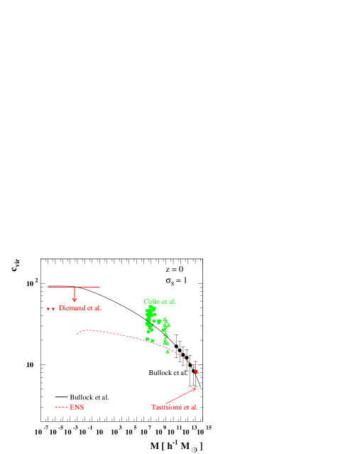
Figure 1: The dependence of $c_{vir}$ on the halo mass $M$, at $z=0$, as in the Bullock et al. toy model (solid line) and in the ENS toy model (dashed line); predictions are compared to a few sets of simulation results in different mass ranges. A flat, vacuum-dominated cosmology with $\Omega_{M}=0.3$, $\Omega_{\Lambda}=0.7$, $h=0.7$ and $\sigma_{8}=1$ is assumed here.

The toy model of Bullock et al. (2001) prescribes a one to one correspondence between the density of the Universe at the collapse redshift $z_{c}$ of the DM halo and a characteristic density of the halo at the redshift $z$; it follows that, on average, the concentration parameter is given by

$$c_{vir}(M,z)=K\frac{1+z_{c}}{1+z}=\frac{c_{vir}(M,z=0)}{(1+z)}\;,$$ (9)

with $K$ being a constant (i.e. independent of $M$ and cosmology) to be fitted to the results of the N-body simulations. We plot in Fig. 1 the dependence of $c_{vir}$ on the halo mass $M$, at $z=0$, according to the toy model of Bullock et al. (2001) as extrapolated down to the free-streaming mass scale for DM halos made of WIMPs, i.e. around $10^{-6}\,M_{\odot}{\ }$ (see Hofmann et al. 2001, Chen et al. 2001, Green et al. 2005, Diemand et al. (2005)). The predictions are compared to the results of a few sets of N-body simulations: we use “data” points and relative error bars from Bullock et al. (2001) (representing a binning in mass of results for a large sample of simulated halos; in each mass bin, the marker and the error bars correspond, respectively, to the peak and the 68% width in the $c_{vir}$ distribution) to determine the parameter $K$. The same value will be used to infer the mean $c_{vir}$ predicted in our cosmological setup. Other “datasets” refer actually to different values of $\sigma_{8}$ and different redshifts $z$ ($z=26$ for the two minihalos fitted in Fig. 2 of Diemand et al. (2005) and for the upper bound in the range up to $10\,M_{\odot}{\ }$ quoted in the same paper; $z=3$ for the sample from Colin et al. (2004)) and have been extrapolated, consistently with our prescriptions, to $z=0$ and $\sigma_{8}=1$. Since small objects tend to collapse all at the same redshift, the dependence on mass of the concentration parameters flattens at small masses; the mean asymptotic value we find is slightly larger than the typical values found in Diemand et al. (2005), but it is still consistent with that analysis.

An alternative toy-model to describe the relation between $c_{vir}$ and $M$ has been discussed by Eke, Navarro and Steinmetz (Eke et al. (2001), hereafter ENS model). The relation they propose has a similar scaling in $z$, but with a different definition of the collapse redshift $z_{c}$ and a milder dependence of $c_{vir}$ on $M$. In our notation, they define $z_{c}$ through the equation

$$D(z_{c})\sigma_{\rm eff}(M_{p})={1\over C_{\sigma}}$$ (10)

where $D(z)$ represents the linear theory growth factor, and $\sigma_{\rm eff}$ is an ‘effective’ amplitude of the power spectrum on scale $M$:

$$\sigma_{\rm eff}(M)=\sigma(M)\,\left(-\frac{d\ln(\sigma)}{d\ln(M)}(M)\right)=-\frac{d\sigma}{dM}M$$ (11)

which modulates $\sigma(M)$ and makes $z_{c}$ dependent on both the amplitude and on the shape of the power spectrum, rather than just on the amplitude, as in the toy model of Bullock et al. (2001). Finally, in Eq. (10), $M_{p}$ is assumed to be the mass of the halo contained within the radius at which the circular velocity reaches its maximum, while $C_{\sigma}$ is a free parameter (independent of $M$ and cosmology) which we will fit again to the “data” set in Bullock et al. (2001). With such a definition of $z_{c}$ it follows that, on average, $c_{vir}$ can be expressed as:

$$c_{vir}(M,z)=\left(\frac{\Delta_{vir}(z_{c})\,\Omega_{M}(z)}{\Delta_{vir}(z)\,\Omega_{M}(z_{c})}\right)^{1/3}\frac{1+z_{c}}{1+z}\;.$$ (12)

As shown in Fig. 1, the dependence of $c_{vir}$ on $M$ given by Eq.(12) above is weaker than that obtained in the Bullock et al. (2001) toy-model, with a significant mismatch in the extrapolation already with respect to the sample from Colin et al. (2004) and an even larger mismatch in the low mass end. Moreover, the extrapolation breaks down when the logarithmic derivative of the $\sigma(M)$ becomes very small, in the regime when $P(k)$ scales as $k^{-3}$. Note also that predictions in this model are rather sensitive to the specific spectrum $P(k)$ assumed (in particular the form in the public release of the ENS numerical code gives slightly larger values of $c_{vir}$ in its low mass end, around a value $c_{vir}\approx 40$ (we checked that implementing our fitting function for the power spectrum, we recover our trend).

2.2 Fitting the halo parameters of Coma

For a given shape of the halo profile we make a fit of the parameters $M_{vir}$ and $c_{vir}$ against the available dynamical constraints for Coma. We consider two bounds on the total mass of the cluster at large radii, as inferred with techniques largely insensitive to the details of the mass profile in its inner region. In Geller et al. (1999), a total mass

$$M(r<10\;{\rm h}^{-1}\,{\rm Mpc})=(1.65\pm 0.41)\,10^{15}\;{\rm h}^{-1}\,M_{\odot}\;$$ (13)

is derived mapping the caustics in redshift space of galaxies infalling in Coma on nearly radial orbits. Several authors derived mass budgets for Coma using optical data and applying the virial theorem, or using X-ray data and assuming hydrostatic equilibrium. We consider the bound derived by Hughes (1989), cross-correlating such techniques:

$$M(r<5\;{\rm h}_{50}^{-1}\,{\rm Mpc})=(1.85\pm 0.25)\,10^{15}\;{\rm h}_{50}^{-1}\,M_{\odot}\;,$$ (14)

where $h_{50}$ is the Hubble constant in units of 50 km s^-1 Mpc^-1.

In our discussion some information on the inner shape of the mass profile in Coma is also important: we implement here the constraint that can derived by studying the velocity moments of a given tracer population in the cluster. As the most reliable observable quantity one can consider the projection along the line of sight of the radial velocity dispersion of the population; under the assumption of spherical symmetry and without bulk rotation, this is related to the total mass profile $M(r)$ by the expression (Binney & Mamon (1982); Lokas & Mamon (2003)):

$$\sigma_{\rm los}^{2}(R) = \frac{2G}{I(R)}\int_{R}^{\infty}\,{\rm d}r^{\prime}\ \nu(r^{\prime})M(r^{\prime})(r^{\prime})^{2\beta-2}$$ (15)

$$\times\int_{R}^{r^{\prime}}\,{\rm d}r\left(1-\beta\frac{R^{2}}{r^{2}}\right)\frac{r^{-2\beta+1}}{\sqrt{r^{2}-R^{2}}}\ ,$$

where $\nu(r)$ is the density profile of the tracer population and $I(R)$ represents its surface density at the projected radius $R$. In the derivation of Eq. (15), a constant-over-radius anisotropy parameter $\beta$ defined as

$$\beta\equiv 1-\frac{\sigma_{\theta}^{2}(r)}{\sigma_{r}^{2}(r)}\;,$$ (16)

has been assumed with $\sigma_{r}^{2}$ and $\sigma_{\theta}^{2}$ being, respectively, the radial and tangential velocity dispersion ($\beta=1$ denotes the case of purely radial orbits, $\beta=0$ that of system with isotropic velocity dispersion, while $\beta\rightarrow-\infty$ labels circular orbits). Following Lokas & Mamon (2003), we take as tracer population that of the E-S0 galaxies, whose line of sight velocity dispersion has been mapped, according to Gaussian distribution, in nine radial bins from $4^{\prime}$ out to $190^{\prime}$ (see Fig. 3 in Lokas & Mamon (2003)), and whose density profile can be described by the fitting function:

$$\nu(r)\propto\frac{1}{(r/r_{\rm S})(1+r/r_{\rm S})^{2}}\ ,$$ (17)

with $r_{\rm S}=7\hbox{$.\mkern-4.0mu^{\prime}$}05$. Constraints to the DM profile are obtained through its contribution to $M(r)$, in which we include the terms due to spiral and E-S0 galaxies (each one with the appropriate density profile normalized to the observed luminosity through an appropriate mass-to-light ratio), and the gas component (as inferred from the X-ray surface brightness distribution) whose number density profile can be described by the fitting function:

$$n(r)=n_{0}\left[1+\left(\frac{r}{r_{\rm c}}\right)^{2}\right]^{-1.5\;b}\,,$$ (18)

with $n_{0}=3.42\times 10^{-3}$ cm^-3, $r_{\rm c}=10\hbox{$.\mkern-4.0mu^{\prime}$}5$ and $b=0.75$ (Briel et al. (1992)).

To compare a model with such datasets, we build a reduced $\chi^{2}$-like variable of the form:

$$\chi^{2}_{r} = \frac{1}{2}\bigg{[}\frac{1}{2}\sum_{i=1}^{2}\frac{\left(M(r<r_{i})-M_{i}\right)^{2}}{(\Delta M_{i})^{2}}$$ (19)

$$+\frac{1}{9}\sum_{j=1}^{9}\frac{\left(\sigma_{\rm los}(R_{j})-\sigma_{\rm los}^{j}\right)^{2}}{(\Delta\sigma_{\rm los}^{j})^{2}}\bigg{]}$$

where the index $i$ in the first sum runs over the constraints given in Eqs. (13) and (14), while, in the second sum, we include the nine radial bins over which the line of sight velocity dispersion of E-S0 galaxies and its standard deviation has been estimated. Weight factors have been added to give the same statistical weight to each of the two classes of constraints, see, e.g., Dehnen & Binney (1998) where an analogous procedure has been adopted.

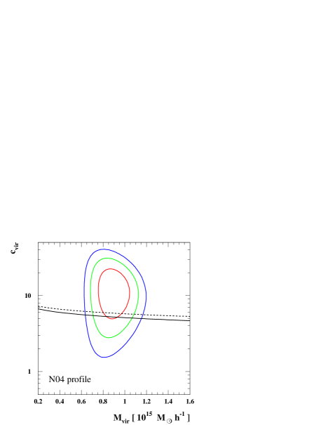
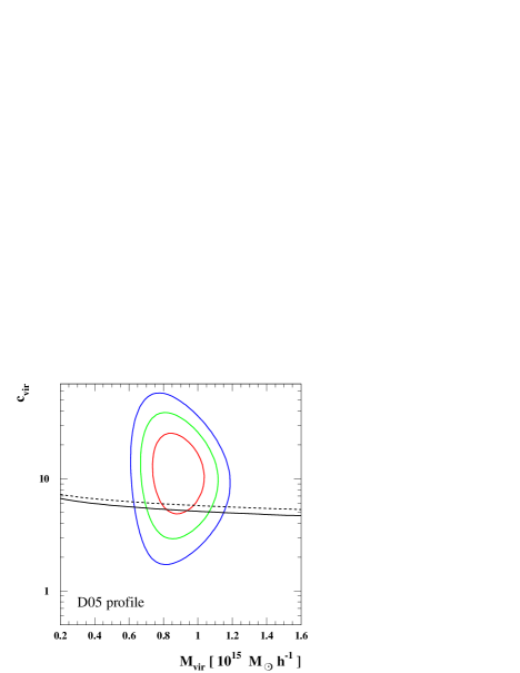
Figure 2: We show the 1 $\sigma$, 2 $\sigma$ and 3 $\sigma$ contours as derived from the $\chi^{2}_{r}$ variable in eq.(19), for the Navarro et al. halo profile, Eq. (2), (upper panel) and for the Diemand et al. halo profile, Eq. (3) (lower panel). Also shown are mean values for the correlation between $M_{vir}$ and $c_{vir}$ as in the toy models of Bullock et al. (2001) (solid line) and that of Eke et al. (2001) (dashed line).

Nonetheless, we have derived in Fig. 2 the 1 $\sigma$, 2 $\sigma$ and 3 $\sigma$ contours in the $(M_{vir},\;c_{vir})$ plane for the Navarro et al. halo profile (Eq. (2) and for the Diemand et al. halo profile (Eq. 3). In Fig. 3 we show the analogous contours for the Burkert profile (Eq. (4)). In all these cases we have performed the fit of the line-of-sight radial velocity dispersion of E-S0 galaxies assuming that this system has an isotropic velocity dispersion, i.e. we have taken $\beta=0$. Best fitting values are found at $M_{vir}\simeq 0.9\cdot 10^{15}M_{\odot}{\ }h^{-1}$ and $c_{vir}\simeq 10$ (that we consider, hence, as reference values in the following analysis), not too far from the mean value expected from models sketching the correlation between these two parameters in the $\Lambda$CDM picture. We show in Figs. 2 and 3 the predictions of such correlation in the models of Bullock et al. (solid line) and of Eke et al. (2001) (dashed line).

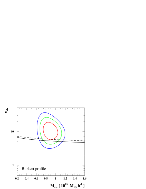
Figure 3: We show here the 1 $\sigma$, 2 $\sigma$ and 3 $\sigma$ contours as derived from the $\chi^{2}_{r}$ variable introduced in the text, for the Burkert profile, Eq. (4).

2.3 Substructures in the Coma cluster

Since the astrophysical signals produced by WIMP pair annihilation scale with the square of the WIMP density, any local overdensity does play a role (see e.g. Bergstrom et al. (1998) and references therein). To discuss substructures in the Coma cluster, analogously to the general picture introduced above for DM halos, we label a subhalo through its virial mass $M_{s}$ and its concentration parameter $c_{s}$ (or equivalently a typical density and length scale, $\rho^{\prime}_{s}$ and $a_{s}$). The subhalo profile shape is considered here to be spherical and of the same form as for the parent halo. Finally, as for the mean DM density profile, the distribution of subhalos in Coma is taken to be spherically symmetric. The subhalo number density probability distribution can then be fully specified through $M_{s}$, $c_{s}$ and the radial coordinate for the subhalo position $r$. To our purposes, it is sufficient to consider the simplified case when the dependence on these three parameters can be factorized, i.e.:

$$\frac{dn_{s}}{dr^{3}\,dM_{s}\,dc_{s}}=p_{s}(r)\,\frac{dn_{s}}{dM_{s}}(M_{s})\,{\cal{P}}_{s}(c_{s})\;.$$ (20)

Here we have introduced a subhalo mass function, independent of radius, which is assumed to be of the form:

$$\frac{dn_{s}}{dM_{s}}=\frac{A(M_{vir})}{M_{s}^{1.9}}\exp{\left[-\left(\frac{M_{s}}{M_{cut}}\right)^{-2/3}\right]}\;,$$ (21)

Diemand et al. (2005) where $M_{cut}$ is the free streaming cutoff mass (Hofmann et al. 2001, Chen et al. 2001, Green et al. 2005, Diemand et al. (2005)), while the normalization $A(M_{vir})$ is derived imposing that the total mass in subhalos is a fraction $f_{s}$ of the total virial mass $M_{vir}$ of the parent halo, i.e.

$$\int_{M_{cut}}^{M_{vir}}dM_{s}\frac{dn_{s}}{dM_{s}}M_{s}=f_{s}M_{vir}\;.$$ (22)

According to Diemand et al. (2005), $f_{s}$ is about 50% for a Milky Way size halo, and we will assume that the same holds for Coma. The quantity ${\cal{P}}_{s}(c_{s})$ is a log-normal distribution in concentration parameters around a mean value set by the substructure mass; the trend linking the mean $c_{s}$ to $M_{s}$ is expected to be analogous to that sketched above for parent halos with the Bullock et al. or ENS toy models, except that, on average, substructures collapsed in higher density environments and suffered tidal stripping. Both of these effects go in the direction of driving larger concentrations, as observed in the numerical simulation of Bullock et al. (2001), where it is shown that, on average and for $M\sim 5\cdot 10^{11}M_{\odot}{\ }$ objects, the concentration parameter in subhalos is found to be a factor of $\approx 1.5$ larger than for halos. We make here the simplified ansazt:

$$\langle c_{s}(M_{s})\rangle=F_{s}\langle c_{vir}(M_{vir})\rangle\;\;\;\;{\rm with}\;\;\;\;M_{s}=M_{vir}\;,$$ (23)

where, for simplicity, we assume that the enhancement factor $F_{s}$ does not depend on $M_{s}$. Following again Bullock et al. (2001), the $1\sigma$ deviation $\Delta(\log_{10}c_{s})$ around the mean in the log-normal distribution ${\cal{P}}_{s}(c_{s})$, is assumed to be independent of $M_{s}$ and of cosmology, and to be, numerically, $\Delta(\log_{10}c_{s})=0.14$.
Finally, we have to specify the spatial distribution of substructures within the cluster. Numerical simulations, tracing tidal stripping, find radial distributions which are significantly less concentrated than that of the smooth DM component. This radial bias is introduced here assuming that:

$$p_{s}(r)\propto g(r/a^{\prime})\;,$$ (24)

with $g$ being the same functional form introduced above for the parent halo, but with $a^{\prime}$ much larger than the length scale $a$ found for Coma. Following Nagai & Kravtsov (2005), we fix $a^{\prime}/a\simeq 7$. Since the fraction $f_{s}$ of DM in subhalos refers to structures within the virial radius, the normalization of $p_{s}(r)$ follows from the requirement

$$4\pi\int_{0}^{R_{vir}}r^{2}p_{s}(r)=1\;.$$ (25)

3 Neutralino annihilations in Coma

3.1 Statistical properties

Having set the reference particle physics framework and specified the distribution of DM particles, we can now introduce the source function from neutralino pair annihilations. For any stable particle species $i$, generated promptly in the annihilation or produced in the decay and fragmentation processes of the annihilation yields, the source function $Q_{i}(r,E)$ gives the number of particles per unit time, energy and volume element produced locally in space:

$$Q_{i}(r,E)=\langle\sigma v\rangle_{0}\sum_{f}\frac{dN_{i}^{f}}{dE}(E)B_{f}\;{\cal N}_{\rm pairs}(r)\;,$$ (26)

where $\langle\sigma v\rangle_{0}$ is the neutralino annihilation rate at zero temperature. The sum is over all kinematically allowed annihilation final states $f$, each with a branching ratio $B_{f}$ and a spectral distribution $dN_{i}^{f}/dE$, and ${\cal N}_{\rm pairs}(r)$ is the number density of neutralino pairs at a given radius $r$ (i.e., the number of DM particles pairs per volume element squared). The particle physics framework sets the quantity $\langle\sigma v\rangle_{0}$ and the list of $B_{f}$. Since the neutralino is a Majorana fermion light fermion final states are suppressed, while – depending on mass and composition – the dominant channels are either those with heavy fermions or those with gauge and Higgs bosons. The spectral functions $dN_{i}^{f}/dE$ are inferred from the results of MonteCarlo codes, namely the Pythia (Sjöstrand 1994, (1995)) 6.154, as included in the DarkSUSY package (Gondolo et al. (2004)). Finally, ${\cal N}_{\rm pairs}(r)$ is obtained by summing the contribution from the smooth DM component, which we write here as the difference between the cumulative profile and the term that at a given radius is bound in subhalos, and the contributions from each subhalo, in the limit of unresolved substructures and in view of the fact that we consider only spherically averaged observables:

$${\cal N}_{\rm pairs}(r) = \bigg{[}\frac{\left(\rho^{\prime}g(r/a)-f_{s}\,M_{vir}\,p_{s}(r)\right)^{2}}{2\,M_{\chi}^{2}}$$ (27)

$$+p_{s}(r)\,\int dM_{s}\frac{dn_{s}}{dM_{s}}\int dc_{s}^{\,\prime}\;{\cal{P}}_{s}\left(c_{s}^{\,\prime}(M_{s})\right)$$

$$\times\int d^{3}r_{s}\;\frac{\left(\rho^{\prime}_{s}\,g(r_{s}/a_{s})\right)^{2}}{2\,M_{\chi}^{2}}\bigg{]}\;.$$

This quantity can be rewritten in the more compact form:

$${\cal N}_{\rm pairs}(r) = \frac{\bar{\rho}^{2}}{2\,M_{\chi}^{2}}\bigg{[}\frac{\left(\rho^{\prime}g(r/a)-f_{s}\,\tilde{\rho}_{s}\,g(r/{a^{\prime}})\right)^{2}}{\bar{\rho}^{2}}$$ (28)

$$+f_{s}\Delta^{2}\,\frac{\tilde{\rho}_{s}\,g(r/{a^{\prime}})}{\bar{\rho}}\bigg{]}\;,$$

where we have normalized densities to the present-day mean matter density in the Universe $\bar{\rho}$, and we have defined the quantity:

$$f_{s}\Delta^{2} \equiv \frac{\int dM_{s}\frac{dn_{s}}{dM_{s}}M_{s}\Delta_{M_{s}}^{2}(M_{s})}{M_{vir}}$$ (29)

$$= f_{s}\frac{\int dM_{s}\frac{dn_{s}}{dM_{s}}M_{s}\Delta_{M_{s}}^{2}(M_{s})}{\int dM_{s}\frac{dn_{s}}{dM_{s}}M_{s}}\;,$$ (30)

with

$$\Delta_{M_{s}}^{2}(M_{s})\equiv\frac{\Delta_{vir}(z)}{3}\,\int dc_{s}^{\,\prime}\;{\cal{P}}_{s}\left(c_{s}^{\,\prime}\right)\frac{I_{2}(c_{s}^{\,\prime}\,x_{-2})}{\left[I_{1}(c_{s}^{\,\prime}\,x_{-2})\right]^{2}}(c_{s}^{\,\prime}\,x_{-2})^{3}\;$$ (31)

and

$$I_{n}(x)=\int_{0}^{x}dy\,y^{2}\left[g(y)\right]^{n}\;.$$ (32)

Such definitions are useful since $\Delta_{M_{s}}^{2}$ gives the average enhancement in the source due to a subhalo of mass $M_{s}$, while $\Delta^{2}$ is the sum over all such contributions weighted over the subhalo mass function times mass. Finally, in Eq. (28) we have also introduced the quantity:

$$\tilde{\rho}_{s}\equiv\frac{M_{vir}}{4\,\pi\,(a^{\prime})^{3}I_{1}\left(R_{vir}/a^{\prime}\right)}\;.$$ (33)

In the limit in which the radial distribution of substructures traces the DM profile, i.e. $a^{\prime}=a$, $\tilde{\rho}_{s}$ becomes equal to the halo normalization parameter $\rho^{\prime}$.

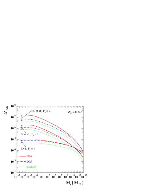
Figure 4: Scaling of the average enhancement in source functions due to a subhalo of mass $M_{s}$. We show result implementing the three halo profiles introduced, i.e. the N04, D05 and Burkert profile, the two toy models for the scaling of concentration parameter with mass, i.e. the Bullock et al. and the ENS, and two sample values of the ratio between concentration parameter in subhalos to concentration parameter in halos at equal mass $F_{s}$.

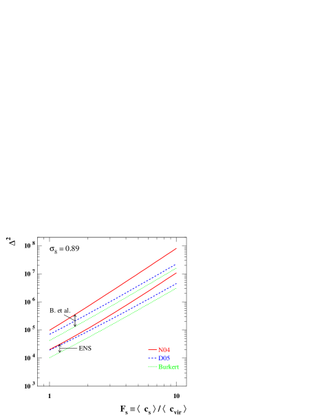
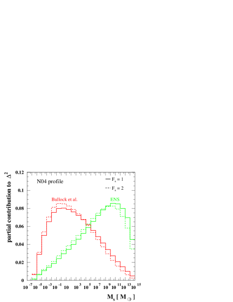
Figure 5: Left: scaling of the weighted enhancement in source functions due to subhalos versus the ratio between concentration parameter in subhalos to concentration parameter in halos at equal mass $F_{s}$. Results are shown the three halo profiles introduced, i.e. the N04, D05 and Burkert profile, the two toy models for the scaling of concentration parameter with mass, i.e. the Bullock et al. and the ENS. Right: fractional contribution per logarithmic interval in subhalo mass $M_{s}$ to $\Delta^{2}$ in four sample cases. A normalization of the fluctuation spectrum $\sigma_{8}=0.89$ is adopted.

We show in Fig. 4 the scaling of the average enhancement $\Delta_{M_{s}}^{2}$ in the source function versus the subhalo mass $M_{s}$. We have considered the three halo models introduced in the previous Section, i.e. the N04, D05 and Burkert profiles, for the two toy models describing the scaling of concentration parameter with mass, i.e. the Bullock et al. and the ENS schemes, as well as two sample values for the ratio $F_{s}$ between the average concentration parameter in subhalos and that in halos of equal mass. In each setup, going to smaller and smaller values of $M_{s}$, the average enhancement $\Delta_{M_{s}}^{2}$ increases and then flattens out at the mass scale below which all structures tend to collapse at the same epoch, and hence have equal concentration parameter.

In Fig. 5 we show the scaling of the weighted enhancement $\Delta^{2}$ in the source function due to subhalos versus the ratio between concentration parameter in subhalos to concentration parameter in halos at equal mass $F_{s}$; we give results for the usual set of halo profiles considered in our approach. Analogously to the enhancement for a fixed mass shown in the previous plot, $\Delta^{2}$ is very sensitive to the scaling of the concentration parameter and hence we find a sharp dependence of $\Delta^{2}$ on $F_{s}$. The fractional contribution per logarithmic interval in subhalo mass $M_{s}$ to $\Delta^{2}$ is also shown in Fig. 5 for four sample cases. Note that, although the factorization in the probability distribution for clumps in the radial coordinate and mass (plus the assumption that $F_{s}$ does not depend on mass) are a crude approximation, what we actually need in our discussion is $F_{s}$ and the radial distribution for subhalos at the peak of the distribution shown in Fig. 5: unfortunately we cannot read out this from numerical simulations.

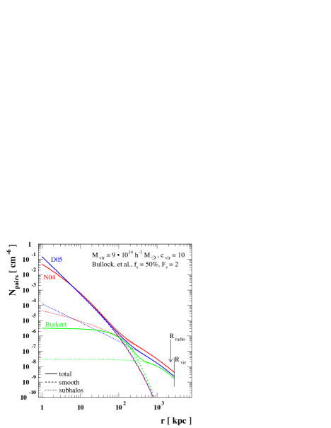
Figure 6: The number density of neutralino pairs (neutralino mass set to $M_{\chi}=100$ GeV) as a function distance for the center of Coma for the three halo profiles introduced, i.e. the N04, D05 and Burkert profile in their best fit model, and a sample configuration for the subhalo parameters.

Fig. 6 shows the number density of neutralino pairs (we set here the neutralino mass to $M_{\chi}=100$ GeV) as a function of the distance from the center of Coma for the three representative halo profiles introduced here, i.e. the N04, D05 and Burkert profile in their best fit model, and a sample configuration for the subhalo parameters. For the D05 and N04 profiles, the central enhancement increases the integrated source function by a factor $\approx 6$ with respect to the Burkert profile, but this takes place on such a small angular scale that from the observational point of view it is like adding a point source at the center of the cluster. The enhancement of the annihilation signals from subhalos comes instead from large radii. This means that the enhancement from subhalos largely influences the results when the neutralino source is extended. This is the case of galaxy clusters, and more specifically of the Coma cluster which is our target in this paper.

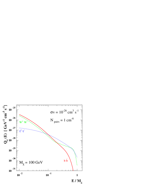
Figure 7: The spectral shape of the electron source function in case of three sample final states (see text for details.

3.2 Source functions spectral properties: generalities and supersymmetric benchmarks

The spectral properties of secondary products of DM annihilations depend only, prior to diffusion and energy losses, on the DM particle mass $M_{\chi}$ and on the branching ratio $BR(\chi\chi\rightarrow f)$ for the final state $f$ in the DM pair-annihilation. The DM particle physics model further sets the magnitude of the thermally averaged pair annihilation cross section times the relative DM particles velocity, $\langle\sigma v\rangle_{0}$ at $T=0$.

The range of neutralino masses and pair annihilation cross sections in the most general supersymmetric DM setup is extremely wide. Neutralinos as light as few GeV (see Bottino et al. (2003)) and as heavy as hundreds of TeV (see Profumo (2005)) can account for the observed CDM density through thermal production mechanisms, and essentially no constraints apply in the case of non-thermally produced neutralinos.

Turning to the viable range of neutralino pair annihilation cross sections, coannihilation processes do not allow us to set any lower bound, while on purely theoretical grounds a general upper limit on $\langle\sigma v\rangle_{0}\ \raise-2.0pt\hbox{\hbox to0.0pt{\hbox{$\sim$}\hss}\raise 5.0pt\hbox{$<$}\ }10^{-22}\left(\frac{M_{\chi}}{{\rm TeV}}\right)^{-2}{\rm cm}^{3}/{\rm s}$ has been recently set (Profumo (2005)). The only general argument which ties the relic abundance of a WIMP with its pair annihilation cross section is given by the naive relation

$$\Omega_{\chi}h^{2}\simeq{3\times 10^{-27}{\rm cm}^{3}/{\rm s}\over\langle\sigma v\rangle_{0}}$$ (34)

(see Jungman et al. (1995), Eq.3.4), which points at a fiducial value for $\langle\sigma v\rangle_{0}\simeq 3\times 10^{-26}{\rm cm}^{3}/{\rm s}$ for our choice of cosmological parameters. The above mentioned relation can be, however, badly violated in the general MSSM, or even within minimal setups, such as the minimal supergravity scenario (see Profumo (2005)).

Since third generation leptons and quarks Yukawa couplings are always much larger than those of the first two generations, and being the neutralino a Majorana fermion, the largest $BR(\chi\chi\rightarrow f)$ for annihilations into a fermion-antifermion pair are in most cases into the third generation final states $b\overline{b}$, $t\overline{t}$ and $\tau^{+}\tau^{-}$. In the context of supersymmetry, if the supersymmetric partners of the above mentioned fermions are not significantly different in mass, the $\tau^{+}\tau^{-}$ branching ratio will be suppressed, with respect to the $b\overline{b}$ branching ratio by a color factor equal to 1/3, plus a possible further Yukawa coupling suppression, since the two final states share the same $SU(2)$ quantum number assignment. Further, the fragmentation functions of third generation quarks are very similar, and give rise to what we will dub in the following as a “soft spectrum”. A second possibility, when kinematically allowed, is the pair annihilation into massive gauge bosons, $W^{+}W^{-}$ and $Z_{0}Z_{0}$. Again, the fragmentation functions for these two final states are mostly indistinguishable, and will be indicated as giving a “hard spectrum”. The occurrence of a non-negligible branching fraction into $\tau^{+}\tau^{-}$ or into light quarks will generally give raise to intermediate spectra between the ”hard” and ”soft” case.
Fig.7 shows the spectral shape of the electron source function in the case of the three sample final states $b\overline{b}$, $\tau^{+}\tau^{-}$ and $W^{+}W^{-}$ for $M_{\chi}=100$ GeV, and clarifies the previous discussion. In what follows we will therefore employ sample DM configurations making use of either soft ($b\overline{b}$) or hard ($W^{+}W^{-}$) spectra, keeping in mind that other possibilities would likely fall in between these two extrema.

In order to make a more stringent contact with supersymmetry phenomenology, we will however also resort to realistic benchmark SUSY models: by this we mean thoroughly defined SUSY setups which are fully consistent with accelerator and other phenomenological constraints, and which give a neutralino thermal relic abundance exactly matching the central cosmologically observed value. To this extent, we refer to the so-called minimal supergravity model (Goldberg 1983; Ellis et al. 1983, (1984)), perhaps one of the better studied paradigms of low-energy supersymmetry, which enables, moreover, a cross-comparison with numerous dedicated studies, ranging from colliders (Baer et al. (2003)) to DM searches (Edsjo et al. 2004, Baer et al. (2004)).

The assumptions of universality in the gaugino and in the scalar (masses and trilinear couplings) sectors remarkably reduce, in this model, the number of free parameters of the general soft SUSY breaking Lagrangian (Chung et al. (2003)) down to four continuous parameters ($m_{0},\ M_{1/2},A_{0},\tan\beta$) plus one sign (${\rm sign}(\mu)$). The mSUGRA parameter space producing a sufficiently low thermal neutralino relic abundance $\Omega_{\chi}h^{2}$ has been shown to be constrained to a handful of “regions” featuring effective $\Omega_{\chi}h^{2}$ suppression mechanisms (Ellis et al. (2003)). The latter are coannihilations of the neutralino with the next-to-lightest SUSY particle (“Coannihilation” region), rapid annihilations through $s$ channel Higgs exchanges (“Funnel” region), the occurrence of light enough neutralino and sfermions masses (“Bulk” region) and the presence of a non-negligible bino-higgsino mixing (“Focus Point” region).

With the idea of allowing a direct comparison with the existing research work in a wealth of complementary fields, we restrict ourselves to the “updated post-WMAP benchmarks for supersymmetry” proposed and studied by Battaglia et al. (2003). All of those setups are tuned so as to feature a neutralino thermal relic density giving exactly the central WMAP-estimated CDM density. As a preliminary step, we computed the electrons, neutrinos, gamma-rays and protons source spectra for all the 13 ${\bf A}^{\prime}$-${\bf M}^{\prime}$ models. Remarkably enough, although the SUSY particle spectrum is rather homogeneous throughout the mSUGRA parameter space, the resulting spectra exhibit at least three qualitatively different shapes, according to the dominant final state in neutralino pair annihilation processes. In particular, in the Bulk and Funnel regions the dominant final state is into $b\bar{b}$, and, with a sub-dominant variable contribution, $\tau^{+}\tau^{-}$. The latter channel is instead dominant, for kinematic reasons, in the stau Coannihilation region. Finally, a third, and last, possibility is a dominant gauge bosons final state, which is the case along the Focus Point region. In this respect, in the effort to reproduce all of the mentioned spectral modes, and to reflect every cosmologically viable mSUGRA region, we focused on the four models indicated in Table 1, a subset of the benchmarks of Battaglia et al. (2003) (to which we refer the reader for further details).

Model	$M_{1/2}$	$m_{0}$	$\tan\beta$	${\rm sign}(\mu)$	$m_{t}$
${\bf B}^{\prime}$ (Bulk)	250	57	10	$>0$	175
${\bf D}^{\prime}$ (Coann.)	525	101	10	$>0$	175
${\bf E}^{\prime}$ (Focus P.)	300	1653	10	$>0$	171
${\bf K}^{\prime}$ (Funnel)	1300	1070	46	$<0$	175

Table 1: The input parameters of the four mSUGRA benchmark models we consider here. The units for the mass parameters are GeV, and the universal trilinear coupling $A_{0}$ is set to 0 for all models (see Battaglia et al. (2003) for details).

Model	BR($b\bar{b}$)	BR($\tau^{+}\tau^{-}$)	BR($W^{+}W^{-}$)	BR($Z^{0}Z^{0}$)	$\langle\sigma v\rangle_{0}$
${\bf B}^{\prime}$ (Bulk)	74%	19%	4%	0%	$7.8\times 10^{-28}$
${\bf D}^{\prime}$ (Coann.)	21%	61%	0%	0%	$8.9\times 10^{-29}$
${\bf E}^{\prime}$ (Focus P.)	1%	0%	90%	8%	$1.7\times 10^{-26}$
${\bf K}^{\prime}$ (Funnel)	88%	11%	0%	0%	$1.1\times 10^{-26}$

Table 2: The branching ratios into various final states for the four mSUGRA benchmark models of tab. 1; in the last column we also indicate $\langle\sigma v\rangle_{0}$ in units of ${\rm cm}^{3}{\rm s}^{-1}$.

We collect in Table 2 the branching ratios for the final states of neutralino pair annihilations. In the last column of this table we also provide the thermally-averaged pair annihilation cross section times the relative velocity, at $T=0$, $\langle\sigma v\rangle_{0}$. Table 2 is an accurate guideline to interpret the resulting source spectra for the four benchmarks under consideration here, which are shown in Figs. 8 and 9. Fig.8 shows in particular the differential electron (left) and photon (right) yields per neutralino annihilation multiplied by $\langle\sigma v\rangle_{0}$, i.e. the source function $Q(r,E)$ divided by the number density of neutralino pairs ${\cal N}_{\rm pairs}(r)$ as a function of the particles’ kinetic energy. As mentioned above, the Bulk and Funnel cases are very similar between each other, though in the latter case one has a heavier spectrum and a larger value of $\langle\sigma v\rangle_{0}$. Fig.9 shows the same quantity for neutrinos and protons.

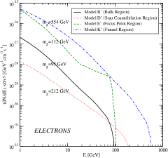
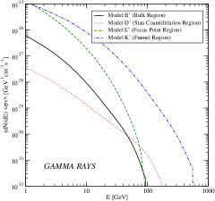
Figure 8: (Left): The electrons flux $(dN_{e}/dE)\langle\sigma v\rangle_{0}$ as a function of the electron energy. (Right): The gamma-rays flux $(dN_{\gamma}/dE)\langle\sigma v\rangle_{0}$ as a function of the photon energy.

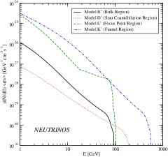
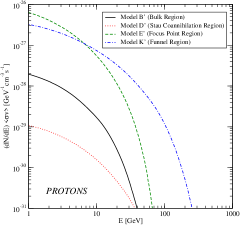
Figure 9: (Left): The neutrinos flux $(dN_{\nu}/dE)\langle\sigma v\rangle_{0}$ as a function of the neutrino energy. (Right): The protons flux $(dN_{p}/dE)\langle\sigma v\rangle_{0}$ as a function of the proton energy.

The products of the neutralino annihilation which are more relevant to our discussion are secondary electrons and pions. The secondary particles produced by neutralino annihilation are subject to various physical mechanisms: i) decay (which is especially fast for pions and muons); ii) energy losses which can be suffered by stable particles, like electrons and positrons; iii) spatial diffusion of these relativistic particles in the atmosphere of the cluster. Gamma-rays produced by neutral pion decay, $\pi^{0}\to\gamma\gamma$, generate most of the continuum spectrum at energies $E\ \raise-2.0pt\hbox{\hbox to0.0pt{\hbox{$\sim$}\hss}\raise 5.0pt\hbox{$>$}\ }1$ GeV and this emission is directly radiated since the $\pi^{0}\to\gamma\gamma$ e.m. decay is very fast. This gamma-ray emission is dominant at high energies, $\ \raise-2.0pt\hbox{\hbox to0.0pt{\hbox{$\sim$}\hss}\raise 5.0pt\hbox{$>$}\ }0.3-0.5$ of the neutralino mass, but needs to be complemented by other two emission mechanisms which produce gamma-rays at similar or slightly lower energies: these are the ICS and the bremsstrahlung emission by secondary electrons. We will discuss the full gamma-ray emission of Coma induced by DM annihilation in Sect. 4 below. Secondary electrons are produced through various prompt generation mechanisms and by the decay of charged pions (see, e.g., Colafrancesco & Mele (2001)). In fact, charged pions decay through $\pi^{\pm}\to\mu^{\pm}\nu_{\mu}(\bar{\nu}_{\mu})$, with $\mu^{\pm}\to e^{\pm}+\bar{\nu}_{\mu}(\nu_{\mu})+\nu_{e}(\bar{\nu}_{e})$ and produce $e^{\pm}$, muons and neutrinos. Electrons and positrons are produced abundantly by neutralino annihilation (see Fig. 8, left) and are subject to spatial diffusion and energy losses. Both spatial diffusion and energy losses contribute to determine the evolution of the source spectrum into the equilibrium spectrum of these particles, i.e. the quantity which will be used to determine the overall multi-wavelength emission induced by DM annihilation. The secondary electrons eventually produce radiation by synchrotron in the magnetized atmosphere of Coma, Inverse Compton Scattering of CMB (and other background) photons and bremsstrahlung with protons and ions in the atmosphere of the Coma cluster (see, e.g., Colafrancesco & Mele (2001) and Colafrancesco (2003, 2006) for a review). These secondary particles also produce heating of the intra-cluster gas by Coulomb collisions with the intra-cluster gas particles and SZ effect (see, e.g. Colafrancesco (2003), Colafrancesco (2006)). Other fundamental particles which might have astrophysical relevance are also produced in DM annihilation. Protons are produced in a smaller quantity with respect to $e^{\pm}$ (see Fig. 9, right), but do not loose energy appreciably during their lifetime while they can diffuse and be stored in the cluster atmosphere. These particles can, in principle, produce heating of the intra-cluster gas and $pp$ collisions providing, again, a source of secondary particles (pions, neutrinos, $e^{\pm}$, muons, …) in complete analogy with the secondary particle production by neutralino annihilation. Neutrinos are also produced in the process of neutralino annihilation (see Fig. 9, left) and propagate with almost no interaction with the matter of the cluster. However, the resulting flux from Coma is found to be unobservable by current experiments.

To summarize, the secondary products of neutralino annihilation which have the most relevant astrophysical impact onto the multi-frequency spectral energy distribution of DM halos are neutral pions and secondary electrons.

4 Neutralino-induced signals

A complete description of the emission features induced by DM must take, consistently, into account the diffusion and energy-loss properties of these secondary particles. These mechanisms are taken into account in the following diffusion equation (i.e. neglecting convection and re-acceleration effects):

$$\frac{\partial}{\partial t}\frac{dn_{e}}{dE} = \nabla\left[D(E,\@vec{x})\nabla\frac{dn_{e}}{dE}\right]+\frac{\partial}{\partial E}\left[b(E,\@vec{x})\frac{dn_{e}}{dE}\right]$$ (35)

$$+Q_{e}(E,\@vec{x})\;,$$

where $dn_{e}/dE$ is the equilibrium spectrum, $D(E,\@vec{x})$ is the diffusion coefficient, $b(E,\@vec{x})$ is the energy loss term and $Q_{e}(E,\@vec{x})$ is the source function. The analytical solution of this equation for the case of the DM source function is derived in the Appendix A.
In the limit in which electrons and positrons lose energy on a timescale much shorter than the timescale for spatial diffusion, i.e. the regime which applies to the case of galaxy clusters, the first term on the r.h.s. of Eq. (64) can be neglected, and the expression for equilibrium number density becomes:

$$\left({\frac{dn_{e}}{dE}}\right)_{nsd}\left(r,E\right)=\frac{1}{b(E)}\int_{E}^{M_{\chi}}dE^{\prime}\;Q_{e}(r,E^{\prime})\;,$$ (36)

(see the Appendix A for a general discussion of the role of spatial diffusion and of the regimes in which it is relevant).

The derivation of the full solution of the diffusion equation (Eq. 64) and the effects of diffusion and energy losses described in the Appendix A, set us in the position to discuss the multi-frequency emission produced by the DM (neutralino) component of the Coma cluster. We will present the overall DM-induced spectral energy distribution (hereafter SED) from low to high observing frequencies.

We describe here our reference setup for the numerical calculations. Our reference halo setup is the N04 profile and other parameters/choice of extrapolation schemes as in Fig. 6. We consider the predictions of two particle models, one with a branching ratio equal to 1 in $b\bar{b}$, i.e. a channel with a soft production spectrum, and the second one with a branching ratio equal to 1 into $W^{+}W^{-}$, i.e. a channel with hard spectrum. Since we have previously shown that diffusion is not relevant in a Coma-like cluster of galaxy, we neglect, in our numerical calculations, the spatial diffusion for electrons and positrons: this is the limit in which the radial dependence and frequency dependence can be factorized in the expression for the emissivity.

4.1 Radio emission

At radio frequencies, the DM-induced emission is dominated by the synchrotron radiation of the relativistic secondary electrons and positrons of energy $E=\gamma m_{e}c^{2}$, living in a magnetic field $B(r)$ and a background plasma with thermal electron density $n(r)$, and in the limit of frequency $\nu$ of the emitted photons much larger than the non-relativistic gyro-frequency $\nu_{0}=eB/(2\pi mc)\simeq 2.8B_{\mu}$ Hz and the plasma frequency $\nu_{p}=8980\left(n(r)/1cm^{-3}\right)^{1/2}$ Hz. Averaging over the directions of emission, the spontaneously emitted synchrotron power at the frequency $\nu$ is given by (Longair (1994)):

$$P_{\rm synch}\left(\nu,E,r\right)=\int_{0}^{\pi}d\theta\frac{\sin\theta}{2}2\pi\sqrt{3}r_{0}mc\nu_{0}\sin\theta F\left(x/\sin\theta\right)\;,$$ (37)

where we have introduced the classical electron radius $r_{0}=e^{2}/(mc^{2})=2.82\cdot 10^{-13}$ cm, and we have defined the quantities $x$ and $F$ as:

$$x\equiv\frac{2\nu}{3\nu_{0}\gamma^{2}}\left[1+\left(\frac{\gamma\nu_{p}}{\nu}\right)^{2}\right]^{3/2}\;,$$ (38)

and

$$F\left(t\right)\equiv t\int_{t}^{\infty}dzK_{5/3}(z)\simeq 1.25t^{1/3}\exp{(-t)}\left[648+t^{2}\right]^{1/12}\;.$$ (39)

Folding the synchrotron power with the spectral distribution of the equilibrium number density of electrons and positrons, we get the local emissivity at the frequency $\nu$:

$$j_{\rm synch}\left(\nu,r\right)=\int_{m_{e}}^{M_{\chi}}dE\,\left(\frac{dn_{e^{-}}}{dE}+\frac{dn_{e^{+}}}{dE}\right)P_{\rm synch}\left(\nu,E,r\right)\,.$$ (40)

This is the basic quantity we need in order to compare our predictions with the available data. In particular, we will compare our predictions with measurements of the integrated (over the whole Coma radio halo size) flux density spectrum:

$$S_{\rm synch}(\nu)=\int d^{3}r\,\frac{j_{\rm synch}\left(\nu,r\right)}{4\pi\,D_{\rm Coma}^{2}}\;,$$ (41)

where $D_{\rm Coma}$ is the luminosity distance of Coma, and with the azimuthally averaged surface brightness distribution at a given frequency and within a beam of angular size $\Delta\Omega$ (PSF):

$$I_{\rm synch}(\nu,\Theta,\Delta\Omega)=\int_{\Delta\Omega}d\Omega\int_{l.o.s.}dl\,\frac{j_{\rm synch}\left(\nu,l\right)}{4\pi}\;,$$ (42)

where the integral is performed along the line of sight (l.o.s.) $l$, within a cone of size $\Delta\Omega$ centered in a direction forming an angle $\Theta$ with the direction of the Coma center.

We started from the full dataset on the radio flux density spectrum (Thierbach et al. (2003)) and minimized the fit with respect to the WIMP mass (with the bound $M_{\chi}\geq 10$ GeV for the $b\bar{b}$ case, and mass above threshold for the $W^{+}W^{-}$ case), the strength of the magnetic field (with the bound $B_{\mu}\geq 1\mu G$) and the annihilation rate $\langle\sigma v\rangle_{0}$. The spectrum predicted by two models with the lowest values of $\chi^{2}_{r}$ are shown in Fig. 10. In both cases the best fit corresponds to the lowest neutralino mass allowed, since this is the configuration in which the fall-off of the flux density at the highest observed frequency tends to be better reproduced. For the same reason, the fit in the case of a soft spectrum is favored with respect to the one with a hard spectrum (we have checked that in case of $\tau^{+}\tau^{-}$ again does not give a bend-over in the spectrum where needed). The values of the annihilation rates required by the fit are fairly large: $\langle\sigma v\rangle_{0}=4.7\cdot 10^{-25}$ cm³ s^-1 for $b\bar{b}$ case, and about one order of magnitude smaller, $\langle\sigma v\rangle_{0}=8.8\cdot 10^{-26}$ cm³ s^-1, for the $W^{+}W^{-}$ case, despite the heavier neutralino mass, since the best fit values correspond to different values of the magnetic field of about $1.2\mu G$ and $8\mu G$, respectively.

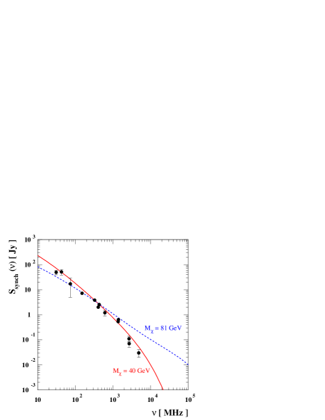
Figure 10: Best fit models for the radio flux density spectrum, in case of a soft spectrum due to a $b\bar{b}$ annihilation final state (solid line, model with $M_{\chi}=40$ GeV) and of a hard spectrum due to a $W^{+}W^{-}$ channel (dashed line, model with $M_{\chi}=81$ GeV); values of all parameters setting the model are given in the text. The datasets is from Thierbach et al. (2003).

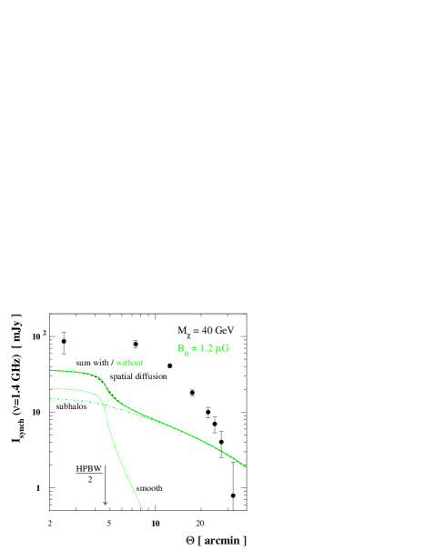
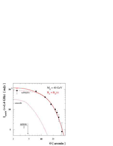
Figure 11: Surface brightness distribution at frequency $\nu=1.4$ GHz, within a beam equal to $9\hbox{$.\mkern-4.0mu^{\prime}$}35$ (HPBW), for the lightest WIMP model displayed in Fig. 10. In the left panel we show the predictions for a model with magnetic field that does not change with radius, and in the limit in which spatial diffusion for electrons and positrons has been neglected (solid line) or included (dashed line). In the right panel we consider a model with magnetic field taking a radial dependence $B(r)=B_{0}\bigg{(}1+{r\over r_{c1}}\bigg{)}^{2}\cdot\bigg{[}1+\bigg{(}{r\over r_{c2}}\bigg{)}^{2}\bigg{]}^{-\beta}$ with $B_{0}=0.55$ $\mu$G  , $\beta=2.7$, $r_{c1}=3^{\prime}$ $r_{c2}=17\hbox{$.\mkern-4.0mu^{\prime}$}5$ in order to reproduce the measured surface brightness. In both cases, the contributions from the smooth dark matter halo component only and from substructures only are also displayed. The dataset is from Deiss et al. (1997).

In Fig. 11 we compare the radio-halo brightness data of Deiss et al. (1997) with the surface brightness distribution $I_{synch}(r)$ predicted at $\nu=1.4$ GHz, within a beam equal to the detector angular resolution (HPBW of $9\hbox{$.\mkern-4.0mu^{\prime}$}35$), for the best fit model with $M_{\chi}=40$ GeV. In the left panel we plot the predicted surface brightness considering the case of a uniform magnetic field equal to $1.2\mu G$, showing explicitly in this case that the assumption we made of neglecting spatial diffusion for electrons and positrons is indeed justified, since the results obtained including or neglecting spatial diffusion essentially coincide. The radial brightness we derive in this case does not match the shape of the radio halo indicated by the data. However, it is easy to derive a phenomenological setup with a magnetic field $B(r)$ varying with radius in which a much better fit can be obtained, while leaving unchanged the total radio flux density $S_{synch.}(\nu)$. We show in the right panel of Fig.11 the predictions for $I_{synch}(r)$ considering a radial dependence of the magnetic field of the form:

$$B(r)=B_{0}\bigg{(}1+{r\over r_{c1}}\bigg{)}^{2}\cdot\bigg{[}1+\bigg{(}{r\over r_{c2}}\bigg{)}^{2}\bigg{]}^{-\beta}\;,$$

which is observationally driven by the available information on the Faraday rotation measures (RM) for Coma (see Fig.16). Such $B(r)$ profile starts at a slightly smaller value in the center of the Coma, rises at a first intermediate scale $r_{c1}$ and then drops rather rapidly at the scale $r_{c2}$. The basic information we provide here is that a radial dependence of the magnetic field like the previous one is required in DM annihilation models to reproduce the radio-halo surface brightness distribution. The specific case displayed is for best-fit values $B_{0}=0.55$ $\mu$G  , $\beta=2.7$, $r_{c1}=3^{\prime}$ $r_{c2}=17\hbox{$.\mkern-4.0mu^{\prime}$}5$, and it provides an excellent fit to the surface brightness radial profile (see Fig.11). In that figure we also plot separately the contributions to the surface brightness due to the smooth DM component (essentially a point-like source in case of this rather poor angular resolution) and the term due to subhalos (which extends instead to larger radii). It is interesting to note that the surface brightness profile can only be fitted by considering the extended sub-halo distribution which renders the DM profile of Coma more extended than the smooth, centrally peaked component. This means that any peaked and smooth DM profile is unable to fit this observable for Coma.
A decrease of $B(r)$ at large radii is expected by general considerations of the structure of radio-halos in clusters and, more specifically, for Coma (see Colafrancesco et al. (2005)) and it is also predicted by numerical simulations (see, e.g., Dolag et al. (2002)): thus it seems quite natural and motivated. At small radii, the mild central dip of $B(r)$ predicted by the previous formula is what is phenomenologically required by the specific DM model we worked out in our paper. Finally, we notice that our specific phenomenological model for the spatial distribution of $B(r)$ is able to reproduce the spatial distribution of Faraday rotation measures (RMs) observed in Coma (see Kim et al. (1990)), as shown in Fig.12.

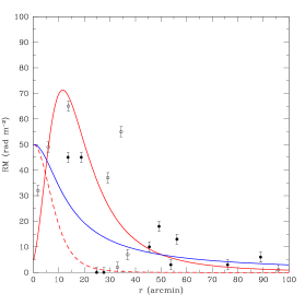
Figure 12: The observed absolute RM of background sources in the Coma field are shown as a function of projected radius $\theta$ in arcmin. The blu curve is the prediction of a model with $B=$ const. The red dashed curve is the prediction of a model with $B(r)$ decreasing monotonically towards large radii and the solid red curve is the prediction of our model that fits the Coma radio-halo surface brightness. Data on positive (filled dots) and negative (empty dots) RMs are from Kim et al. (1990).

It is evident that models in which $B$ is either constant or decreases monotonically towards large radii seem to be difficult to reconcile with the available RM data. The RM data at $\theta\ \raise-2.0pt\hbox{\hbox to0.0pt{\hbox{$\sim$}\hss}\raise 5.0pt\hbox{$<$}\ }20$ arcmin seem to favour, indeed, a model for $B(r)$ with a slight rise at intermediate angular scales followed by a decrease at large scales, like the one we adopt here to fit the radio-halo surface brightness of Coma. In this respect, it seems that our choice for $B(r)$ is, at least, an observationally driven result.

The synchrotron signal produced by the annihilation of DM depends, given the fundamental physics and astrophysics framework, on two relevant quantities: the annihilation rate and the magnetic field. Thus, it is interesting to find the best-fitting region of the $\langle\sigma v\rangle_{0}-B$ plane which is consistent with the available dataset for Coma.

Since the data on the radio flux density spectrum (Thierbach et al. (2003)) is a compilation of measurements performed with different instruments (possibly with different systematics), it is difficult to decide a cut on the $\chi^{2}_{r}$ value which defines an acceptable fit. In Fig. 13 we plot sample isolevel curves for $\chi^{2}_{r}$, spotting the shape of the minima of $\chi^{2}_{r}$ , in the plane $B-\langle\sigma v\rangle_{0}$, for the two sample annihilation channels and a few sample values of the WIMP mass (note that values labeling isolevel curves are sensibly different in the two panels). In Fig. 14 we show the analogous $\chi^{2}_{r}$ isolevels in the WIMP mass – annihilation rate plane, and taking at each point the minimum $\chi^{2}_{r}$ while varying the magnetic field strength between $1\mu G$ and $20\mu G$: the curves converge to a maximal value enforced by the lower limit of $1\mu G$, and the upper value does not enter in defining isolevel curve shapes.

In order to assess whether the outlined radio-data preferred regions are or are not compatible with supersymmetric DM models, we proceed to a random scan of the SUSY parameter space, in the bottom-up approach which we outline below. We relax all universality assumptions, and fully scan the low-energy scale MSSM, imposing phenomenological as well as cosmological constraints on the randomly generated models. We take values of $\tan\beta$, the ratio between the vacuum expectation values of the two Higgs doublets, between 1 and 60. The parameters entering the neutralino mass matrix are generated in the range $1\ {\rm GeV}<m_{1},\ m_{2},\ \mu<1\ {\rm TeV}$, and we define $m_{\rm LSP}\equiv{\rm min}(m_{1},\ m_{2},\ \mu)$. To avoid flavor changing effects in the first two lightest quark generations, we assume that the soft-breaking masses in the first two generations squark sector are degenerate, i.e. we assume $m^{(1)}_{\widetilde{Q},\ \widetilde{U},\ \widetilde{D}}=m^{(2)}_{\widetilde{Q},\ \widetilde{U},\ \widetilde{D}}$. The scalar masses are scanned over the range

$$m_{\rm LSP}\ <\ m^{(1,3)}_{\widetilde{Q}},\ m^{(1,3)}_{\widetilde{U}},\ m^{(1,3)}_{\widetilde{U}},\ m^{(1,2,3)}_{\widetilde{L}},\ m^{(1,2,3)}_{\widetilde{E}},\ m_{A}\ <\ 2.5\ {\rm TeV}$$ (43)

The trilinear couplings are sampled in the range

$$-3\cdot{\rm max}(m^{(i)}_{\widetilde{Q}},\ m^{(i)}_{\widetilde{U}})\ < A_{U}^{(i)} <\ 3\cdot{\rm max}(m^{(i)}_{\widetilde{Q}},\ m^{(i)}_{\widetilde{U}})$$ (44)

$$-3\cdot{\rm max}(m^{(i)}_{\widetilde{Q}},\ m^{(i)}_{\widetilde{D}})\ < A_{D}^{(i)} <\ 3\cdot{\rm max}(m^{(i)}_{\widetilde{Q}},\ m^{(i)}_{\widetilde{D}})$$ (45)

$$-3\cdot{\rm max}(m^{(i)}_{\widetilde{L}},\ m^{(i)}_{\widetilde{E}})\ < A_{E}^{(i)} <\ 3\cdot{\rm max}(m^{(i)}_{\widetilde{L}},\ m^{(i)}_{\widetilde{E}})$$ (46)

Finally, we take the gluino mass in the range $200\ {\rm GeV}<m_{\widetilde{g}}<3\ {\rm TeV}$. The mass ranges for squarks and gluino have been chosen following qualitative criteria (Baer et al. (2003); Battaglia et al. (2003)), so that all viable models generated should be “visible” at the LHC.

We exclude models giving a relic abundance of neutralinos exceeding $\Omega_{\chi}h^{2}>0.13$. Further, we impose the various colliders mass limits on charginos, gluinos, squarks and sleptons, as well as on the Higgs masses. Moreover, we also require the BR($b\rightarrow s\gamma$) and all electroweak precision observables to be consistent with the theoretical and experimental state-of-the-art (Eidelman et al. (2004)).
We classify the models according to the branching ratios of the neutralino pair-annihilations final states, according to the following criteria: we consider a model having a hard spectrum if

$${\rm BR}(W^{+}W^{-})+{\rm BR}(ZZ)>0.8;$$ (47)

a soft spectrum is instead attributed to models satisfying the condition

$$\sum_{i=1}^{6}\left[{\rm BR}(q_{i}\bar{q}_{i})+{\rm BR}(q_{i}\bar{q}_{i}g)\right]+{\rm BR}(gg)>0.8.$$ (48)

We show, in Fig.15 a scatter plots of the viable SUSY configurations, indicating with filled green circles those thermally producing a neutralino relic abundance within the 2-$\sigma$ WMAP range, and with red circles those producing a relic abundance below the WMAP range (whose relic abundance can however be cosmologically enhanced, in the context of quintessential or Brans-Dicke cosmologies, or which can be non-thermally produced, as to make up all of the observed CDM (see Murakami & Wells 2001 and other refs. ). The low $\chi^{2}$ ranges of $\langle\sigma v\rangle_{0}-B$ and $\langle\sigma v\rangle_{0}-M_{\chi}$ values indicated in Figs. 13 and 14 are therefore shown to be actually populated by a number of viable SUSY models.

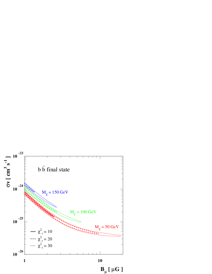
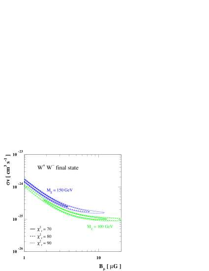
Figure 13: Isolevel curves for reduced $\chi^{2}$ from the fit of the Coma radio flux density spectrum, for a given mass (50 - 100 -150 GeV) and annihilation channel. The halo profile is the best fit N04 profile: $M_{vir}=0.9\,10^{15}M_{\odot}{\ }h^{-1}$ and $c_{vir}=10$, with subhalo setup as in Fig. 6.

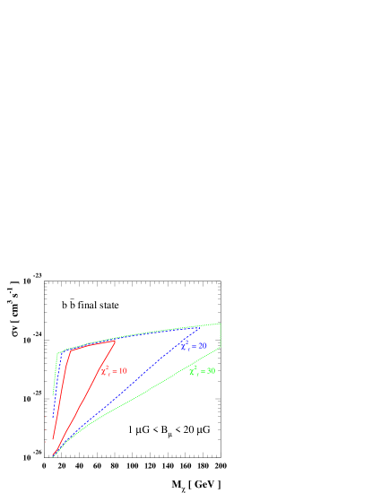
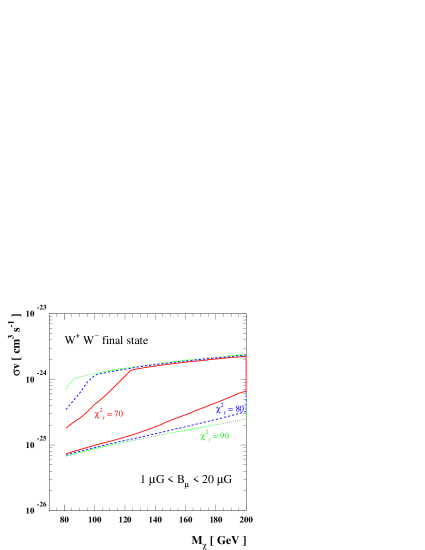
Figure 14: Isolevel curves for minimum reduced $\chi^{2}$ from the fit of the Coma radio flux density spectrum, obtained by varying the magnetic field within $1\mu G\leq B_{\mu}\leq 20\mu G$, for a given annihilation channel. The halo profile is the best fit N04 profile: $M_{vir}=0.9\,10^{15}M_{\odot}{\ }h^{-1}$ and $c_{vir}=10$, with subhalo setup as in Fig. 6.

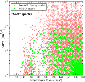
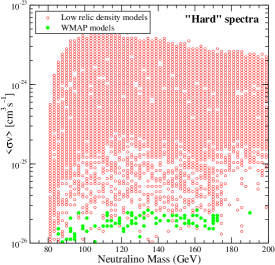
Figure 15: A scatter plot of SUSY models, consistent with all available phenomenological constraints, giving a relic abundance in the 2-$\sigma$ WMAP range (green filled circles) or below it (low, relic density models, red circles), for soft (left panel) and hard (right panel) annihilation spectra.

4.2 From the UV to the gamma-ray band

Inverse Compton (IC) scatterings of relativistic electrons and positrons on target cosmic microwave background (CMB) photons give rise to a spectrum of photons stretching from below the extreme ultra-violet up to the soft gamma-ray band, peaking in the soft X-ray energy band. Let $E=\gamma m_{e}c^{2}$ be the energy of electrons and positrons, $\epsilon$ that of the target photons and $E_{\gamma}$ the energy of the scattered photon. The Inverse Compton power is obtained by folding the differential number density of target photons with the IC scattering cross section:

$$P_{\rm IC}\left(E_{\gamma},E\right)=c\,E_{\gamma}\int d\epsilon\,n(\epsilon)\,\sigma(E_{\gamma},\epsilon,E)$$ (49)

where $n(\epsilon)$ is the black body spectrum of the $2.73K$ CMB photons, while $\sigma(E_{\gamma},\epsilon,E)$ is given by the Klein-Nishina formula:

$$\sigma(E_{\gamma},\epsilon,E)=\frac{3\sigma_{T}}{4\epsilon\gamma^{2}}\,G\left(q,\Gamma_{e}\right)$$ (50)

where $\sigma_{T}$ is the Thomson cross section and

$$G\left(q,\Gamma_{e}\right)\equiv\left[2q\ln q+(1+2q)(1-q)+\frac{\left(\Gamma_{e}q\right)^{2}(1-q)}{2\left(1+\Gamma_{e}q\right)}\right]$$ (51)

with

$$\Gamma_{e}=4\epsilon\gamma/(m_{e}c^{2})\;\;\;\;\;q=E_{\gamma}/\left[\Gamma_{e}\left(\gamma m_{e}c^{2}-E_{\gamma}\right)\right]\;.$$ (52)

Folding the IC power with the spectral distribution of the equilibrium number density of electrons and positrons, we get the local emissivity of IC photons of energy $E_{\gamma}$:

$$j_{\rm IC}\left(E_{\gamma},r\right)=\int dE\,\left(\frac{dn_{e^{-}}}{dE}+\frac{dn_{e^{+}}}{dE}\right)P_{\rm IC}\left(E_{\gamma},E\right)\;$$ (53)

which we use to estimate the integrated flux density spectrum:

$$S_{\rm IC}(E_{\gamma})=\int d^{3}r\,\frac{j_{\rm IC}\left(E_{\gamma},r\right)}{4\pi\,D_{\rm Coma}^{2}}\;.$$ (54)

In Eq. (49) and Eq. (53) the limits of integration over $\epsilon$ and $E_{\gamma}$ are set from the kinematics of the IC scattering which restricts $q$ in the range $1/(4\gamma^{2})\leq q\leq 1$.

The last relevant contribution to the photon emission of Coma due to relativistic electrons and positrons is the process of non-thermal bremsstrahlung, i.e. the emission of gamma-ray photons in the deflection of the charged particles by the electrostatic potential of intra-cluster gas. Labeling with $E=\gamma m_{e}c^{2}$ the energy of electrons and positrons, and with $E_{\gamma}$ the energy of the emitted photons, the local non-thermal bremsstrahlung power is given by:

$$P_{\rm B}\left(E_{\gamma},E,r\right)=c\,E_{\gamma}\sum_{j}n_{j}(r)\,\sigma_{j}(E_{\gamma},E)\;,$$ (55)

with the sum including all species $j$ in the intra-cluster medium, each with number density $n_{j}(r)$ and relative production cross section:

$$\sigma_{j}(E_{\gamma},E)=\frac{3\alpha\sigma_{T}}{8\pi\,E_{\gamma}}\cdot\left[\left(1+(1-E_{\gamma}/E)^{2}\right)\,\phi_{1}-\frac{2}{3}(1-E_{\gamma}/E)\,\phi_{2}\right]$$ (56)

where $\alpha$ is the fine structure constant, $\phi_{1}$ and $\phi_{2}$ two energy dependent scattering functions which depend on the species $j$ (see Longair (1994) for details). The emissivity $j_{\rm B}\left(E_{\gamma},r\right)$ is obtained by folding the power over the equilibrium electron/positron number density, i.e. the analogous of Eq. (53), while the integrated flux density $S_{\rm B}(E_{\gamma})$ is obtained by summing over all relevant sources as in Eq. (54). We apply this scheme to Coma implementing the gas density profile in Eq. (18) by including atomic and molecular hydrogen and correcting for the helium component.

As we have already mentioned, a hard gamma-ray component arises also from prompt emission in WIMP pair annihilations, either in loop suppressed two-body final states giving monochromatic photons, or through the production and prompt decay of neutral pions giving gamma-rays with continuous spectrum. Since photons propagate on straight lines (or actually geodesics), the gamma-ray flux due to prompt emission is just obtained by summing over sources along the line of sight; we will consider terms integrated over volume

$$F_{\gamma}(E_{\gamma})=\int d^{3}r\,\frac{Q_{\gamma}\left(E_{\gamma},r\right)}{4\pi\,D_{\rm Coma}^{2}}\;.$$ (57)

4.3 The multi-frequency SED of Coma

We show in Fig. 16 the multi-frequency SED produced by WIMP annihilation in the two models used to fit the radio halo spectrum of Coma, as shown in Fig. 10.

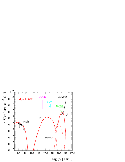
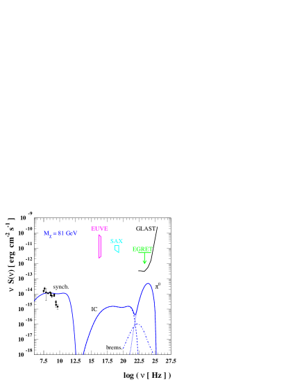
Figure 16: Multi-wavelength spectrum of the two best fit models for the radio flux shown in Fig. 10 (see text for details). The halo profile is the best fit N04 profile: $M_{vir}=0.9\,10^{15}M_{\odot}{\ }h^{-1}$ and $c_{vir}=10$, with subhalo setup as in Fig. 6.

The model with $M_{\chi}=40$ GeV provides the better fit to the radio halo data because the relative equilibrium electron spectrum is steeper and shows also the high-$\nu$ bending which fits the most recent data (Thierbach et al. (2003)). The IC and bremsstrahlung branches of the SED are closely related to the synchrotron branch (since they depend on the same particle population) and their intensity ratio depends basically on the value of the adopted magnetic field. The relatively high value $B=1.2$ $\mu$G  indicated by the best fit to the radio data implies a rather low intensity of the IC and bremsstrahlung emission, well below the EUV and hard X-ray data for Coma. Nonetheless, the gamma-ray emission due to $\pi^{0}\to\gamma\gamma$ decay predicted by this model could be detectable with the GLAST-LAT detector, even though it is well below the EGRET upper limit.

The detectability of the multi-frequency SED worsens in the model with $M_{\chi}=81$ GeV, where the flatness of the equilibrium electron spectrum cannot provide an acceptable fit to the radio data. Moreover, the adopted value of the magnetic field $B=8$ $\mu$G  implies a very low intensity of the IC, bremsstrahlung and $\pi^{0}\to\gamma\gamma$ emission, which should be not detectable by the next generation HXR and gamma-ray experiments.

The energetic electrons and positrons produced by WIMP annihilation have other interesting astrophysical effects among which we will discuss specifically in the following the Sunyaev-Zel’dovich (hereafter SZ) effect produced by DM annihilation and the heating of the intracluster gas produced by Coulomb collisions.

4.4 SZ effect

The energetic electrons and positrons produced by WIMP annihilation interact with the CMB photons and up-scatter them to higher frequencies producing a peculiar SZ effect (as originally realized by Colafrancesco (2004)) with specific spectral and spatial features.

The generalized expression for the SZ effect which is valid in the Thomson limit for a generic electron population in the relativistic limit and includes also the effects of multiple scatterings and the combination with other electron population in the cluster atmospheres has been derived by Colafrancesco et al. (2003). This approach is the one that should be properly used to calculate the specific SZ_DM effect induced by the secondary electrons produced by WIMP annihilation. Here we do not repeat the description of the analytical technique and we refer to the general analysis described in Colafrancesco et al. (2003). According to these results, the DM induced spectral distortion is

$$\Delta I_{\rm DM}(x)=2\frac{(k_{\rm B}T_{0})^{3}}{(hc)^{2}}y_{\rm DM}\leavevmode\nobreak\ \tilde{g}(x)\leavevmode\nobreak\ ,$$ (58)

where $T_{0}$ is the CMB temperature and the Comptonization parameter $y_{\rm DM}$ is given by

$$y_{\rm DM}=\frac{\sigma_{T}}{m_{\rm e}c^{2}}\int P_{\rm DM}d\ell\leavevmode\nobreak\ ,$$ (59)

in terms of the pressure $P_{\rm DM}$ contributed by the secondary electrons produced by neutralino annihilation. The quantity $y_{\rm DM}\propto\langle\sigma v\rangle_{0}n^{2}_{\chi}$ and scales as $\propto\langle\sigma v\rangle_{o}M^{-2}_{\chi}$, providing an increasing pressure $P_{\rm DM}$ and optical depth $\tau_{\rm DM}=\sigma_{T}\int d\ell n_{\rm e}$ for decreasing values of the neutralino mass $M_{\chi}$. The function $\tilde{g}(x)$, with $x\equiv h\nu/k_{\rm B}T_{0}$, can be written as

$$\tilde{g}(x)=\frac{m_{\rm e}c^{2}}{\langle k_{\rm B}T_{\rm e}\rangle}\left\{\frac{1}{\tau}\left[\int_{-\infty}^{+\infty}i_{0}(xe^{-s})P(s)ds-i_{0}(x)\right]\right\}$$ (60)

in terms of the photon redistribution function $P(s)$ and of $i_{0}(x)=2(k_{\rm B}T_{0})^{3}/(hc)^{2}\cdot x^{3}/(e^{x}-1)$, where we defined the quantity

$$\langle k_{\rm B}T_{\rm e}\rangle\equiv\frac{\sigma_{\rm T}}{\tau}\int Pd\ell=\frac{\int Pd\ell}{\int n_{\rm e}d\ell}=\int_{0}^{\infty}dpf_{\rm e}(p)\frac{1}{3}pv(p)m_{\rm e}c$$ (61)

(see Colafrancesco et al. (2003); Colafrancesco (2004)), which is the analogous of the average temperature for a thermal population (for a thermal electron distribution $\langle k_{\rm B}T_{\rm e}\rangle=k_{\rm B}T_{\rm e}$ obtains, in fact). The photon redistribution function $P(s)=\int dpf_{\rm e}(p)P_{\rm s}(s;p)$ with $s=\ln(\nu^{\prime}/\nu)$, in terms of the CMB photon frequency increase factor $\nu^{\prime}/\nu={4\over 3}\gamma^{2}-{1\over 3}$, depends on the electron momentum ($p$) distribution, $f_{\rm e}(p)$, produced by WIMP annihilation.

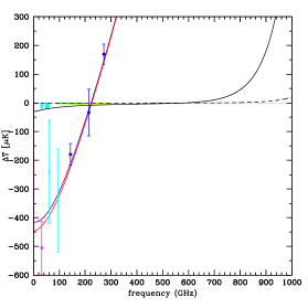
Figure 17: The SZ effect produced by the $b\bar{b}$ model with $M_{\chi}=40$ GeV (black solid curve) and by the $W^{+}W^{-}$ model with $M_{\chi}=81$ GeV (black dashed curve) in Coma are shown in comparison with the thermal SZ effect of Coma (blue curve). The red curves represent the overall SZ effect. Notice that the DM-induced SZ effect has a very different spectral behavior with respect to the thermal SZ effect. SZ data are from OVRO (magenta), WMAP (cyan) and MITO (blue). The sensitivity of PLANCK (18 months, 1 $\sigma$) is shown for the LFI detector at 31.5 and 53 GHz channels (cyan shaded regions) and for the HFI detector 143 and 217 GHZ channels (green and yellow shaded areas, respectively).

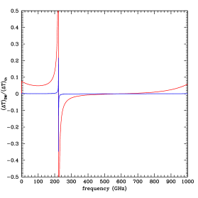
Figure 18: The ratio between the DM-induced and the thermal SZ effect in Coma is shown for the model with $M_{\chi}=40$ GeV (red curve) and for the model with $M_{\chi}=81$ GeV (blue curve). The model with $M_{\chi}=40$ GeV produces an SZ effect which could be detected with the next coming microwave experiments.

We show in Fig.17 the frequency dependence of the CMB temperature change,

$${\Delta T\over T_{0}}={(e^{x}-1)^{2}\over x^{4}e^{x}}{\Delta I\over I_{0}}\,,$$ (62)

as produced by the DM-induced SZ effect in the two best fit WIMP models here considered, compared to the temperature change due to the thermal SZ effect produced by the intracluster gas. The most recent analysis of the thermal SZ effect in Coma (DePetris et al. (2003)) provides an estimate of the optical depth of the thermal intracluster gas $\tau_{th}=4.9\cdot 10^{-3}$ which best fits the data. The model with $M_{\chi}=40$ GeV provides a detectable SZ_DM effect which has a quite different spectral shape with respect to the thermal SZ effect: it yields a temperature decrement at all the microwave frequencies, $\ \raise-2.0pt\hbox{\hbox to0.0pt{\hbox{$\sim$}\hss}\raise 5.0pt\hbox{$<$}\ }600$ GHz, where the thermal SZ effect is observed and produces a temperature increase only at very high frequencies $>600$ GHz. This behavior is produced by the large frequency shift of CMB photons induced by the relativistic secondary electrons generated by the WIMP annihilation. As a consequence, the zero of the SZ_DM effect is effectively removed from the microwave range and shifted to a quite high frequency $\sim 600$ GHz with respect to the zero of the thermal SZ effect, a result which allows one, in principle, to estimate directly the pressure of the electron populations and hence to derive constraints on the WIMP model (see Colafrancesco (2004)).

The presence of a substantial SZ_DM effect is likely to dominate the overall SZ signal at frequencies $x\ \raise-2.0pt\hbox{\hbox to0.0pt{\hbox{$\sim$}\hss}\raise 5.0pt\hbox{$>$}\ }3.8-4.5$ providing a negative total SZ effect. It is, however, necessary to stress that in such frequency range there are other possible contributions to the SZ effect, like the kinematic effect and the non-thermal effect which could provide additional biases (see, e.g., Colafrancesco et al. (2003)). Nonetheless, the peculiar spectral shape of the $SZ_{\rm DM}$ effect is quite different from that of the kinematic SZ effect and of the thermal SZ effect and this result allows us to disentangle it from the overall SZ signal. An appropriate multi-frequency analysis of the overall SZ effect based on observations performed on a wide spectral range (from the radio to the sub-mm region) is required to separate the various SZ contributions and to provide an estimate of the DM induced SZ effect. In fact, simultaneous SZ observations at low frequencies $\sim 30$ GHz (where there is the largest temperature decrement due to SZ_DM), at $\sim 150$ GHz (where the SZ_DM deepens the minimum in $\Delta I/I$ with respect to the dominant thermal SZ effect), at $\sim 220$ GHz (where the SZ_DM dominates the overall SZ effect and produces a negative signal instead of the expected $\approx$ null signal) and at $\ \raise-2.0pt\hbox{\hbox to0.0pt{\hbox{$\sim$}\hss}\raise 5.0pt\hbox{$>$}\ }250$ GHz (where the still negative SZ_DM decreases the overall SZ effect with respect to the dominant thermal SZ effect) coupled with X-ray observations which determine the gas distribution within the cluster (and hence the associated dominant thermal SZ effect) can separate the SZ_DM from the overall SZ signal, and consequently, set constraints on the WIMP model.

The WIMP model with $M_{\chi}=40$ GeV produces a temperature decrement which is of the order of $\sim$ 40 to 15 $\mu$K for SZ observations in the frequency range $\sim$ 30 to 150 GHz (see Fig.17). These signals are still within the actual uncertainties of the available SZ data for Coma and are below the current SZ sensitivity of WMAP (see, e.g., Bennet et al. (2003) and the results of the analysis of the WMAP SZ signals from a sample of nearby clusters performed by Lieu et al. (2005)). Nonetheless, such SZ signals could be detectable with higher sensitivity experiments. The high sensitivity planned for the future SZ experiments can provide much stringent limits to the additional SZ effect induced by DM annihilation. In this context, the next coming sensitive bolometer arrays (e.g., APEX), interferometric arrays (e.g., ALMA) and the PLANCK-HFI experiment, or the planned OLIMPO balloon-borne experiment, have enough sensitivity to probe the contributions of various SZ effects in the frequency range $\nu\approx 30-250$ GHz, provided that accurate cross-calibration at different frequencies can be obtained. The illustrative comparison (see Fig.17) between the model predictions and the sensitivity of the PLANCK LFI and HFI detectors at the optimal observing frequencies ($\nu=31.5$ and $53$ GHz for the LFI detector and $\nu=143$ and $217$ GHz for the HFI detector) show that the study of the SZ effect produced by DM annihilation is actually feasible with the next generation SZ experiments. We show in Fig.18 the expected ratio between the DM-induced SZ effect and the thermal SZ effect for the two WIMP models here considered. It is evident that while the model with $M_{\chi}=40$ GeV provides a detectable signal which is a sensitive fraction of the thermal SZ effect at $\nu<250$ GHz, the SZ signal provided by the model with $M_{\chi}=81$ GeV is by far too small to be detectable at any frequency.
The spectral properties shown by the SZ_DM for neutralinos depends on the specific neutralino model as we have shown in Fig.17: in fact, the SZ effect is visible for a neutralino with $M_{\chi}=40$ GeV and not visible for a neutralino with $M_{\chi}=81$ GeV. Thus the detailed features of the SZ effect from DM annihilation depends strongly on the mass and composition of the DM particle, and - in turn - on the equilibrium spectrum of the secondary electrons. Each specific DM model predicts its own spectrum of secondary electrons and this influences the relative SZ effect. Models of DM which provide similar electron spectra will provide similar SZ effects.

4.5 Heating of the intracluster gas

Low energy secondary electrons produced by WIMP annihilation might heat the intracluster gas by Coulomb collisions since the Coulomb loss term dominates the energy losses at $E\ \raise-2.0pt\hbox{\hbox to0.0pt{\hbox{$\sim$}\hss}\raise 5.0pt\hbox{$<$}\ }200$ MeV (see Fig. 26). The specific heating rate is given by

$${dE\over dtdV}=\int dE{dn_{e}\over dE}\cdot\bigg{(}{dE\over dt}\bigg{)}_{Coul}$$ (63)

where ${dn_{e}\over dE}$ is the equilibrium electron spectrum derived in Sect. A and the Coulomb loss rate is $(dE/dt)_{Coul}=b_{Coul}^{0}n\left(1+\log(\gamma/n)/75\right)$ where $n$ is the mean number density of thermal electrons in $\rm{cm}^{-3}$ (see Eq. 18, the average over space gives about $n\simeq 1.3\;10^{-3}$), $\gamma\equiv E/m_{e}$ and $b_{Coul}^{0}\simeq 6.13\cdot 10^{-16}\;\rm{GeV}\,\rm{s}^{-1}$.

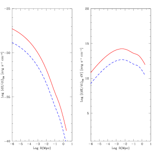
Figure 19: Left: the specific heating rate is plotted against the radial distance from the center of Coma. Right: the specific heating rate multiplied by the volume element is plotted against the radial distance from the center of Coma.

Fig.19 shows the specific heating rate of Coma as produced in the two WIMP models explored here. The non-singular N04 halo model adopted in our analysis does not provide a high specific heating rate at the cluster center, and thus one might expect an overall heating rate for Coma which is of order of $\sim 10^{38}$ erg/s ($\sim 10^{36}$ erg/s) for the WIMP model with $M_{\chi}=40$ GeV ($M_{\chi}=81$ GeV). We also notice that the region that mostly contributes to the overall heating of Coma is not located at the center of the cluster. This is again a consequence of the non-singular N04 DM profile which has been adopted. The diffusion of electrons in the innermost regions of Coma acts in the same direction and moves the maximum of the curves shown in the right panel of Fig.19 towards the outskirts of Coma, even in the case of a halo density profile which is steeper than the adopted one.
This implies, in conclusion, that WIMP annihilation cannot provide most of the heating of Coma, even in its innermost regions. Such a conclusion seems quite general and implies that non-singular DM halo models are not able to provide large quantities of heating at the center of galaxy clusters so to quench efficiently the cooling of the intracluster gas (with powers of $\sim 10^{43-45}$ erg/s). Only very steep halo profiles (even steeper than the Moore profile) and with the possible adiabatic growth of a central matter concentration (e.g., a central BH) could provide sufficient power to quench locally (i.e. in the innermost regions) the intracluster gas cooling (see, e.g., Totani (2004)). However, we stress that the spatial diffusion of the secondary electrons in the innermost regions of galaxy clusters should flatten the specific heating rate in the vicinity of the DM spike and thus decrease substantially the heating efficiency by Coulomb collisions. In conclusion, we believe that the possibility to solve the cooling flow problem of galaxy clusters by WIMP annihilation is still an open problem.

5 Discussion

WIMP annihilation in galaxy cluster is an efficient mechanism to produce relativistic electrons and high-energy particles which are able, in turn, to produce a wide SED extended over more than 18 orders of magnitude in frequency, from radio to gamma-rays. We discuss here the predictions of two specific models which embrace a vast range of possibilities.

The $b{\bar{b}}$ model with $M_{\chi}=40$ GeV and annihilation cross section $\langle\sigma v\rangle_{0}=4.7\cdot 10^{-25}cm^{3}s^{-1}$ provides a reasonable fit to the radio data (both the total spectrum and the surface brightness radial distribution) with a magnetic field whose mean value is $B\approx 1.2\mu$G. We remind here that the quite high value of $\langle\sigma v\rangle_{0}$ is well inside the range of neutralino masses and annihilation cross-sections provided by the most general supersymmetric DM setup (see our discussion in Sect.3.2). Table 3 provides an illustrative scheme of the radiation mechanisms, of the particle energies and of the fluxes predicted by this best-fit WIMP model for a wide range of the physical conditions in the cluster atmosphere.

	$\nu$	$\nu F(\nu)$	$E_{particle}$	Mechanism
	[GHz]	[$ergs^{-1}cm^{-2}$]	[GeV]
Radio	$1.4$	$6.4\cdot 10^{-15}$	$17.3\cdot B^{-1/2}_{\mu}$	$e^{\pm}$ Synchrotron
Optical	$(7.25-14.5)\cdot 10^{5}$	$1.7\cdot 10^{-15}$	$(1.9-2.7)\cdot 10^{-2}$	$e^{\pm}$ ICS
EUV	$(0.31-0.43)\cdot 10^{8}$	$5.2\cdot 10^{-14}$	$0.13-0.15$	$e^{\pm}$ ICS
HXR	$(4.83-19.3)\cdot 10^{9}$	$1.0\cdot 10^{-13}$	$1.56-3.13$	$e^{\pm}$ ICS
		$1.2\cdot 10^{-17}$	$(4-16)\cdot 10^{-5}$	$e^{\pm}$ Bremsstrahlung
$\gamma$-ray	$2.42\cdot 10^{14}$	$6.6\cdot 10^{-13}$	$2$	$\pi^{0}\to\gamma\gamma$ decay
		$2.2\cdot 10^{-15}$	$2$	$e^{\pm}$ Bremsstrahlung

Table 3: Predicted flux in various frequency ranges for a neutralino $b{\bar{b}}$ model with $M_{\chi}=40$ GeV and $\langle\sigma v\rangle=10^{-26}$ cm³/s. The value of the magnetic field is $B_{\mu}=1.2\,\mu$G. $E_{particle}$ refers to the approximate energy for $e^{\pm}$ or $\gamma$ sourcing the corresponding flux in the monochromatic limit.

For the best-fit values of $M_{\chi}=40$ GeV and $\langle\sigma v\rangle_{0}=4.7\cdot 10^{-25}cm^{3}s^{-1}$ this model yields EUV and HXR fluxes which are more than one order of magnitude fainter than the Coma data. The gamma-ray flux produced by this model is dominated by the continuum $\pi^{0}\to\gamma\gamma$ component and it is a factor $\sim 5$ lower than the EGRET upper limit of Coma at its peak frequency (see Fig. 16, left panel). Such gamma-ray flux could be, nonetheless, detectable by the GLAST–LAT detector (we will discuss more specifically the detectability of the gamma-ray WIMP annihilation signals from galaxy clusters in a dedicated, forthcoming paper (Colafrancesco, Profumo & Ullio 2006b). The rather low neutralino mass $M_{\chi}=40$ GeV of this model makes it rather difficult to be testable by Cherenkov gamma-ray detectors operating at higher threshold energies.

Increasing the neutralino mass does not provide a good fit of the radio-halo spectrum (see Fig. 16, right panel) and yields, in addition, extremely faint EUV, HXR and gamma-ray fluxes, which turn out to be undetectable even by GLAST and/or by the next coming high-energy experiments.

It is possible to recover the EUV and HXR data on Coma with a IC flux by secondary electrons by increasing the annihilation cross-sections by a factor $\sim 10^{2}$ (i.e., up to values $\langle\sigma v\rangle_{0}\approx 7\cdot 10^{-23}cm^{3}s^{-1}$) in the best-fit $b{\bar{b}}$ soft WIMP model (at fixed $M_{\chi}=40$ GeV). However, in such a case both the radio-halo flux and the hard gamma-ray flux at $\sim 1$ GeV as produced by $\pi^{0}$ decay should increase by the same factor leading to a problematic picture: in fact, while the radio-halo data would imply lower values of the magnetic field $B\sim 0.1$ $\mu$G  which might still be allowed by the data, the $\pi^{0}\to\gamma\gamma$ gamma-ray flux at $E>100$ MeV should exceed the EGRET limit on Coma. This option is therefore excluded by the available data.
Alternatively, it would be possible to fit the EUV and HXR spectra of Coma with the adopted value of $\langle\sigma v\rangle_{0}\approx 7\cdot 10^{-23}cm^{3}s^{-1}$ for the $b{\bar{b}}$ model with $M_{\chi}=40$ GeV, in the case we sensibly lower the mean magnetic field. Values of the average magnetic field $\ \raise-2.0pt\hbox{\hbox to0.0pt{\hbox{$\sim$}\hss}\raise 5.0pt\hbox{$<$}\ }0.2\mu$G are required to fit the HXR flux of Coma under the constraint to fit at the same time the radio-halo spectrum (see Fig.20, left panel), consistently with the general description of the ratio between the synchrotron and IC emission powers in Coma (see, e.g., Colafrancesco et al. (2005), Reimer et al. (2004)). Magnetic fields as low as $\sim 0.15\mu$G can fit both the HXR and the EUV fluxes of Coma. However, also in this case the $\pi^{0}\to\gamma\gamma$ gamma-ray flux predicted by the same model at $E>100$ MeV exceeds the EGRET limit on Coma, rendering untenable this alternative. Actually, the EGRET upper limit on Coma set a strong constraint on the combination of values $B$ and $\langle\sigma v\rangle_{0}$ (see Fig.20, right panel) so that magnetic field larger than $\ \raise-2.0pt\hbox{\hbox to0.0pt{\hbox{$\sim$}\hss}\raise 5.0pt\hbox{$>$}\ }0.3$ $\mu$G  are required for the parameter setup of the $b{\bar{b}}$ model with $M_{\chi}=40$ GeV. Fig.20 shows the upper limits on the value of $\langle\sigma v\rangle$ as a function of the assumed value of the mean magnetic field of Coma. According to these results, it is impossible to fit all the available data on Coma for a consistent choice of the DM model and of the cluster magnetic field. The EUV and HXR data in particular require extreme conditions, i.e. low values of the magnetic field and/or high values of the annihilation cross section, which violate the EGRET gamma-ray limit. Thus, realistic DM models that are consistent with the radio and gamma-ray constraints predict IC emission which falls short of fitting the EUV and HXR data of Coma.

An appealing property of the WIMP model worked out here is that it can reproduce both the spatial distribution of the radio-halo surface brightness of Coma and, in principle, also the spatial profile of the EUV emission (see, e.g., Bowyer et al. (2004)) which seems more concentrated than the radio-halo surface brightness. As for the radio-halo surface brightness profile, it seems necessary for this WIMP model - due to the shape of the DM halo profile - to invoke a radial distribution of the magnetic field with a mild decrease towards the Coma center to counterbalance the centrally peaked DM profile, and with an exponential cutoff at large radii to counterbalance the effect of the subhalo distribution. We notice here that such a specific $B(r)$ spatial distribution is - interestingly enough - able to reproduce the radial distribution of the RMs in Coma (see Sect.5.1). While the (Synchrotron) radio surface brightness depends strongly on the magnetic field radial profile, the (ICS) EUV radial profile only depends on the DM halo profile and on the secondary electron properties and is, hence, more concentrated (see Fig. 10 for an example). Thus, the radial distribution of the EUV emission could be reasonably reproduced by the WIMP model which best fits the radio data but with a very low value of the magnetic field of order of $\ \raise-2.0pt\hbox{\hbox to0.0pt{\hbox{$\sim$}\hss}\raise 5.0pt\hbox{$<$}\ }0.15$ $\mu$G. We already noticed, however, that models with values of the average magnetic field in Coma which are $\ \raise-2.0pt\hbox{\hbox to0.0pt{\hbox{$\sim$}\hss}\raise 5.0pt\hbox{$<$}\ }0.3\mu$G produce a gamma-ray flux which exceeds the EGRET upper limit of Coma (see Fig. 20), rendering these models untenable.

We summarize all the constraints on the neutralino models set by the magnetic field and by the annihilation cross-section in Figs. 20 and 21. The available data set constraints on the WIMP annihilation rate. Figs.22 and 23 show the upper limits on $\langle\sigma v\rangle_{0}$ as a function of the assumed value for the mean magnetic field in Coma. The EGRET limit proves to be the more constraining at the moment with respect to the HXR and EUV data. These limits are able to test directly the annihilation rate since they are independent of the magnetic field value. Nonetheless, the combination of the gamma-ray and/or HXR constraints with the radio constraints will be able to determine the full setup of the relevant quantities whose combination is able to fit the overall Coma SED. In this context, it is clear that the possible GLAST observations of Coma, combined with the radio data, will increase by far the constraints in the $\langle\sigma v\rangle_{0}-B$ plane.

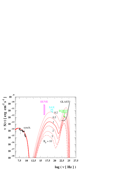
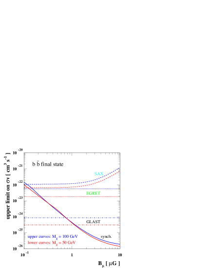
Figure 20: Scaling of the multi-wavelength spectrum and of relative bounds on the particle physics model with the assumed value for the mean magnetic field in Coma. Left panel: we have chosen a few sample values for the magnetic field and varied freely pair annihilation cross section and WIMP mass to minimize the $\chi^{2}$ for the fit of radio data (a $b\,\bar{b}$ final state is assumed); the decrease in the magnetic field must be compensated by going to larger $M_{\chi}$ and $\langle\sigma v\rangle_{0}$, with a net increase in $\langle\sigma v\rangle_{0}/M_{\chi}^{2}$, as it can be seen from the increase in the $\pi^{0}$ component. The increase in the IC component is, at large values for the magnetic field, significantly more rapid, since for large values of the magnetic field synchrotron losses are the main energy loss mechanism for electrons and positrons and tend to decrease the number density for the equilibrium population. Right panel: upper limit on $\langle\sigma v\rangle_{0}$ as a function of the assumed value for the mean magnetic field in Coma; at each wavelength the limit is derived assuming that the predicted flux should be lower than the upper limit from each individual data point (slight overestimate of the limit from radio data, but we do not need to decide the cut on the reduced $\chi^{2}$ marking the overshooting of the radio flux). Two sample values of $M_{\chi}$ are assumed. The lines marked GLAST refer to the GLAST projected sensitivity assuming no other $\gamma$-ray component is present. In both panels the halo profile is the best fit N04 profile: $M_{vir}=0.9\,10^{15}M_{\odot}{\ }h^{-1}$ and $c_{vir}=10$, with subhalo setup as in Fig. 6.

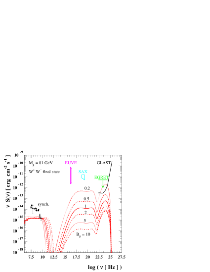
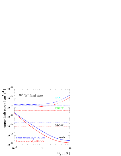
Figure 21: The analogous of Fig. 20, but now for the $W^{+}W^{-}$ final state and fixing the WIMP mass to 81 GeV. In the left panel, for each value of the magnetic field, the value of $\langle\sigma v\rangle_{0}$ is obtained by normalizing the radio flux at the value of the flux at the highest frequency point in the available dataset. Note again that on fair fit of the full radio dataset can be derived for this hard channel.

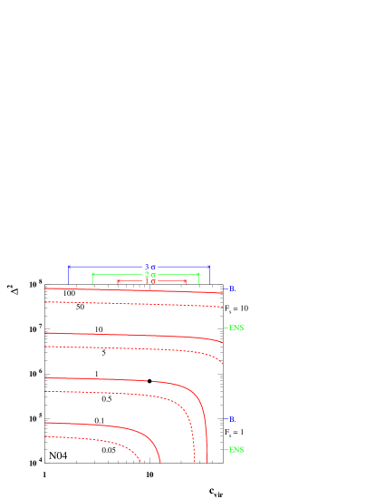
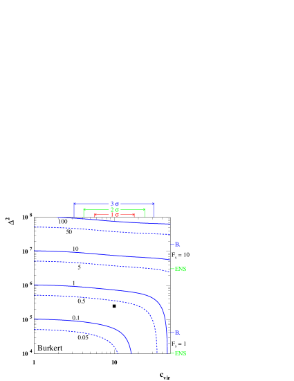
Figure 22: Scaling of fluxes with the assumptions on the halo model for Coma. In the plane $c_{vir}$ – $\Delta^{2}$ we plot isolevel curves for fluxes normalized to the corresponding values within the setup as for the N04 profile in Fig. 6, marked with a dot in the left panel, i.e. the halo model we have assumed so far as reference model; the model marked with square in the right panel corresponds to the Burkert profile selected in Fig. 6. For all examples displayed we have fixed $M_{vir}=0.9\,10^{15}M_{\odot}{\ }h^{-1}$ and a 50% mass in substructures. The left panel refers to N04 profiles, the right panel to Burkert profiles; reference values for $c_{vir}$ and $\Delta^{2}$, as obtained by fitting the corresponding halo profiles and from our discussion on the substructure role, are marked on the axis. Switching to one of the halo models displayed here is equivalent to shifting all values of $\langle\sigma v\rangle_{0}$ plotted in figures to $\langle\sigma v\rangle_{0}$ divided by the scaling value shown here.

The results of our analysis also depend on the assumed DM halo density profile. Fig. 22 shows the scaling of fluxes with the assumptions on the halo model for Coma. We compare here, for the sake of illustration, the scalings of the N04 and of the Burkert model. Switching to one of the halo models displayed here is equivalent to shifting all values of $\langle\sigma v\rangle_{0}$ plotted in the figures to $\langle\sigma v\rangle_{0}$ divided by the scaling value shown here. This analysis allows us to compare correctly the results of the multi-frequency analysis we have presented in this paper in terms of substructure enhancement and halo density profile.

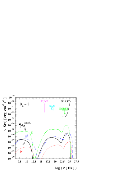
Figure 23: Multi-wavelength spectra for the four benchmark models described in the text. The prediction is shown for the best fit N04 profile, and our reference choice for subhalo parameters, and for a mean magnetic field equal to $2\mu G$.

Table 4 also shows the typical values for the annihilation cross-section $\langle\sigma v\rangle_{0}$ and the relative signals expected at different frequencies for the Coma best-fit model ($b{\bar{b}}$ neutralino model with $M_{\chi}=40$ GeV and $B=1$ $\mu$G) that we explored in this paper.

	Cuspy profile	Cored profile
Coma cluster	$\langle\sigma v\rangle_{0}$ (${\rm cm^{3}}\ {\rm s^{-1}}$)	$\langle\sigma v\rangle_{0}$ (${\rm cm^{3}}\ {\rm s^{-1}}$)
Radio	$5\cdot 10^{-25}$	$5\cdot 10^{-24}$
EUV	$3\cdot 10^{-23}$	$3\cdot 10^{-22}$
HXR	$2.5\cdot 10^{-23}$	$2.5\cdot 10^{-22}$
$\gamma$-ray (EGRET limit)	$1.3\cdot 10^{-23}$	$1.3\cdot 10^{-22}$
$\gamma$-ray (GLAST limit)	$7.5\cdot 10^{-25}$	$7.5\cdot 10^{-24}$
Milky Way	$\langle\sigma v\rangle_{0}$ (${\rm cm^{3}}\ {\rm s^{-1}}$)	$\langle\sigma v\rangle_{0}$ (${\rm cm^{3}}\ {\rm s^{-1}}$)
Positrons	$\sim 10^{-26}$	$\sim 10^{-25}$
Antiprotons	$\sim 10^{-27}$	$\sim 10^{-26}$
Antideuterons	$\sim 10^{-27}$	$\sim 10^{-26}$
$\gamma$-ray (GLAST limit)	$\sim 10^{-28}$	$\sim 10^{-23}$

Table 4: Order-of-magnitude estimates of the values of the cross-section, $\langle\sigma v\rangle_{0}$, in units of ${\rm cm^{3}}\ {\rm s^{-1}}$, needed to reproduce the detected non-thermal emission features in Coma and to produce sizable signals for future indirect dark matter search experiments in the Milky Way.

Large neutralino pair annihilation cross section will, in general, produce sizable signals also for other indirect detection techniques, including antimatter searches and gamma rays from the center of the Milky Way. Antimatter and gamma-ray fluxes also largely depend on the Milky Way dark-matter halo and on the specific neutralino model (e.g. through the antimatter yield per neutralino annihilation). Existing analysis (Baer and Profumo (2005); Profumo and Ullio (2004); Baer et al. 2005a ; Profumo (2005)) make it possible to draw some qualitative estimates of the cross-section, $\langle\sigma v\rangle_{0}$, required to produce sensible signals at future DM search experiments. We provide in Table 4 order-of-magnitude estimates for the value of $\langle\sigma v\rangle_{0}$ expected to give observable signals in space-based antimatter (AMS-02, Pamela, GAPS) and gamma-ray search experiments (GLAST), for two extreme choices of the galactic dark-matter halo: a cuspy profile (such as the N04 profile) and a cored profile (such as the Burkert profile). Different search techniques, such as direct detection, or neutrino flux detection from the core of the Sun induced by the annihilation of captured neutralinos, critically depend upon the scattering cross section of neutralinos off nucleons, and the resulting detection rates are therefore unrelated, in general, to the pair annihilation process discussed here.

We show in Fig. 23 the overall SED of Coma as expected from the four benchmark models described in the Sect.3.2. The predictions are shown for the best fit N04 profile and for our reference choice for subhalo parameters, and for a mean magnetic field of $2\mu G$. None of these benchmark model may provide a reasonable fit to the radio data. Notice, in addition, the quite dim multi-frequency SED predicted for Coma in these benchmark models. The largest fluxes are, not surprisingly, obtained for the model lying in the focus point region ($E^{\prime}$). In that case, neutralinos mostly annihilate into gauge bosons, as can be inferred from the spectral shape, which closely resembles that in Fig. 21. We therefore conclude that the expectation of astrophysical signatures from neutralino DM annihilations in the Coma cluster (with natural assumptions on the dark halo profile, substructures and magnetic field of Coma) is not promising in the context of the commonly discussed minimal supergravity scenario.

It would be interesting to compare the predictions of the WIMP annihilation for Coma with the implication of the presence of another population of cosmic rays of different origin like that, often invoked, produced by acceleration processes in the atmosphere of Coma. Acceleration scenarios usually produce power-law spectra for the electrons which are primarily accelerated by shocks or turbulence and are, hence remarkably different from the source spectra produced by neutralino acceleration. Specifically, acceleration models do not exhibit a cut-off at the neutralino mass and do not produce the peculiar peaked $\pi^{0}$ gamma-ray emission which remains a distinctive feature of neutralino DM models. A continuum $\pi^{0}$ gamma-ray emission can be produced in secondary models where the electrons are produced by proton-proton collision in the cluster atmosphere. But even in this case the gamma-ray spectrum is likely to be resembled by a power-law shape which keeps memory of the original acceleration events for the hadrons. Thus, it will be possible to separate DM annihilation models from acceleration models based on multi-frequency observations of the hadronic and leptonic components of the cluster SED.

Finally, It should be noticed that the same problem with the consistent fitting of both the synchrotron and IC components to the radio and EUV/HXR data of Coma still remains in both DM and acceleration models, pointing to the fact that these spectral features, if real, have probably different physical origin.

6 Summary and conclusions

WIMP annihilations in galaxy cluster inevitably produce high-energy secondary particles which are able, in turn, to produce a wide SED extended over more than 18 orders of magnitude in frequency, from radio to gamma-rays.

A consistent analysis of the DM distribution and of its annihilation in the Coma cluster shows that WIMP annihilation is able to reproduce both the spectral and the spatial features of the Coma radio halo under reasonable assumptions for the structure of the intracluster magnetic field. The mild decrease of the magnetic field towards the Coma center, which reproduces the radial trend of the observed RM distribution in Coma, could be better tested with a larger dataset of Faraday rotation measures of background radio sources obtainable with the next generation sensitive radio telescopes (LOFAR, SKA), and with the help of numerical MHD simulations. Radio data are the main constraint, so far, to WIMP models.

The ICS emission produced by the same secondary electrons is able, in principle, to reproduce both the spectrum and the spatial distribution of the EUV emission observed in Coma, provided that a quite small average magnetic field $B\sim 0.15$ $\mu$G  is assumed. Such low value of the B field is also able to make the radio data and the hard X-ray data of Coma consistent within a Synchrotron/IC model for their origins. However, such low magnetic field values in Coma produce an unacceptably large gamma-ray flux, which exceeds the EGRET upper limit. The gamma-ray constraints are thus the most stringent ones for the analysis of the astrophysical features of DM annihilations.

In conclusion, the viable models of WIMP annihilation which are consistent with the available data for Coma yield a nice fit to the radio data but produce relatively low intensity emission at EUV, X-ray and gamma-ray frequencies. The hadronic gamma-ray emission could be, nonetheless, detected by the GLAST-LAT detector. These models also produce negligible heating rates for the kind of non-singular halo profile we worked out in this paper. It is interesting that the best-fit ($b\bar{b}$) WIMP model with $M_{\chi}=40$ GeV predicts a detectable SZ effect (with a peculiar spectrum very different from that of the thermal SZ effect) at the level of $\sim$ 40 to 10 $\mu$K in the frequency range $\sim 10-200$ GHz, which could be observable with the next generation high-sensitivity bolometric arrays, space and balloon-borne microwave experiments, like PLANCK, OLIMPO, APEX, ALMA.

The observational ”panorama” offered by the next coming radio, SZ, and gamma-ray astronomical experiments might produce further constraints on the viable SUSY model for Coma and for other large-scale cosmic structures. Direct DM detection experiments have already explored large regions of the most optimistic SUSY models, and the planned increase in sensitivity of the next-generation experiments will probably be able to explore even the core of the SUSY models. In this context, we have shown that indirect DM detection proves to be not only complementary, but also hardly competitive, especially when a full multi-frequency approach is chosen. When combined with future accelerator results, such multi-frequency astrophysical searches might greatly help us to unveil the elusive nature of dark matter.

Appendix A A solution to the diffusion equation

To understand quantitatively the role of the various populations of secondary particles emitting in the Coma cluster, we have to describe in details their transport, diffusion and energy loss. We consider the following diffusion equation (i.e. neglecting convection and re-acceleration effects):

$$\frac{\partial}{\partial t}\frac{dn_{e}}{dE} = \nabla\left[D(E,\@vec{x})\nabla\frac{dn_{e}}{dE}\right]+\frac{\partial}{\partial E}\left[b(E,\@vec{x})\frac{dn_{e}}{dE}\right]$$ (64)

$$+Q_{e}(E,\@vec{x})\;.$$

We search for an analytic solution of the diffusion equation in the case of diffusion coefficient and energy loss term that do not depend on the spatial coordinates, i.e. we take:

$$D = D(E)$$ (65)

$$b = b(E)$$ (66)

and we implement a slight variant of the method introduced in Baltz & Edsjo (1998) and Baltz & Wai (2004).
Let us define the variable $u$ as:

$$b(E)\frac{dn_{e}}{dE}=-\frac{dn_{e}}{du}$$ (67)

which yields

$$u=\int_{E}^{E_{\rm max}}\frac{dE^{\prime}}{b(E^{\prime})}$$ (68)

Then, it follows that $b(E)=E/\tau_{loss}$ in terms of the time scale $\tau_{loss}$ for the energy loss of the relativistic particles, which, for $E_{\rm max}=\infty$, gives $u=\tau$.
The diffusion equation can be rewritten as

$$\left[-{\frac{\partial}{\partial t}}+D(E)\Delta-\frac{\partial}{\partial u}\right]\frac{dn_{e}}{du}=b(E)Q_{e}(E,\@vec{x})\;.$$ (69)

We search for the Green function $G$ of the operator on the left-hand-side. Consider the equation for its 4-dimensional Fourier transform ($t\rightarrow\omega$, $\@vec{x}\rightarrow\@vec{k}$):

$$\left[-i\omega+D(E)k^{2}-{\frac{\partial}{\partial u}}\right]\tilde{G} = \frac{1}{(2\pi)^{2}}\exp{\left[-i(\omega t^{\prime}+\@vec{k}\cdot\@vec{x}^{\prime})\right]}$$ (70)

$$\cdot\delta(u-u^{\prime})\;,$$

which has the solution

$$\tilde{G} = -\frac{1}{(2\pi)^{2}}\exp\bigg{[}-i(\omega t^{\prime}+\@vec{k}\cdot\@vec{x}^{\prime})-i\omega(u-u^{\prime})$$ (71)

$$-k^{2}\,\int_{u^{\prime}}^{u}d\tilde{u}D(\tilde{u})\bigg{]}\;.$$

Transforming back from the Fourier space we find:

$$G_{\rm free} = -\frac{1}{(4\pi(v-v^{\prime}))^{3/2}}\,\exp{\left[-\frac{|\@vec{x}-\@vec{x}^{\prime}|^{2}}{4(v-v^{\prime})}\right]}$$ (72)

$$\cdot\delta\left((t-t^{\prime})-(u-u^{\prime})\right)\;$$

where we defined $dv\equiv D(u)du$, i.e. $v=\int_{u_{\rm min}}^{u}d\tilde{u}D(\tilde{u})$. The suffix ’free’ refers to the fact that there are no boundary conditions yet. These are implemented with the image charges method. To apply this technique to galaxy clusters, we can consider the approximation of spherical symmetry with Green function vanishing at the radius $r_{h}$. Introducing the set of image charges $(r_{n},\theta_{n},\phi_{n})=((-1)^{n}r+2nr_{h},\theta,\phi)$, one can verify that

$$G(\@vec{r},\@vec{Y})=\sum_{n=-\infty}^{+\infty}(-1)^{n}G_{\rm free}(\@vec{r}_{n},\@vec{Y})$$ (73)

fulfills such boundary condition (here $\@vec{Y}$ labels the other variables in the Green function). Moreover, we choose the reference frame in such way that we look at the signal along the $z$ polar axis ($\cos\theta=1$) so that $|\@vec{x}^{\prime}-\@vec{x}_{n}|^{2}=(r^{\prime})^{2}+r_{n}^{2}-2\cos\theta^{\prime}r^{\prime}r_{n}$. If the source function does not depend on $\theta^{\prime}$ and $\phi^{\prime}$, the integral on these two variables can be performed explicitly and we find

$$\frac{dn_{e}}{dE} = \frac{1}{b(E)}\int_{E}^{M_{\chi}}dE^{\prime}\frac{1}{[4\pi(v-v^{\prime})]^{1/2}}\sum_{n=-\infty}^{+\infty}(-1)^{n}\int_{0}^{r_{h}}dr^{\prime}\frac{r^{\prime}}{r_{n}}\cdot$$ (74)

$$\left[\exp{\left(-\frac{(r^{\prime}-r_{n})^{2}}{4\,(v-v^{\prime})}\right)}-\exp{\left(-\frac{(r^{\prime}+r_{n})^{2}}{4\,(v-v^{\prime})}\right)}\right]Q_{e}(r^{\prime},E^{\prime},t^{\prime})$$

with $t^{\prime}=t-(u-u^{\prime})$ (or no time dependence for stationary source). Note that $E^{\prime}>E$ (energy is lost) and hence $u^{\prime}<u$, $v^{\prime}<v$ and $t^{\prime}<t$.

A.1 Stationary limit and role of spatial diffusion in Coma

In the limit of time-independence of the source and electron number density that has already reached equilibrium, Eq. (74) takes the form:

$$\frac{dn_{e}}{dE}\left(r,E\right)=\frac{1}{b(E)}\int_{E}^{M_{\chi}}dE^{\prime}\;\widehat{G}\left(r,v-v^{\prime}\right)Q_{e}(r,E^{\prime})$$ (75)

with

$$\widehat{G}\left(r,\Delta v\right) = \frac{1}{[4\pi(\Delta v)]^{1/2}}\sum_{n=-\infty}^{+\infty}(-1)^{n}\int_{0}^{r_{h}}dr^{\prime}\frac{r^{\prime}}{r_{n}}\cdot$$

$$\left[\exp{\left(-\frac{(r^{\prime}-r_{n})^{2}}{4\,\Delta v}\right)}-\exp{\left(-\frac{(r^{\prime}+r_{n})^{2}}{4\,\Delta v}\right)}\right]\frac{n_{\chi}^{2}(r^{\prime})}{n_{\chi}^{2}(r)}\;.$$

In the limit in which electrons and positrons lose energy on a timescale much shorter than the timescale for spatial diffusion, i.e. if the first term on the r.h.s. of Eq. (64) can be neglected, the expression for equilibrium number density becomes:

$$\left({\frac{dn_{e}}{dE}}\right)_{nsd}\left(r,E\right)=\frac{1}{b(E)}\int_{E}^{M_{\chi}}dE^{\prime}\;Q_{e}(r,E^{\prime})\;.$$ (77)

This is analogous to the form in Eq. (75), except for the factor $\widehat{G}\left(r,v-v^{\prime}\right)$ in the integrand: it follows that the latter is the Green function term which we need to study to understand whether spatial diffusion is important or not.

Since we have encoded the dependence on the energy loss term and the diffusion coefficient in the definition of the variable $v$, we preliminarily study what range of $\Delta v$ is relevant in the discussion. To do that, we need to specify $D(E)$ and $b(E)$. For the diffusion coefficient we assume the form:

$$D(E)=D_{0}\frac{d_{B}^{2/3}}{B_{\mu}^{1/3}}\left(\frac{E}{\rm{1\;GeV}}\right)^{1/3}\;,$$ (78)

(Colafrancesco & Blasi (1998); Blasi & Colafrancesco (1999)) where $d_{B}$ is the minimum scale of uniformity of the magnetic field in kpc (throughout the paper we assume $d_{B}\simeq 20$ for Coma), $B_{\mu}$ is the average magnetic field in $\mu$G units, and $D_{0}$ some constant that we estimate as $D_{0}=3.1\times 10^{28}\;\rm{cm}^{2}\rm{s}^{-1}$.

The energy loss term is the sum of effects due to Inverse Compton, synchrotron radiation, Coulomb losses and Bremsstrahlung:

$$b(E) = b_{IC}(E)+b_{syn}(E)+b_{Coul}(E)+b_{brem}(E)$$ (79)

$$= b_{IC}^{0}\left(\frac{E}{\rm{1\;GeV}}\right)^{2}+b_{syn}^{0}B_{\mu}^{2}\left(\frac{E}{\rm{1\;GeV}}\right)^{2}$$

$$+b_{Coul}^{0}n\left(1+\log(\gamma/n)/75\right)$$

$$+b_{brem}^{0}n\left(\log(\gamma/n)+0.36\right)\;.$$

Here $n$ is the mean number density of thermal electrons in $\rm{cm}^{-3}$ (see Eq. (18), the average over space gives about $n\simeq 1.3\;10^{-3}$), $\gamma\equiv E/m_{e}$ and we find $b_{IC}^{0}\simeq 0.25$, $b_{syn}^{0}\simeq 0.0254$, $b_{Coul}^{0}\simeq 6.13$ and $b_{brem}^{0}\simeq 1.51$, all in units of $10^{-16}\;\rm{GeV}\,\rm{s}^{-1}$. For GeV electrons and positrons the Inverse Compton and synchrotron terms dominate (see Fig.26).

To get a feeling about what is the electron/positron energy range which will be of interest when considering the radio emissivity, we can resort to the ”monochromatic” approximation, with relativistic particles of a given energy $E$ radiating at a single frequency, namely the peak frequency:

$$\nu\simeq 0.29\frac{3}{2}\frac{eB}{2\pi m_{e}c}\simeq(4.7\rm{MHz})B_{\mu}\left(\frac{E}{\rm{GeV}}\right)^{2}\,.$$ (80)

Since radio data on Coma extend down to about $30\rm{MHz}$, for magnetic fields not much larger than 10 $\mu$G, this translates into radiating particles with energies larger than about 1 GeV.

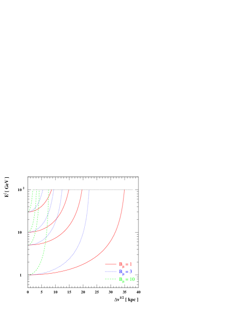
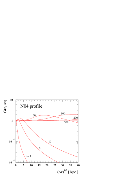
Figure 24: Left: The figure shows the distance $(\Delta v)^{1/2}$ which, on average, a electron covers while losing energy from its energy at emission $E^{\prime}$ and the energy when it interacts $E$, for a few values of $E$: 30 GeV, 10 GeV, 5 GeV and 1 GeV, and for a few values of the magnetic field (in $\mu$G); we are focusing on a WIMP of mass 100 GeV, hence cutting $E^{\prime}<100$ GeV. Right: Green function $\widehat{G}$ as a function of $(\Delta v)^{1/2}$, for a few values of the radial coordinate $r$ (in kpc) and in case the DM halo of Coma is described by a N04 profile with $M_{vir}=0.9\,10^{15}M_{\odot}{\ }h^{-1}$ and $c_{vir}=10$.

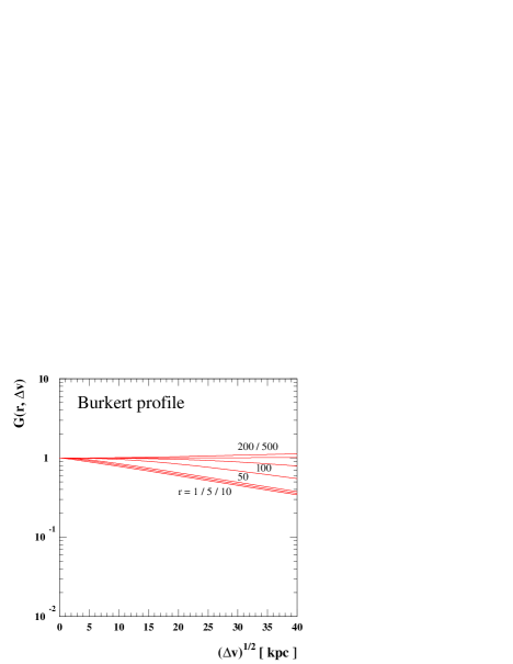
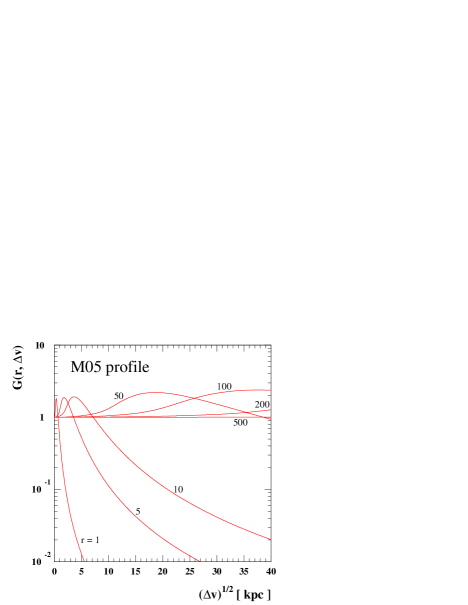
Figure 25: Green function $\widehat{G}$ as a function of $(\Delta v)^{1/2}$, for a few values of the radial coordinate $r$ (in kpc) and in case the DM halo of Coma is described by a cored Burkert profile with $M_{vir}=0.9\,10^{15}M_{\odot}{\ }h^{-1}$ and $c_{vir}=10$ and for the Diemand et al. profile with the same parameters.

As a sample case, in Fig. 24 we consider a WIMP mass $M_{\chi}=100$ GeV and sketch the mapping between the energy $E^{\prime}\in(E,M_{\chi})$, with $E$ some reference energy after diffusion, and the square root of $\Delta v=v-v^{\prime}\equiv v(E)-v(E^{\prime})$, for a few values of $E$ and of the mean magnetic field $B_{\mu}$. We find as largest value $(\Delta v)^{1/2}\sim 35$ kpc, corresponding to $E=1$ GeV and $B_{\mu}=1$ $\mu$G; the maximum value of $\Delta v$ diminishes rapidly when increasing $E$ or $B_{\mu}$.

On the right-hand side of Fig. 24, we plot $\widehat{G}$ as a function of $(\Delta v)^{1/2}$ for a few values of the radial coordinate $r$ and in case the DM halo of Coma is described by a N04 profile. In the very central part of the halo, there are significant departures of the value of $\widehat{G}$ from unity, on scales $(\Delta v)^{1/2}$ at which, for the given radius $r$, the mean squared value of the DM profile is significantly different from the square of the value of the profile at $r$. Note, however, that this effect is confined in the innermost region of the cluster, corresponding to an angular size of $\approx 1-2$ arcmin. We then expect that taking into account spatial diffusion will modify only slightly the predictions for the radio surface brightness distribution from moderate to large radial distances in Coma.

In Fig. 25, we plot $\widehat{G}$ as a function of $(\Delta v)^{1/2}$ for the same values of the radial coordinate $r$ as in Fig. 24 but now in case the DM halo of Coma is described by a Burkert profile. It is clear that departures from unity are essentially negligible even in the inner portion of the halo and, hence, spatial diffusion can be safely neglected for all practical purposes in this case.

To get a more physical insight on the reason why spatial diffusion can be neglected, it is useful to consider the following qualitative solution (see, e.g., Colafrancesco (2005)) for the average electron density

$${dn_{e}(E,r)\over dE}\approx[Q_{e}(E,r)\tau_{loss}]\times{V_{s}\over V_{s}+V_{o}}\times{\tau_{D}\over\tau_{D}+\tau_{loss}}$$ (81)

which resumes the relevant aspects of the transport equation (Eq. 64). Here, $V_{s}\propto R^{3}_{h}$ and $V_{o}\propto\lambda^{3}(E)$ are the volumes occupied by the DM source and the one occupied by the diffusing electrons which travel a distance $\lambda(E)\approx[D(E)\cdot\tau_{loss}(E)]^{1/2}$ before loosing much of their initial energy. The relevant time scales in Eq. (64) are the diffusion time-scale, $\tau_{D}\approx R^{2}_{h}/D(E)$, and the energy loss time-scale $\tau_{loss}=E/b_{e}(E)$, where $D$ is again the diffusion coefficient for which we can assume the generic scaling $D(E)=\tilde{D}_{0}(E/E_{0})^{\gamma}B^{-\gamma}$, and $b(E)$ the electron energy loss per unit time at energy $E$.

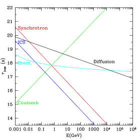
Figure 26: A comparison among the time scales for the energy losses due to various mechanisms (as labeled in the figure) and the time scale for diffusion (black solid curve) in a cluster of size $r_{h}=1$ Mpc. A uniform magnetic field of value $B=1\mu$G and a thermal gas density $n=1.3\cdot 10^{-3}$ cm^-3 have been assumed in the computations.

For $E>E_{*}=(\tilde{D}_{0}E_{0}/R^{2}_{h}b_{0}B_{\mu}^{\gamma})^{1/(1-\gamma)}$ (for simplicity we have kept leading terms only, implementing $b(E)\simeq b_{0}(B_{\mu})(E/GeV)^{2}+b_{Coul}$), the condition $\tau_{D}>\tau_{loss}$ (and consistently $\lambda(E)<R_{h}$) holds, the diffusion is not relevant and the solution of Eq. (64) is $dn_{e}/dE\sim Q_{e}(E,r)\tau_{loss}$ and shows an energy spectrum $\sim Q(E)\cdot E^{-1}$. This situation ($\lambda(E)<R_{h}$, $\tau_{D}>\tau_{loss}$) applies to the regime of galaxy clusters which we discuss here for the specific case of Coma, as one can see from Fig. 26.
For $E<E_{*}$, the condition $\tau_{D}<\tau_{loss}$ (and consistently $\lambda(E)>R_{h}$) holds, the diffusion is relevant and the solution of Eq. (64) is $dn_{e}/dE\sim[Q_{e}(E,r)\tau_{D}]\times(V_{s}/V_{o})$ and shows an energy spectrum $\sim Q(E)\cdot E^{(2-5\gamma)/2}$ which is flatter or equal to the previous case for reasonable values $\gamma=1/3-1$. This last situation ($\lambda(E)>R_{h}$, $\tau_{D}<\tau_{loss}$) applies to the regime of dwarf galaxies and we will discuss this case more specifically elsewhere (Colafrancesco, Profumo & Ullio (2006)).

Fig.27 shows the energy shape of the electron equilibrium spectra derived in our approach for a ($b\bar{b}$) model with $M_{\chi}=40$ GeV and for a $W^{+}W^{-}$ model with $M_{\chi}=81$ GeV. The astrophysical predictions of these two models will be extensively discussed in the following.

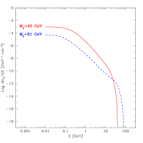
Figure 27: The electron equilibrium spectra calculated at the center of Coma as obtained for a soft spectrum due to a $b\bar{b}$ annihilation final state (solid line, model with $M_{\chi}=40$ GeV) and of a hard spectrum due to a $W^{+}W^{-}$ channel (dashed line, model with $M_{\chi}=81$ GeV).

We notice that the energy losses in the diffusion equation erase almost completely the details of the electron source spectra (see Fig. 7). The equilibrium spectra are generally characterized by three different regions: i) a low-energy plateau at $E\ \raise-2.0pt\hbox{\hbox to0.0pt{\hbox{$\sim$}\hss}\raise 5.0pt\hbox{$<$}\ }0.1$ GeV with a constant value of $dn_{e}/dE$ which remains almost constant down to the electron rest-mass energy; ii) an almost power-law branch at $0.1M_{\chi}\ \raise-2.0pt\hbox{\hbox to0.0pt{\hbox{$\sim$}\hss}\raise 5.0pt\hbox{$<$}\ }E\ \raise-2.0pt\hbox{\hbox to0.0pt{\hbox{$\sim$}\hss}\raise 5.0pt\hbox{$<$}\ }0.5M_{\chi}$ which is steeper in the softer $b\bar{b}$ annihilation final state with respect to the hard spectrum due to a $W^{+}W^{-}$ channel; and iii) a sharp cut-off at the energy corresponding to the neutralino mass which marks the natural maximum energy of the secondary electron spectra. We will show in the next Sect.4 how these three branches of the electron equilibrium spectra will provide observable features in the multi-frequency spectrum of Coma and can, consequently, be used to constrain the neutralino model.

References

- Arnaud et al. (2001) Arnaud, M. et al. 2001, A&A, 365, L67
- Baer et al. (2000) Baer, H., Diaz, M.A., Quintana, P. and Tata, X. 2000, JHEP 0004, 016 [arXiv:hep-ph/0002245].
- Baer et al. (2003) Baer, H., Balazs, C., Belyaev, A:, Krupovnickas, T. and Tata, X. 2003, JHEP, 0306, 054 [arXiv:hep-ph/0304303] and references therein.
- (4) H. Baer, T. Krupovnickas, S. Profumo and P. Ullio, JHEP 0510 (2005) 020 [arXiv:hep-ph/0507282].
- Baer and Profumo (2005) H. Baer and S. Profumo, JCAP 0512 (2005) 008 [arXiv:astro-ph/0510722].
- (6) H. Baer, A. Mustafayev, S. Profumo, A. Belyaev and X. Tata, Phys. Rev. D 71, 095008 (2005) [arXiv:hep-ph/0412059]; H. Baer, A. Mustafayev, S. Profumo, A. Belyaev and X. Tata, arXiv:hep-ph/0504001, JHEP, in press;
- Baltz, (2004) Baltz, E.A. 2004, eConf C040802, L002 [arXiv:astro-ph/0412170].
- Baltz & Edsjo (1998) Baltz, E.A. and Edsjo, J. 1999, Phys. Rev. D 59, 023511 [arXiv:astro-ph/9808243].
- Baltz & Wai (2004) Baltz, E.A. and Wai, L. 2004, Phys. Rev. D 70, 023512 [arXiv:astro-ph/0403528].
- Bardeen et al. (1986) Bardeen, J.M., Bond, J.R., Kaiser, N. and Szalay, A.S. 1986, ApJ, 304, 15
- Battaglia et al. (2003) Battaglia, M., De Roeck, A., Ellis, J.R., Gianotti, F., Olive, K.A. and Pape, L. 2004, Eur. Phys. J. C, 33 273 [arXiv:hep-ph/0306219].
- Bennet et al. (2003) Bennett, C.L. et al. 2003, ApJS, 148, 1
- Bergstrom & Snellman (1988) Bergstrom, L. and Snellman, H. 1988, Phys. Rev. D, 37, 3737
- Bergstrom & Ullio (1997) Bergstrom, L. and Ullio, P. 1997, Nucl. Phys. B, 504, 27 [arXiv:hep-ph/9706232].
- Bergstrom et al. (1998) Bergstrom, L., Edsjo,J., Gondolo, P. and Ullio, P. 1999, Phys. Rev. D, 59, 043506 [arXiv:astro-ph/9806072].
- Bergstrom (2000) Bergstrom, L. 2000, Rept. Prog. Phys. , 63, 793 [arXiv:hep-ph/0002126].
- Bertone et al. (2004) Bertone, G., Hooper, D. and Silk, J. 2005, Phys. Rept. 405, 279 [arXiv:hep-ph/0404175].
- Blasi & Colafrancesco (1999) Blasi, P. and Colafrancesco, S. 1999, AstroParticle Physics, 12, 169
- Binney & Mamon (1982) Binney J. and Mamon, G.A. 1982, MNRAS, 200, 361.
- Birkinshaw (1999) Birkinshaw, M. 1999, Phys. Report, 310, 97
- Bonamente et al. (2003) Bonamente, M. et al 2003, ApJ, 585, 722
- Bowyer et al. (2004) Bowyer, S., Korpela, E.J., Lampton, M. and Jones, T.W. 2004, ApJ, 605, 168
- Bottino et al. (2003) A. Bottino, F. Donato, N. Fornengo and S. Scopel, 2003, Phys. Rev. D, 68, 043506 [arXiv:hep-ph/0304080].
- Briel et al. (1992) Briel, U.G., Henry, J.P. and Böhringer, H. 1992, A&A, 259, L31.
- Brunetti et al. (2004) Brunetti, G. et al. 2004, MNRAS, 450, 1174
- Bryan & Norman (1998) Bryan, G. and Norman, M. 1998, ApJ, 495, 80
- Bullock et al. (2001) Bullock, J.S. et al. 2001, MNRAS, 321, 559
- Burkert (1995) Burkert, A. 1995, ApJ, 447, L25; P. Salucci and A. Burkert 2000, ApJ, 537, L9.
- Chung et al. (2003) Chung, D.J.H., Everett, L.L., Kane, G.L., King, S.F., Lykken, J. and Wang, L.T. 2005, Phys. Rept. 407, 1 [arXiv:hep-ph/0312378].
- Colafrancesco (2003) Colafrancesco, S. 2003, in Frontiers of Cosmology, A. Blanchard & M. Signore Eds., p.75 and p.85
- Colafrancesco (2004) Colafrancesco, S. 2004, A&A, 422, L23
- Colafrancesco (2005) Colafrancesco, S. 2005, in proceedings of the IAUC198 ”Near-Field Cosmology with Dwarf Elliptical Galaxies”, H. Jerjen & B. Binggeli Eds., p.
- Colafrancesco (2006) Colafrancesco, S. 2006, Journal of Physics G: Nuclear and Particle Physics, in press
- Colafrancesco et al. (1994) Colafrancesco, S. et al. 1994, ApJ, 433, 454
- Colafrancesco et al. (1997) Colafrancesco, S. et al. 1994, ApJ, 479, 1