Formation of Structure in Molecular Clouds: A Case Study

Abstract

Molecular clouds (MCs) are highly structured and “turbulent”. Colliding gas streams of atomic hydrogen have been suggested as a possible source of MCs, imprinting the filamentary structure as a consequence of dynamical and thermal instabilities. We present a 2D numerical analysis of MC formation via converging HI flows. Even with modest flow speeds and completely uniform inflows, non-linear density perturbations as possible precursors of MCs arise. Thus, we suggest that MCs are inevitably formed with substantial structure, e.g., strong density and velocity fluctuations, which provide the initial conditions for subsequent gravitational collapse and star formation in a variety of galactic and extragalactic environments.

1. Motivation

Molecular clouds (MCs) in our Galaxy are complex and highly-structured, with broad, non-thermal linewidths suggesting substantial turbulent motion (Falgarone & Philips, 1990; Williams et al., 2000). Thus, MCs very likely are not static entities and might not necessarily be in an equilibrium state, but their properties could well be determined by their formation process. The importance of initial conditions for cloud structure is emphasized by observational and theoretical evidence for short cloud ”lifetimes” (Ballesteros-Paredes et al., 1999; Elmegreen, 2000; Hartmann et al., 2001; Hartmann, 2002).

Flows are ubiquitous in the interstellar medium (ISM) due to the energy input by stars - photoionization, winds, and supernovae. In principle, they can pile up atomic gas to form MCs. Shock waves propagating into the warm ISM will fragment in the presence of thermal instability and linear perturbations (Koyama & Inutsuka, 2000, 2002, 2004b; Hennebelle & Pérault, 1999, 2000) and allow H₂-formation within a few Myrs (Bergin et al., 2004) in a plane-parallel geometry. We envisage the colliding flows less as e.g. interacting shells, but as (more or less) coherent gas streams from turbulent motions on scales of the order of the Galactic gaseous disk height (Ballesteros-Paredes et al., 1999; Hartmann et al., 2001). Parametrizing the inflows as a ram pressure allowed Hennebelle et al. (2003, 2004) to study the fragmentation and collapse of an externally pressurized slab.

In this paper we present a study of the generation of filaments and turbulence in atomic clouds – which may be precursors of MCs – as a consequence of their formation process, extending the model of large-scale colliding HI-flows outlined by Ballesteros-Paredes et al. (1999) and Burkert (2004). We discuss the dominant dynamical and thermal instabilities leading to turbulent flows and fragmentation of an initially completely uniform flow. Resulting non-thermal linewidths in the cold gas phases (the progenitors of MCs) reproduce observed values, emphasizing the ease with which turbulent and filamentary structures can be formed in the ISM.

This study is a ”proof of concept”, discussing the dominant instabilities leading to non-linear density perturbations and quantifying the timescales that are necessary to reach conditions under which molecules – and eventually stars – could form. Since turbulence is thought to be one of the main agents controlling star formation (Larson, 1981; Mac Low & Klessen, 2004; Elmegreen & Scalo, 2004), and consequent density fluctuations surely are crucial to gravitational fragmentation, star formation theory can benefit from a better understanding of the structure initially present in MCs. Detailed aspects and parameter studies will be presented in a forthcoming paper (Heitsch et al., 2005).

2. Physical Mechanisms

We restricted the models to hydrodynamics including thermal instabilities, leaving out the effects of gravity and magnetic fields. Gravity would eventually lead to further fragmentation, and magnetic fields would be expected to have a stabilizing effect. For this regime, then, we identify three relevant instabilities:

(1) The Non-linear Thin Shell Instability (NTSI, Vishniac, 1994) arises in a shock-bounded slab, when ripples in a two-dimensional slab focus incoming shocked material and produce density fluctuations. The growth rate is $\sim c_{s}k(k\Delta)^{1/2}$, where $c_{s}$ is the sound speed, $k$ is the wave number along the slab, and $\Delta$ is the amplitude of the spatial perturbation of the slab. Numerical studies focused on the generation of substructure via Kelvin-Helmholtz-modes (Blondin & Marks, 1996), on the role of gravity (Hunter et al., 1986) and on the effect of the cooling strength (Hueckstaedt, 2003). Walder & Folini (1998, 2000) discussed the interaction of stellar winds, and Klein & Woods (1998) investigated cloud collisions. The latter authors included magnetic fields, albeit only partially.

(2) The flows deflected at the slab will cause Kelvin-Helmholtz Instabilities (KHI), which have been studied at great length analytically and numerically. If the velocity profile across the shear layer is given by a step function, and if the densities are constant across the layer, the growth rate is $k\Delta U$, where $\Delta U$ is the velocity difference. If aligned with the flow, magnetic tension forces can stabilize against the KHI.

(3) The Thermal Instability (TI, Field, 1965) rests on the balancing of heating and cooling processes in the ISM. The TI develops an isobaric condensation mode and an acoustic mode, which – under ISM-conditions – is mostly damped. The condensation mode’s growth rate is independent of the wave length, however, since it is an isobaric mode, smaller perturbations will grow first (Burkert & Lin, 2000). A lower growth scale is set by heat conduction, whose scale needs to be resolved (Koyama & Inutsuka, 2004a). The signature of the TI are fragmentation and clumping as long as the sound crossing time is smaller than the cooling time scale. The TI can drive turbulence in an otherwise quiescent medium (Audit & Hennebelle, 2005) – even continuously, if an episodic heating source is available (Kritsuk & Norman, 2002a, b).

3. Numerical Method

All three instabilities grow fastest or at least first on the smallest scales. This poses a dire challenge for the numerical method. We chose a method based on the 2nd order BGK formalism (Prendergast & Xu, 1993; Slyz & Prendergast, 1999; Heitsch et al., 2004; Slyz et al., 2005), allowing control of viscosity and heat conduction. The statistical properties of the models are invariant under changes of viscosity, heat conduction and grid resolution, although the flow patterns change in detail — as to be expected in a turbulent environment (Heitsch et al., 2005). The linear resolution varies between $512$ and $2048$ cells. The heating and cooling rates are restricted to optically thin atomic lines following Wolfire et al. (1995), so that we are able to study the precursors of MCs up to the point when they could form H₂. Dust extinction becomes important above column densities of $N(\mbox{HI})\approx 1.2\times 10^{21}$cm^-2, which are reached only in the dense cold regions of the models. Thus, we can use the unattenuated UV radiation field for grain heating (Wolfire et al., 1995) for most of the simulation domain, expecting substantial uncertainties in cooling rates only for the densest regions. The ionization degree is derived from a balance between ionization by cosmic rays and recombination, assuming that Ly $\alpha$ photons are directly reabsorbed.

Two opposing, uniform, identical flows in the $x$-$y$ computational plane initially collide head-on at a sinusoidal interface with wave number $k_{y}=1$ and amplitude $\Delta$. The incoming flows are in thermal equilibrium. The system is thermally unstable for densities $1\lesssim n\lesssim 10$cm^-3. The cooling curve covers a density range of $10^{-2}\leq n\leq 10^{3}$ cm^-3 and a temperature range of $30\leq T\leq 1.8\times 10^{4}$ K. The box side length is $44$pc. Thus, Coriolis forces from Galactic rotation are negligible. For a interface with $\Delta=0$, a cold high-density slab devoid of inner structure would form. The onset of the dynamical instabilities thus can solely be controlled by varying the amplitude of the interface perturbation. This allows us to test turbulence generations under minimally favourable conditions.

Model series B has $n_{0}=1.0$cm^-3 and $T_{0}=2.5\times 10^{3}$K, series C has $n_{0}=0.5$cm^-3 and $T_{0}=5.3\times 10^{3}$K. The amplitude of the interface perturbation corresponds to $2.5$% of the box length, i.e. $1.1$pc in the horizontal direction. The second digit of the model name gives the Mach number of the inflow. The inflow velocity varies between $6<v_{in}<17$ km s^-1.

4. Results

We chose to present a few models containing the salient features of cloud formation via colliding flows. We ask how hard it is to generate non-linear turbulent density perturbations in an otherwise uniform flow.

4.1. Dominant Instabilities

The structures generated in colliding flows depend strongly on the initial parameters (Fig. 1), as a result of the dominating instability. This is not surprising, since all three instabilities at work have different signatures. For high-density, low-velocity inflows (model B1, upper left panel), the TI dominates and leads to fast cooling, manifested in a coherent slab of cold gas. This situation comes closest to the 1D plane-parallel slab.

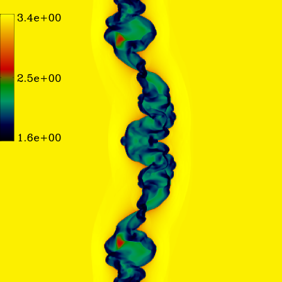
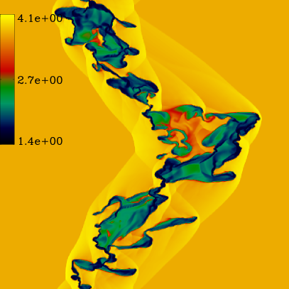
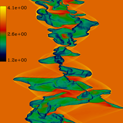
Figure 1.— Temperature maps ($\log T$ in K) for models representative of the dominating instability (see text). From upper left to lower right: B1 (TI), C1 (KHI), C2, (KHI+NTSI), B3 (NTSI).

Reducing the density (model C1, upper right) leads to slightly less efficient cooling, thus giving the dynamical instabilities time to work, in this case dominated by the KHI. The eddies are visible at the flanks of the initial slab. Increasing the inflow speed while keeping all other parameters fixed increases the vertical $x$-momentum transport, so that for model C2 (lower left), the NTSI will arise. Its typical signature are long strands of denser (and colder) gas predominantly along the flow direction (Hueckstaedt 2003). The KHI modes that are still discernible here have vanished in model B3. Here, the NTSI dominates the dynamics almost completely. Oblique colliding flows (not shown) lead to a nearly instantaneous break-up of the initial slab, because they excite KHI modes at the scale of the initial, non-linear perturbation. The NTSI dominates more and more with higher Mach numbers (up to Mach $4$, not shown). This morphological discussion will be quantified in Heitsch et al. (2005).

Despite the symmetric initial conditions, all models develop large-scale asymmetries, resulting from an amplification of slight differences at machine accuracy between the upper and lower half of the domain. The main culprit is the strong cooling. Without cooling (i.e. for an adiabatic or isothermal equation of state), or for 1D problems with cooling, the code preserves perfect symmetry.

4.2. Mass Distribution

Figure 2 shows the mass spectrum of cores. Cores are defined as coherent regions with densities $n>100$cm^-3. Each of the histograms comprises approximately $50$ cores. The dashed line denotes a spectral index of $-1.7$, as observed for observed molecular cores (Heithausen et al., 1998). The resolution limit for both histograms lies at $1.8\mbox{M}_{\odot}$. Note that (a) these ”cores” correspond to cold HI regions, not molecular cores, and that (b) the masses are per length in our 2D models. A direct comparison between these 2D spectra and observed 3D mass spectra requires assumptions concerning what structures the filaments would correspond to in three dimensions. Assuming that the probability density functions are the same for 2D and 3D, the mass spectra are expected to be flatter in 3D (Chappell & Scalo, 2001).

Figure 2.— Left: Mass-histogram of objects with densities $n>100$cm^-3, i.e. likely precursors of molecular fragments, for models C2 and B3. The dashed line denotes a power law with exponent $-1.7$. The resolution limit is $M_{r}=1.8$M_⊙. Right: Histogram of the local Jeans number $L/\lambda_{J}$ for the cold regions, for models C2 and B3. Clearly, none of the dense objects would be gravitationally bound.

Would these cold cores be gravitationally unstable? Although the models do not include self-gravity, we can estimate the thermal Jeans length $\lambda_{J}\equiv(\pi/(G\rho))^{1/2}c_{s}$ and its turbulent counterpart $\lambda_{t}\equiv(\pi/(G\rho))^{1/2}\langle v^{2}\rangle^{1/2}$. The ratio of the cores size over the core’s Jeans length $n_{J}\equiv L/\lambda_{J}<1$, i.e., none of the cores would be gravitationally unstable (Fig.2, right). Since $\lambda_{J}\propto T^{1/2}/(P/T)^{1/2}\propto T$ for an isobaric contraction, the histogram of Figure 2 (right) would shift by a factor of $3$ to larger Jeans masses if we cooled the gas down to $T\approx 10$K, thus still yielding Jeans-stable objects. The core size is determined by the geometric mean of the longest and shortest radius.

However, if we determine the ”global” Jeans number of the cold gas — given by the thickness of the slab over the global Jeans length derived from the mean density and temperature in the cold gas — after $10$Myrs for model B3 and $15$Myrs for model C2, the length scale of the cold gas $L>\lambda_{J}$, i.e. the ”slab” would become gravitationally unstable without turbulence (Fig. 3). Note that these quantities are global measures in the sense that they do not refer to isolated cold regions. The turbulent Jeans length $\lambda_{t}>L$ for all times and models. Global (i.e. large-scale) gravitational effects could still have a crucial effect on the system (Burkert & Hartmann, 2004), especially once the inflow stops.

Figure 3.— Average length scale (thick lines), turbulent Jeans length (medium lines) and thermal Jeans length (thin lines) for models C2 and B3 against time.

4.3. Linewidths and Kinetic Energy Modes

A primary observable of interstellar clouds is the line-of-sight velocity dispersion $\sigma_{v}$. MCs consistently show non-thermal linewidths of a few km s^-1 (Williams et al., 2000), that – together with temperatures of $T\approx 10$K – are generally interpreted as supersonic turbulence in those clouds. The linewidths in our models are consistent with the observed values (Fig. 4). The ”observed” linewidth is derived from the density-weighted histogram of the line-of-sight velocity dispersion in the cold gas at $T<100$K (filled symbols). Comparing this to the internal linewidth of coherent cold regions (open symbols), we note a marked offset between the two values. The sound speed of the cold gas ranges around $0.8$km s^-1. Thus, the internal velocity dispersions do not reach Mach numbers ${\cal M}>1$. Hence, the ”supersonic” linewidths are a consequence of cold regions moving with respect to each other, but not a result of internal supersonic turbulence in the cold gas which eventually would be hosting star formation. This is consistent with the argument by Hartmann (2002), that because of the ages and small spatial dispersions of young stars in Taurus, their velocity dispersions relative to their natal gas are very likely subsonic. Note that the turbulent linewidths $\sigma_{v}$ amount only to a fraction of the inflow velocity.

Figure 4.— Mean velocity dispersion in cold gas at $T<100$K (filled symbols) and in the cold coherent regions (open symbols) against the inflow velocity.

Figure 5 shows the compressible, the solenoidal and the total specific kinetic energy for the whole domain (left) and for the cold gas ($T<100$K, right). Because of the highly compressible initial conditions, the total specific kinetic energy is dominated by compressible modes. However, within the bounding shocks, the highly compressible inflows are converted efficiently into solenoidal motions. Note that because of the 2D geometry, the ratio of solenoidal over compressible kinetic energy is only a lower limit. An extension of Figure 5 to radiative losses and internal energy allows us to estimate the overall efficiency of turbulence generation in MCs (Heitsch et al., 2005).

Figure 5.— Specific kinetic energy fraction against time for models C2 and B3, split up into compressional, solenoidal and total specific kinetic energy. Left: For the whole domain. Right: for the cold gas ($T<100$K). The specific kinetic energy is normalized to the value at $t=0$.

5. Summary

Even for completely uniform inflows, we have shown that the combination of dynamical and thermal instabilities efficiently generates non-linear density perturbations that seed structure of eventual MCs. There is a direct correlation between the morphology of the resulting clouds and the dominating instability.

While our ”cloud” would be gravitationally unstable, the isolated cold regions would still be stable against gravity. Fragmentation and turbulent mixing driven by the incoming warm gas would prevent the global collapse of the cloud – under the caveat that a finite extent of the cloud in the vertical direction might lead to edge effects resulting in collapse (Burkert & Hartmann, 2004). Linewidths reached in the cold gas are consistent with observed values of a few km s^-1 (Fig 4) and reach only a fraction of the inflow speed. The internal linewidths, however, are generally subsonic. Thus, the label ”supersonic turbulence” refers to the velocities with respect to the cold gas, but does not necessarily give a hydrodynamically accurate description of the cold gas.

Although we adopted a specific cooling curve and thus set the physical regime for our models, we expect the mechanism to work on a variety of scales. The surface density of the cold gas should give us a rough estimate of the amount of stars forming later on. Even though the cold gas mass depends strongly on the turbulent evolution of the slab, it correlates strongly with the inflow momentum. In this sense, colliding flows not only could explain the rather quiescent star formation events as in Taurus, but would be a suitable model for generating star bursts in galaxy mergers.

References

- Audit & Hennebelle (2005) Audit, E., Hennebell, P. 2005, A&A, 433, 1
- Ballesteros-Paredes et al. (1999) Ballesteros-Paredes, J., Hartmann, L., Vázquez-Semadeni, E. 1999, ApJ, 527, 285
- Bergin et al. (2004) Bergin, E. A., Hartmann, L. W., Raymond, J. C., Ballesteros-Paredes, J. 2004, ApJ, 612, 921
- Blondin & Marks (1996) Blondin, J. M., Marks, B. S. 1996, New Ast., 1, 235
- Burkert & Hartmann (2004) Burkert, A., Hartmann, L. 2004, ApJ, 616, 288
- Burkert & Lin (2000) Burkert, A., Lin, D. N. C. 2000, ApJ, 537, 270
- Burkert (2004) Burkert, A. 2004, ASP Conf. Ser. 322: The Formation and Evolution of Massive Young Star Clusters, 322, 489
- Chappell & Scalo (2001) Chappell, D., Scalo, S. 2001, MNRAS, 325, 1
- Elmegreen (2000) Elmegreen, B. G. 2000, ApJ, 530, 277
- Elmegreen & Scalo (2004) Elmegreen, B. G., Scalo, J. 2004, ARAA, 42, 211
- Falgarone & Philips (1990) Falgarone, E., Philips, T. G. 1990, ApJ, 359, 344
- Field (1965) Field, G. B. 1965, ApJ, 142, 531
- Hartmann et al. (2001) Hartmann, L., Ballesteros-Paredes, J., Bergin, E. A. 2001, ApJ, 562, 852
- Hartmann (2002) Hartmann, L. 2002, ApJ, 578, 914
- Heithausen et al. (1998) Heithausen, A., Bensch, F., Stutzki, J., Falgarone, E., Panis, J. F. 1998, A&A, 331, L65
- Heitsch et al. (2004) Heitsch, F., Zweibel, E. G., Slyz, A. D., & Devriendt, J. E. G. 2004, ApJ, 603, 165
- Heitsch et al. (2005) Heitsch, F., Slyz, A. D., Devriendt, J. E. G., Hartmann, L., Burkert, A. 2005, in prep.
- Hennebelle & Pérault (1999) Hennebelle, P., Pérault, M. 1999, A&A, 351, 309
- Hennebelle & Pérault (2000) Hennebelle, P., Pérault, M. 2000, A&A, 359, 1124
- Hennebelle et al. (2003) Hennebelle, P., Whitworth, A. P., Gladwin, P. P., & André, P. 2003, MNRAS, 340, 870
- Hennebelle et al. (2004) Hennebelle, P., Whitworth, A. P., Cha, S.-H., & Goodwin, S. P. 2004, MNRAS, 348, 687
- Hueckstaedt (2003) Hueckstaedt, R. M. 2003, New Ast., 8, 295
- Hunter et al. (1986) Hunter Jr., J. H., Sandford II, M. T., Whitaker, R., Klein, R.I. 1986, ApJ, 305, 309
- Klein & Woods (1998) Klein, R. I., Woods, D. T. 1998, ApJ, 497, 777
- Koyama & Inutsuka (2000) Koyama, H., & Inutsuka, S. 2002, ApJ, 532, 980
- Koyama & Inutsuka (2002) Koyama, H., & Inutsuka, S. 2002, ApJ, 564, L97
- Koyama & Inutsuka (2004a) Koyama, H., & Inutsuka, S. 2004, ApJ, 602, L25
- Koyama & Inutsuka (2004b) Koyama, H., & Inutsuka, S. 2004, RMxAC, 22, 26
- Kritsuk & Norman (2002a) Kritsuk, A. G., & Norman, M. L. 2002, ApJ, 569, L127
- Kritsuk & Norman (2002b) Kritsuk, A. G., & Norman, M. L. 2002, ApJ, 580, L51
- Larson (1981) Larson, R. B. 1981, MNRAS, 194, 809
- Mac Low & Klessen (2004) Mac Low, M.-M., & Klessen, R. S. 2004, Reviews of Modern Physics, 76, 125
- Prendergast & Xu (1993) Prendergast, K. H., Xu, K., 1993, J. Comp. Phys., 109, 53
- Slyz & Prendergast (1999) Slyz, A. D., Prendergast, K. H. 1999, A&AS, 139, 199
- Slyz et al. (2005) Slyz, A. D., Devriendt, J. E. G., Bryan, G., & Silk, J. 2005, MNRAS, 356, 737
- Vishniac (1994) Vishniac, E. T. 1994, ApJ, 428, 186
- Walder & Folini (1998) Walder, R., Folini, D. 1998, ApSS, 260, 215
- Walder & Folini (2000) Walder, R., Folini, D. 2000, ApSS, 274, 343
- Williams et al. (2000) Williams, J. P., Blitz, L., & McKee, C. F. 2000, Protostars and Planets IV, 97
- Wolfire et al. (1995) Wolfire, M. G., Hollenbach, D., McKee, C. F., Tielens, A. G. G. M., Bakes, E. L. O. 1995, ApJ, 443, 152