Can bars be destroyed by a central mass concentration? I Simulations

Abstract

We study the effect of a central mass concentration (CMC) on the secular evolution of a barred disc galaxy. Unlike previous studies, we use fully self-consistent 3D $N$-body simulations with live haloes, which are known to be important for bar evolution. The CMC is introduced gradually, to avoid transients. In all cases where the mass of the CMC is of the order of, or more than, a few per cent of the mass of the disc, the strength of the bar decreases noticeably. The amount of this decrease depends strongly on the bar type. For the same CMC, bars with exponential surface-density profile, which formed in a disk-dominated galaxy (MD-type bars), can be totally destroyed, while strong bars with a flat surface-density profile, whose evolution is largely due to the halo (MH-type bars), witness only a decrease of their strength. This decrease occurs simultaneously from both the innermost and outermost parts of the bar. The CMC has a stronger effect on the Fourier components of higher azimuthal wave number $m$, leading to fatter and/or less rectangular bars. Furthermore, the CMC changes the side-on outline from peanut-shaped to boxy or, for massive CMCs, to elliptical. Similarly, side-on initially boxy outlines can be destroyed. The CMC also influences the velocity dispersion profiles. Most of the decrease of the bar strength occurs while the mass of the CMC increases and it is accompanied by an increase of the pattern speed. In all our simulations, the mass of the CMC necessary in order to destroy the bar is at least several per cent of the mass of the disc. This argues that observed super-massive black holes are not likely to destroy pre-existing bars.

1 Introduction

Both bars and central mass concentrations (hereafter CMCs) are features that are present in the majority of disc galaxies. Thus, bars harbouring a CMC should be the rule rather than the exception and it is important to study the effects of the latter on the evolution of the former (and vice versa). Observations in near infrared wavelengths, where the effect of dust is largely suppressed, reveal that between 70% and 90% of all disc galaxies have a bar component (Seigar & James, 1998; Eskridge et al., 2000; Grosbøl, Patsis & Pompei, Grosbøl et al.2004). CMCs – such as massive black holes, central discs, dense central stellar clusters – are very frequent, too.

Super-massive black holes have a mass of the order of $10^{6}-10^{9}\,M_{\odot}$, which correlates with the luminosity, the mass, and, in particular, the velocity dispersion of the hosting bulge (Kormendy & Richstone, 1995; Magorrian et al., 1998; Ferrarese & Merritt, 2000; Gebhardt et al., 2000; Tremaine et al., 2002; McLure & Dunlop, 2002; Marconi & Hunt, 2003). Such correlations lead to a ratio of super-massive black hole mass to bulge mass of the order of $10^{-3}$ (see also Kormendy & Gebhardt, 2001). The mass of the CMC is in fact larger than that of the black hole, since the black hole pulls inwards the bulge and disc material in its immediate neighbourhood and thus forms a cusp, which contributes to the CMC mass (Peebles, 1972; Shapiro & Lightman, 1976; Bahcall & Wolf, 1976; Young, 1980; Goodman & Binney, 1984; Quinlan, Hernquist & Sigurdsson, Quinlan et al.1995; Leeuwin & Athanassoula, 2000).

Compact massive central discs, stellar and/or gaseous, are also examples of CMCs. Gaseous such discs are expected to form particularly frequently in barred galaxies, due to the gas inflow driven by the bar (Athanassoula, 1992b; Wada & Habe, 1992, 1995; Friedli & Benz, 1993; Heller & Shlosman, 1994; Regan & Teuben, 2004). Indeed, observations have shown that large concentrations of molecular gas can be found in many disc galaxies, and particularly in barred ones (Sakamoto et al., 1999; Regan et al., 2001; Helfer et al., 2003). The mass of such components is of the order of $10^{7}-10^{9}\,M_{\odot}$, while their radial extent varies from several tens of parsecs to a couple of kpc. Discy bulges (Athanassoula, 2005b) are examples of mainly stellar such discs (Kormendy & Kennicutt, 2004, and references therein). CMCs can also be central dense stellar clusters, with masses of $10^{6}-10^{8}\,M_{\odot}$.

Orbital-structure studies, aimed at understanding the effect of the CMC on the bar-supporting orbits, were made first in 2D (Hasan & Norman, 1990) and then extended to 3D (Hasan, Pfenniger & Norman, Hasan et al.1993). They include the calculation of the main families of periodic orbits and of their stability. The latter is particularly important, since stable periodic orbits trap around them regular orbits, while unstable periodic orbits generate chaos. These studies showed that with increasing CMC mass or concentration the unstable fraction of the bar-supporting orbits increases, reducing the possibility for barred equilibria.

Orbital-structure studies have thus made the first crucial step in our understanding of the effect of a CMC on a bar by revealing the mechanism by which a CMC could destroy a bar. These studies can inform us whether a given bar model (i.e. density profile and pattern speed) may co-exist with a given CMC. However, the parameter space of bar models is huge and an extensive exploration is neither possible nor meaningful, because nothing will be learned about the evolution of a given bar in presence of a growing CMC.

Such information can only be achieved by appropriate $N$-body simulations, which were pioneered by Norman, Sellwood & Hasan (Norman et al.1996, hereafter NSH). These authors used particles on a grid to represent the (barred) disc, which was exposed to the gravitational field of the CMC and of a spheroidal (bulge-like) component. For both 2D and 3D simulations, NSH found that a CMC of mass 5% of that of the galaxy is sufficient for bar dissolution. In the $N$-body simulations of Shen & Sellwood (2004, hereafter SS) the disc is represented by particles on a 3D cylindrical polar grid and, similarly to NSH, exposed to the gravity of the CMC and of a rigid spherical halo component. These authors found that a CMC mass of a few percent is necessary to destroy the bar, by and large, consistent with the results of NSH. More precisely, in the models displayed in their Fig. 5, a CMC mass of approximately 4% that of the disc was necessary for a hard (compact) CMC and more than 10% for a soft (extended) CMC. They compared two models with different bar strengths and concluded that the strength of the bar hardly influences these numbers.

Recently, Hozumi & Hernquist (1998; 1999; 2005, hereafter HH) re-examined the problem, solving the Poisson equation by expanding the density and the potential in a set of bi-orthonormal basis functions. Their approach is 2D, which implies the necessity for a rigid halo potential, similar to NSH & SS. These authors find that a CMC of mass 0.5% of the disc mass is sufficient to destroy the bar. Thus, their limiting CMC mass is an order of magnitude lower than that given by NSH. The difference between their results and those of NSH & SS is surely significant. Indeed, if the mass necessary to destroy a bar is as small as claimed by HH, then the masses of CMCs observed in disc galaxies are sufficient to dissolve observed bars in relatively short time scales. The opposite is true if the NSH & SS picture is correct.

This disagreement between previous studies, as well as their lack of realism in modeling the galactic halo, prompted us to revisit the problem. HH argued that the differences between the two sets of simulations are due to the different initial density distributions in the disc, since they use an exponential disc, while NSH & SS employed a Kuzmin-Toomre disc (Kuzmin, 1956; Toomre, 1963). HH argue that, since the latter is more centrally concentrated than the former, the CMC could influence a larger fraction of the disc mass and thus achieve bar dissolution easier. However, preliminary simulations (, Athanassoula et al.2003) showed that bars are rather robust, and so we opted for an exponential disc model which is known to represent well the observed light distribution of disc galaxies (Freeman, 1970). This may give a better chance for the CMC to destroy the bar and allows us to check whether indeed the initial density distribution in the disc is of crucial importance for the result. We employ a Poisson solver different from both types previously used in this problem, namely a tree code described in section 2.2.

Unlike the previous studies, we use a live halo in our simulations, which makes them fully self-consistent. This has been shown to be essential for bar formation in presence of a strong halo component. Indeed, Athanassoula (2002, hereafter A02) compared two simulations with initially identical disc components and haloes of identical mass distribution. In one case the halo was rigid (represented as an imposed spherical potential) and in the other it was composed of about $10^{6}$ particles. The difference between the evolution in the two cases is stunning (Fig. 1 of A02). In the first case, the disc formed only a minor oval confined to the centre-most parts of the disc, while in the second case it grew a strong bar with very realistic observed properties (Athanassoula & Misiriotis, 2002, hereafter AM02). This important difference is due to the fact that the angular momentum absorption by the halo is artificially suppressed in one of the two cases, while in the other it is allowed to freely take place (for a comprehensive discussion of the effect of the halo on the angular momentum exchange see Athanassoula, 2003, hereafter A03).

The paper is organised as follows. In section 2 we present our numerical methods and our simulations. Sections 3 and 4 describe the evolution before and after the introduction of the CMC, respectively. We discuss our results and conclude in section 5.

2 $N$-body simulations

We first follow the formation and evolution of a bar in two bar-unstable discs. We choose a time after the initial fast bar formation period and during the phase of slow secular evolution. At this time we start growing a CMC in the centre of the disc. The various steps in this work are described in the following subsections.

2.1 Initial conditions

The models are composed of a disc and a halo component. The disc has an initial volume density profile

$$\rho_{\mathrm{d}}(R,z)=\frac{M_{\mathrm{d}}}{4\pi R_{d}^{2}z_{0}}\;\exp(-R/R_{\mathrm{d}})\;\mathrm{sech}^{2}(z/z_{0}),$$ (1)

where $R$ is the cylindrical radius, $M_{\mathrm{d}}$ is the disc mass and $R_{\mathrm{d}}$ and $z_{0}$ are the disc radial and vertical scale-lengths, respectively. The initial halo density profile is

$$\rho_{h}(r)=\frac{M_{\mathrm{h}}}{2\pi^{3/2}}\;\frac{\alpha}{r_{\mathrm{c}}}\;\frac{\exp(-r^{2}/r_{\mathrm{c}}^{2})}{r^{2}+\gamma^{2}},$$ (2)

where $r$ is the radius, $M_{\mathrm{h}}$ is the halo mass and $\gamma$ and $r_{c}$ are the halo scale-lengths. The former can be considered as the core radius of the halo. The constant $\alpha$ is defined by

$$\alpha=[1-\sqrt{\pi}\,q\,\exp(q^{2})\,(1-\mathrm{erf}(q))]^{-1},$$ (3)

where $q=\gamma/r_{\mathrm{c}}$ (Hernquist, 1993). Information on how the initial conditions were set up can be found in Hernquist (1993) and AM02. Both simulations have $M_{\mathrm{d}}=1$, $R_{\mathrm{d}}=1$, $z_{0}=0.2$, $M_{\mathrm{h}}=5$ and $r_{\mathrm{c}}=10$. The first one has a halo with a small core ($\gamma=0.5$) and is thus, following the definition of AM02, MH-type. The second one has a halo with a large core ($\gamma=5$) and is thus of MD-type (AM02). The discs of the two simulations have $Q=1.4$ and 1, respectively, where $Q$ is the stability parameter introduced by Toomre (1964).

Our model units of mass and length are simply the disc mass and disc scale length. In order to convert them to $M_{\odot}$ and kpc, we need to set the units of length and mass to values representative of the object in consideration, a barred galaxy. AM02 used a length unit of 3.5 kpc and a mass unit of $5\times 10^{10}\,M_{\odot}$. With $G=1$, this implies that the model unit of velocity is 248 km s^-1 and the model unit of time is $1.4\times 10^{7}\,$yr. Thus, time 400 corresponds to $5.6\times 10^{9}\,$yr. This choice, however, is in no way unique, and we can choose quite different values. For example, we can use a smaller length unit since the scale-length of the disc increases with time (O’Neill & Dubinski, 2003; Valenzuela & Klypin, 2003) and thus the initial length unit could be chosen to be 2 kpc. Because of this rather wide range of possibilities, we will restrict ourselves to model units and leave it to the readers to convert units according to their needs.

2.2 $N$-body simulations

For the simulations described in this paper, we used the publicly available $N$-body code gyrfalcON, which employs the tree-based force solver falcON (Dehnen, 2000a, 2002). Unlike the standard Barnes & Hut (1986) tree code, which has complexity $\mathcal{O}(N\log N)$, falcON uses cell-cell interactions, has complexity $\mathcal{O}(N)$, and is about ten times faster at comparable accuracy. Some of the simulations were run with a proprietary version of the code, which uses the SSE instruction set supported on X86 chips. These instructions allow a substantial speed-up for the computation of body-body forces via direct summation. This method is used within and between small cells and results in a gain of a factor of $\sim 2$ for this part of the code. The total gain for the force computation for $N\sim 10^{6}$ bodies (including the tree build) is about 25%.

In all $N$-body simulations it is necessary to use a softening kernel in order to avoid excessive noise and diverging forces. A Plummer (1911) softening, which has density kernel $\propto(\varepsilon^{2}+r^{2})^{-5/2}$, has been used in most simulations made so far. This, however, has the disadvantage that the softened force converges relatively slowly to the Newtonian force (Athanassoula et al., 2000; Dehnen, 2001), although the difference becomes negligible, and beyond any numerical importance, at large radii. Here we adopt a softening with a density kernel $\propto(\varepsilon^{2}+r^{2})^{-7/2}$ (Dehnen et al., 2004), which converges much faster to the accurate Newtonian force. This is particularly interesting for the problem at hand, as will be discussed in the last section. We adopted a softening length $\varepsilon$ of 0.03, which roughly corresponds to a Plummer softening length of 0.02 (in the sense that the maximum two-body force is the same). A small softening length is useful in this problem, since the CMC will create an increased central concentration of the disc and halo components, and more centrally concentrated structures necessitate a smaller softening length (Athanassoula et al., 2000).

The tree code used in our simulations allows for an approximate interaction (as opposed to the direct summation force) between two tree nodes (cells or single bodies) only if their critical spheres do not overlap (Dehnen, 2000a, 2002). The critical spheres are centred on the centre of mass of the nodes and have radii $r_{\mathrm{crit}}=r_{\mathrm{max}}/\theta$, where $r_{\mathrm{max}}$ is the radius containing all particles in the node and $\theta$ the tolerance parameter (opening angle). In our simulations we use $\theta=0.5$.

In order to have sufficiently small time steps in the area around the CMC, we used adaptive time stepping with the block-step scheme (time steps differ by factors of two and are hierarchically nested). In most simulations we used 6 levels, in such a way that the longest time step is $2^{-6}$ and the shortest $2^{-11}$. For the numerically more demanding simulations (with a CMC of very high mass or very small radius) we used 7 levels and a smallest time step of $2^{-12}$. The time step levels are adapted in an (almost) time symmetric fashion to be on average

$$\tau=\min\{f_{a}/a,f_{\Phi}/|\Phi|\},$$ (4)

where $f_{a}$ and $f_{\Phi}$ are constants, $a$ is the modulus of the acceleration and $\Phi$ is the potential. We adopted $f_{a}$ = 0.01 and $f_{\Phi}$ = 0.015, thus ensuring that the smallest time step bin contains of the order of a few percent of the particles.

We model the disc with 200 000 and the halo with roughly 1000 000 particles. With these settings, the energy conservation after the CMC growth (during CMC growth energy is not conserved) was always better than one part in 1 000, and, in most cases, of the order of a couple of parts in 10 000.

2.3 The CMC

Following previous studies (NSH & SS), we model the CMC by a Plummer sphere of potential

$$\Phi_{\mathrm{CMC}}(r)=-\frac{GM(t)}{\sqrt{r^{2}+r_{\mathrm{CMC}}^{2}}},$$ (5)

where $M(t)$ is the mass of the CMC at time $t$ and $r_{\mathrm{CMC}}$ its radius. In order to avoid transients, the CMC is introduced gradually with

$$\frac{M(t)}{M_{\mathrm{CMC}}}=\left\{\begin{array}[]{r@{\quad:\quad}l}0&t\leq t_{\mathrm{in}}\\ \frac{3}{16}\xi^{5}-\frac{5}{8}\xi^{3}+\frac{15}{16}\xi+\frac{1}{2}&t_{\mathrm{in}}<t<t_{\mathrm{grow}}\\ 1&t\geq t_{\mathrm{grow}}\end{array}\right.$$ (6)

where $\xi=2(t-t_{\mathrm{in}})/t_{\mathrm{grow}}-1$ and $t_{\mathrm{in}}$ is the time at which the CMC is introduced (Dehnen, 2000b). Thus the mass, as well as its first and second derivatives, are continuous functions of $t$. The radius $r_{\mathrm{CMC}}$ of the CMC is kept constant with time. In the following, since we are interested in the time evolution after the CMC is introduced, we measure time from the time when the CMC has been introduced, i.e. from $t_{\mathrm{in}}$.

Some of the software used in the analysis has already been described in AM02 and we refer the reader to that paper for more information. Our runs are listed in Table 1. The first column gives the name of the run and the second one the type of the model. The mass of the CMC, $M_{\mathrm{CMC}}$, its radius, $r_{\mathrm{CMC}}$, and its growth time, $t_{\mathrm{grow}}$, are given in the third, fourth and fifth columns, respectively.

Table 1: Parameters for the CMC

model	initial	$M_{\mathrm{CMC}}$	$r_{\mathrm{CMC}}$	$t_{\mathrm{grow}}$
MH	MH	0.	-	-
MH1	MH	0.05	0.01	100
MH2	MH	0.10	0.01	100
MH3	MH	0.10	0.005	100
MH4	MH	0.20	0.01	100
MH5	MH	0.10	0.01	200
MD	MD	0.	-	-
MD1	MD	0.05	0.01	100
MD2	MD	0.10	0.01	100
MD3	MD	0.10	0.005	100
MD4	MD	0.20	0.01	100
MD5	MD	0.10	0.01	200
MD6	MD	0.04	0.01	100
MD7	MD	0.03	0.01	100
MD8	MD	0.02	0.01	100
MD9	MD	0.01	0.01	100
MD10	MD	0.1	0.1	100
MD11	MD	0.1	0.08	100
MD12	MD	0.1	0.05	100
MD13	MD	0.1	0.02	100

3 Evolution prior to the introduction of the CMC

The formation and evolution of the bar in $N$-body simulations has already been extensively described in the literature. Here we will only summarise very briefly some results from AM02, A02, and A03, which are necessary for discussing the simulations at hand, and will refer the interested reader to these papers for more information (see also Athanassoula, 2005a).

Barred galaxies evolve by re-distributing their angular momentum. This is emitted mainly by near-resonant material in the inner disc and absorbed by near-resonant material in the outer disc and in the halo. The amount of angular momentum that can be emitted and absorbed depends on the amount of near-resonant material and on how dynamically hot/cold this is. Since there is relatively little material in the outer disc, the halo can play a major role in this exchange, even though the material that constitutes it is relatively hot. Thus, bars immersed in massive haloes can grow stronger than bars immersed in weak haloes, and very much stronger than bars immersed in rigid haloes. Models where the halo plays a substantial role in the dynamics within the inner 4 or 5 disc scale lengths, while being also sufficiently cool to absorb considerable amounts of angular momentum were termed MH (for Massive Halo) in AM02. Such models form strong bars. On the contrary, models in which the disc dominates the dynamics within that region form less strong bars and were termed MD (for Massive Disc) in AM02. Due to the considerably different dynamics in the two cases, we decided to study the effect of a CMC in two models, one of MH-type and one of MD-type.

The observable properties of the bars which grow in these two types of models are quite different (see AM02 for a more complete discussion). MH-type bars are stronger (longer, thinner and more massive) than MD-type bars. Viewed face-on, they have a near-rectangular shape, while MD-type bars are more elliptical. Viewed side-on, they show stronger peanuts and sometimes (particularly towards the end of the simulation) even ‘X’ shapes. On the other hand, bars in MD-type models are predominantly boxy when viewed side-on.

Figure 1: Projected density profiles along the bar major and minor axes (solid lines) and azimuthally averaged (dashed lines). The disc is seen face-on. The left panel corresponds to model MH and the right one to model MD, both at the time the CMC is introduced.

Fig. 1 shows the projected density radial profiles of the two types of bars seen face-on. The results are in good agreement with what was found by AM02 (see their Fig. 5 and section 5). The radial profile along the major axis of the MD bar decreases with radius without showing any clear change of slope at the end of the bar. On the other hand, for the MH type the profile along the bar major axis is quite different. It has a relatively flat part in the bar region which is followed by a sharp drop at the end of the bar. These two different types of profiles have been also found by observations of barred galaxies. Elmegreen & Elmegreen (1985), using blue and near-infrared surface photometry of a sample of 15 barred galaxies, classified the photometric profiles in the bar region in two classes: the flat ones and the exponentially decreasing ones, i.e. the two types found in our two fiducial simulations. The importance of these two types of profiles for bar destruction will be discussed in the last section.

4 Evolution after introduction of the CMC

4.1 The effect of the CMC

MH-type                                                                     MD-type

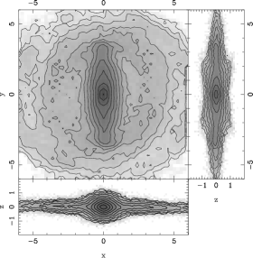
$\Delta T=0$

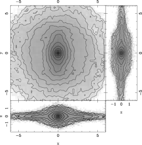
$\Delta T=400$

$M_{\mathrm{CMC}}=0.05$

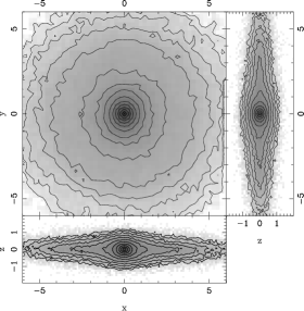
$\Delta T=400$

$M_{\mathrm{CMC}}=0.1$

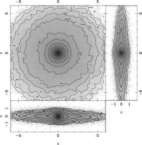
Figure 2: Effect of a CMC on a MH-type (left) and MD-type (right) model. The upper panels show the disc component at the time the CMC is introduced and the others at $\Delta T=$ 400 later. The mass of the CMC is 0.05 for the middle panels and 0.1 for the lower two, while $r_{\mathrm{CMC}}=0.01$ in both cases. Each sub-panel shows one of the three orthogonal views of the disc component. The right sub-panel gives the edge-on side-on view, the lower sub-panel gives the edge-on end-on view and the main sub-panel the face-on view. The projected density of the disc is given by grey-scale and also by isocontours (spaced logarithmically).

4.1.1 MH-type bars

The effect of a CMC on a MH-type bar is shown in the left panels of Fig. 2. The upper left panel shows the three views of the disc component before the CMC is introduced. The face-on view shows a strong bar with ansae at its ends, similar to what is seen in many early types strongly barred galaxies (good examples can be seen on pages 42 and 43 of the Hubble Atlas, Sandage, 1961). Seen side-on, it shows a clear peanut, or mild ‘X’, shape, whose extent is somewhat shorter than the bar, as expected (for a discussion see Athanassoula, 2005b). Seen end-on, the bar can easily be mistaken for a bulge and can only be distinguished from it by kinematical measurements (Bureau & Athanassoula, 2005; Athanassoula, 2005a, b).

The middle and lower panels on the left of Fig. 2 show the disc component a $\Delta T=400$ after the CMC has been introduced. With the units proposed in section 2.1, this is equivalent to 5.6 Gyrs. The mass of the CMC in these two cases is 0.05 and 0.1, respectively and $r_{\mathrm{CMC}}=0.01$. We note that the smaller of the two masses did not destroy the bar, but made it considerably less strong. In particular, the final bar is considerably shorter. Since its width has not changed considerably, its axial ratio (minor to major axis) has become considerably larger. The heaviest of the two CMCs has also not destroyed the bar, although its mass is as much as 10% of that of the disc. The resultant bar, however, is rather short and oval. A CMC with a mass of 0.2 is sufficiently massive to destroy the bar and make the disc near-axisymmetric (not shown here).

          $M_{\mathrm{CMC}}=0$                            $M_{\mathrm{CMC}}=0.05$                                     $M_{\mathrm{CMC}}=0.1$

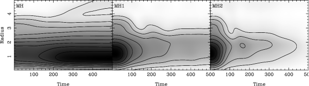
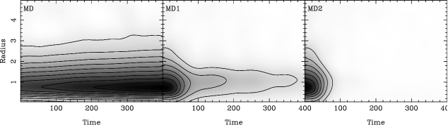
Figure 3: Bar amplitude ($m=2$ Fourier component of the amplitude) as a function of time and radius, for the three MH-type (top) and three MD-type (bottom) simulations snapshots of which are shown in the left and right panels of Fig. 2, respectively. The grey-scale and isocontour levels are set separately in each panel, so as to show best the relevant features. The isocontour levels are spaced linearly and darker shades correspond to higher amplitudes. The name of the simulation is given in the left corner of each panel.

The CMC changes also the vertical structure of the bar. Before the introduction of the CMC and seen side-on, the bar has a peanut-shape, or mild ‘X’-form, with a maximum vertical extent at a distance from the centre roughly equal to three quarters of the bar length and a minimum in between the two maxima. The middle left panel, corresponding to $M_{\mathrm{CMC}}=0.05$, show that the bar seen side-on has a boxy shape, with a roughly constant vertical extent. The radial extent of this boxy feature is roughly the same as that of the peanut before the CMC was introduced. Thus, although the CMC brought a considerable decrease of the bar length seen face-on, it brought little, if any, decrease of the radial extent of the vertically extended feature. The more massive CMC, $M_{\mathrm{CMC}}=0.1$, brings a stronger change to the vertical structure. Seen side-on, the shape is more elliptical than boxy. So the introduction of a CMC changes the side-on outline from peanut to boxy, or, for very massive CMCs, to elliptical. The radial extent of these features, however, does not change much. In the end-on view also, the CMC makes changes in the outline. The vertical extent increases in the central region and also the bulge-like feature becomes considerably more extended radially.

4.1.2 MD-type bars

The right panels of Fig. 2 are similar, but for an initially MD-type bar. Before the CMC is introduced the bar is both fatter and shorter, i.e. less strong than that of the previous example, in agreement with the results of AM02. It also has no ansae. Seen side-on, it has a boxy structure, but no peanut. The middle and lower right panels show the disc component a $\Delta T=400$ after the CMC has been introduced. The mass of the CMC in these two cases is again 0.05 and 0.1, respectively and $r_{\mathrm{CMC}}=0.01$. We note that the introduction of the CMC makes major changes. Seen face-on, the bar has nearly disappeared even for $M_{\mathrm{CMC}}=0.05$, where only close scrutiny allows one to see that the isophotes are not circular, but slightly elongated in what used to be the bar region . For $M_{\mathrm{CMC}}=0.1$, there is no trace of the bar anymore, the isophotes being circular within the measuring errors. Seen side-on, the boxiness has more or less disappeared for $M_{\mathrm{CMC}}=0.05$, and there is definitely no trace left by $M_{\mathrm{CMC}}=0.1$. Thus, judging from the morphology of the three orthogonal views, the models with $M_{\mathrm{CMC}}=0.1$ or 0.05, qualify as an SA galaxy, i.e. a galaxy with no bar. Thus, even moderately light CMC can destroy the bar in MD-type models. This is contrary to what was found above for MH-type models and constitutes an important difference between the two.

To check whether a less massive CMC can still destroy the bar we ran four more simulations with $M_{\mathrm{CMC}}$ equal to 0.04, 0.03, 0.02 and 0.01, respectively. In all four cases the bar is clearly visible by the end of the simulation, although considerably weakened. We also ran simulations with $M_{\mathrm{CMC}}$ = 0.1 and $r_{\mathrm{CMC}}>0.01$ to check whether the bar is destroyed even for CMCs with such large radii. We found that $r_{\mathrm{CMC}}$ has to be at least as large as 0.1 for the bar not to be destroyed.

4.2 The bar strength

4.2.1 The bar strength as a function of time and radius

Figure 3 gives, for six simulations, the amplitude of the $m=2$ (bisymmetric) component of the mass/density distribution as a function of both time and radius. This is a simple measure of the bar strength. The results for higher $m$ values will be discussed in the next subsection. The left panels correspond to two reference simulations in which no CMC has been introduced. They show clearly a secular evolution, during which the bar gets slowly and steadily stronger. We note that the maximum amplitude increases, but also that both the innermost and the outermost parts become gradually more bisymmetric.

Figure 4: Relative amplitude of the $m=2$ (solid line), 4 (dashed line), 6 (dot-dashed line) and 8 (dotted line) Fourier components of the mass/density. The name of the simulation is given in the upper left corner and the time since the introduction of the CMC in the upper right corner of each panel.

Figure 5: As in figure 4, but for MD-type models.

The picture is different for simulations with a CMC. At early times, up to 20 or 30 time units after the CMC has been introduced, the evolution continues more or less as if no CMC had been introduced. This is presumably because the CMC has to reach a limiting mass before its effect can be felt by the bar and/or because the orbits in the bar region take some time to adjust. This time interval is longer in the case of less massive CMCs. After that starts a second time interval, which lasts roughly till the time the CMC reaches its maximum mass. During this second phase the amplitude drops abruptly with time. A third time interval starts after that and lasts till the end of the simulation. Unless the bar has totally disappeared after the end of the second interval, its amplitude continues to decrease in this third phase, but at a considerably slower rate than in the second one. The distinction between the second and the third time interval is sharper for MD-type than for MH-type models and for more massive CMCs. Figure 3 shows clearly that the maximum amplitude decreases steadily with time. But also that both the innermost and the outermost parts of the disc become gradually more axisymmetric. This is in agreement with what is seen in figure 2. Indeed, it was clear there that at $\Delta T=400$ after the CMC was introduced the bar has become shorter and also that the innermost isophotes have become rounder. The corresponding time evolution can be followed in figure 3.

Comparison of the upper and lower panels of Fig. 3 shows that a given CMC can destroy MD-type bars more efficiently than MH-type ones. Also comparison of the central and right rows of panels shows that more massive CMCs are more efficient for bar destruction, as expected.

4.2.2 Higher $m$ values

Fig. 4 shows the amplitude of the relative $m$ = 2, 4, 6, and 8 Fourier components of the mass/density for MH-type simulations. They have been calculated as described in AM02. Before the introduction of the CMC (left panel) all components have high amplitudes. In particular, their maxima are 0.7, 0.48, 0.33 and 0.25, for $m$ = 2, 4, 6 and 8, respectively. The introduction of the CMC brings a considerable decrease of all these values. Thus, for a $M_{\mathrm{CMC}}$ = 0.05 and $\Delta T$ = 400 the maxima of the amplitudes for the various $m$s fall to 0.54 ($m$ = 2), 0.43 ($m$ = 4), 0.32 ($m$ = 6) and 0.25 ($m$ = 8) of the initial maximum values, respectively. For $M_{\mathrm{CMC}}$ = 0.1 and the same time lapse the $m$ = 2 amplitude falls to 0.3 of its initial value, while the other components drop to the noise level.

Fig. 4 quantifies the effect of the CMC and, more importantly, shows that it has a stronger effect on the higher $m$ components. The latter can be understood as follows: As can be seen from the left panel of Fig. 4, before the CMC is introduced the radius at which the relative amplitude has its maximum increases with $m$ and comes closer to the outer regions of the bar. These regions, as we saw in section 4.1 and 4.2.1, are affected first and tend faster to axisymmetry. In this way, the higher $m$ components will be affected before the lower ones. This argument is further re-enforced when we look at the positions of the maxima. For $m=2$ the maximum is at roughly 2.1 and stays there after the CMC has been introduced, as can be seen by comparing the left panel to the middle and right ones. On the other hand the maximum of the $m=4$, and 6 components is roughly at 2.4 at the time the CMC is introduced, and moves to 2.1, i.e. the same radius as that of the $m=2$ maximum, 400 time units after a CMC with $M_{\mathrm{CMC}}=0.05$ is introduced. Since the higher $m$ components are affected less than the lower $m$ ones, the iso-density contours become fatter and/or less rectangular (and thus more elliptical). Fig. 2 confirms this.

Fig. 5 gives similar information, but for MD-type simulations. As already discussed in AM02, MD-type models have lower values of all the amplitudes and also lower values of the relative amplitude of the higher $m$ components than MH-type models. Thus, for MD-types, the CMC destroys the higher $m$ components even for relatively small values of the CMC mass. This is illustrated in Fig. 5, where we show results for two models with $M_{\mathrm{CMC}}$ equal to 0.01 and 0.02, respectively.

4.3 Velocity dispersions along the bar major axis

Figure 6: Velocity dispersion as a function of distance from the centre, as discussed in section 4.3. The left row of panels correspond to MH simulations at the time the CMC is introduced, while the central and right rows of panels correspond to simulations MH₁ and MH₂, respectively. The three components of the velocity dispersion, $\sigma_{x}$, $\sigma_{y}$ and $\sigma_{z}$, are given in the upper, middle and lower rows of panels, respectively. The name of the simulation is given in the upper left corner and the time since the introduction of the CMC in the upper right corner of the upper panels.

Fig. 6 shows the three components of the velocity dispersion as a function of distance from the centre. They have been calculated as described in AM02. Namely, we isolate a thin strip of particles centred on the bar major axis and having a width of 0.07. The distance from the centre is calculated along this strip. In this way, we avoid making an integration along the line of sight, since this would impose the choice of a particular viewing angle. We also bring out clearer the information on the motions of particles near the bar major axis, which is of particular use when comparing with periodic orbit structure. Nevertheless, any comparison with observations can only be rough, since our presentation gives information only on a subset of the orbits.

At the time the CMC is introduced, the velocity dispersions of model MH show features characteristic of MH-type models (see AM02 for a more complete description). The $\sigma_{x}$ component (perpendicular to the bar) has a clear maximum at the centre and two secondary maxima on either side of it. These can be due to orbits trapped around x₁ periodic orbits with loops at their apo-centres, and/or on the superposition of orbits trapped around elliptical and around rectangular shaped periodic orbits. The CMC turns these maxima into plateaus and moves them nearer to the centre. Both effects could be expected. Indeed these maxima are only found for strong bars (AM02), while the CMC has reduced the bar strength. Also these structures are linked to the end of the bar and the CMC makes this shorter (sections 4.1 and 4.2.1). Of course the clearest effect of the CMC is to raise very substantially the central velocity dispersion, and more strongly so for the most massive CMCs.

Figure 7: The upper panels give the pattern speed of the bar as a function of time. For some simulations and times the bar is not sufficiently strong to allow a correct measurement of the pattern speed, so we give no estimates. The lower panels give, for comparison, a measure of the bar strength, also as a function of time. As such a measure we use the maximum value of the amplitude of the $m$ = 2 component of the mass. The left panels refer to a series of simulations with different $M_{\mathrm{CMC}}$ : MD₉ (solid line), MD₈ (dashed), MD₇ (dot-dashed), MD₆ (dashed) and MD₁ (3 dots-dashed). The right panels correspond to a series of simulations with different $r_{\mathrm{CMC}}$ : MD₂ (solid line), MD₁₃ (dashed), MD₁₂ (dot-dashed), MD₁₁ (dashed) and MD₁₀ (3 dots-dashed).

At the time the CMC is introduced, the $\sigma_{y}$ component has a small, but characteristic, minimum at the centre, surrounded closely by two maxima on either side. Since the $\sigma_{y}$ is the component parallel to the bar major axis, this feature should be mainly seen in edge-on barred galaxies which are viewed nearer to end-on than to side-on. The CMC obliterates this feature and creates, instead, a clear central maximum, as for $\sigma_{x}$. The $\sigma_{x}$ and $\sigma_{y}$ components have quite different values at the centre in the case with no CMC. As expected, however, the velocity distribution in the central regions becomes more isotropic in the cases with CMC, and more strongly so for the most massive CMCs.

The MD-type models show no clear characteristic features on their velocity dispersion profiles (see fig. 13 of AM02). Thus the CMC only introduces a sharp maximum at the centre, clear in all three components of the velocity dispersion, as was seen already in the MH-type models.

4.4 CMC radius and growth time

We ran two simulations with smaller values of $r_{\mathrm{CMC}}$ (see Table 1) and found that more centrally concentrated CMCs are more efficient for bar destruction, thus confirming a result already found by (Hasan et al.1993), with orbital calculations, and by SS, with simulations.

We also ran two simulations with a larger value of $t_{\mathrm{grow}}$ (see Table 1) and confirmed a result already found by SS and by HH, namely that the value of $t_{\mathrm{grow}}$ does not influence much the final bar weakening. It only influences the duration of the initial strong decrease. The transition between the initial strong decrease and the later milder one is sharper in simulations with larger $M_{\mathrm{CMC}}$ and/or smaller $r_{\mathrm{CMC}}$ (see bottom panels Fig. 7).

4.5 Pattern speed

NSH mentioned that the introduction of the CMC results in an increase of the bar pattern speed. In order to assess further the effect of the CMC on the bar pattern speed, we measured this quantity in our simulations. This was not always easy, since in many cases the bar amplitude is so weak that the measurement was either not possible, or gave a very uncertain value. In most cases, some smoothing was necessary. Nevertheless, from the cases where the measurement is sufficiently precise, we can clearly see that the pattern speed increases with time, as the bar gets weaker. This is shown, for two sets of MD-type simulations, in Fig. 7 and for MH-type simulations in Fig. 8. For comparison, we also plot a measure of the bar strength as a function of time. As such we have chosen the maximum value of the amplitude of the $m$ = 2 component of the mass. Results found with other measures of the bar strength are similar.

The left panels of Fig. 7 give results from a series of simulations with different values of the mass of the CMC, namely simulations MD₉ ($M_{\mathrm{CMC}}$ = 0.01), MD₈ (0.02), MD₇ (0.03), MD₆ (0.04) and MD₁ (0.05). In the very first 20 time units or so, the bar strength increases, as in simulations with no CMC. During this time, at least in simulations with small CMCs, the pattern speed decreases, again as in simulations with no CMC. This is presumably due to the fact that the CMC has not grown enough to influence the evolution sufficiently to reverse the trend. This reversal indeed occurs at somewhat later times. We note that the bar speed increases noticeably up to time 100, while the CMC mass increases and the bar strength decreases most strongly. At later times there may still be an increase in the pattern speed, but it is very small and the data are too noisy to assess it with any certainty.

The right panels Fig. 7 give similar results, now from a series of simulations with different values of the radius of the CMC, namely simulations MD₂ ($r_{\mathrm{CMC}}$ = 0.01), MD₁₃ (0.02), MD₁₂ (0.05), MD₁₁ (0,08) and MD₁₀ (0.1). For the value of $M_{\mathrm{CMC}}$ used in this sequence ($M_{\mathrm{CMC}}$ = 0.01) and the smallest of our $r_{\mathrm{CMC}}$, the bar is practically destroyed by the time the mass of the CMC has reached its final value. Thus CMCs with a yet smaller radius give the same result. The very short-lived initial increase of the bar strength is less clear here than in the previous set of simulations. The basic result, however, stays the same.

Figure 8: As for Fig. 7, but now for MH-type models. Results are given for three simulations with different $M_{\mathrm{CMC}}$ : MH₁ (solid line), MH₂ (dashed) and MH₃ (dot-dashed).

Fig. 8 shows similar plots, but now for MH-type simulations. The results are similar, i.e. there is an increase in the pattern speed during the time the strength of the bar decreases sharply. This increase is quite noticeable in cases where the decrease of the bar strength is important, and considerably less so in cases with a milder decrease of the bar strength (as MD₉ or MH₁).

5 Summary and Discussion

5.1 Bar survival and destruction

In this paper we studied the effect of a central mass concentration (CMC) on the bar that harbours it. We find that the CMC leads to a decrease of the bar strength, which in some cases can be sufficiently important to lead to bar destruction. More massive and/or more concentrated CMCs are more efficient. The effect of the CMC depends also on the type of the bar model. Strong bars, which we call MH-type, because they form in simulations with massive haloes and which are morphologically similar to Elmegreen & Elmegreen’s (1985) flat-profile bars, are less prone to destruction than weaker bars, which we call MD-type, because they form in simulations with massive discs and which are morphologically similar to Elmegreen & Elmegreen’s exponential-profile bars.

The effect of the CMC is strongest in the innermost and the outermost parts of the bar, where it makes the density distribution more axisymmetric. This leads to shorter and fatter bars, whose iso-density contours are more elliptical than rectangular. The CMC also affects the pattern speed of the bar, which grows noticeably while the mass of the CMC grows and the strength of the bar decreases strongly. This is in good agreement with the anti-correlation between bar strength and pattern speed found in A03 (see figures 16 and 17 in that paper). The CMC also influences the velocity dispersions. In particular, after the introduction of the CMC, the velocity dispersion profiles along the bar major axis show a strong central maximum, while the secondary maxima on either side of the centre, seen in the side-on projection of strong bars, become less strong and approach the centre.

In order to understand why a given CMC can destroy a bar in some cases, while only weakening it in others, it is necessary to study the time evolution of the orbital structure in the two cases. For this, one needs to study the orbital structure at a sequence of times during the evolution by calculating the potential and pattern speed at these times and using the corresponding positions and velocities of the simulation particles (as done e.g. in A02 and A03). The evolution of the orbital structure along this time sequence will give information on the evolution of the orbital structure during the simulation and should help explain the difference between the effects of a CMC on MH-type and on MD-type bars. This analysis is beyond the scope of this paper and will be the subject of a future paper. It is possible, however, to make some remarks at this stage. A MH-type bar which survived with a decrease of its amplitude was initially thinner, i.e. had a smaller ratio of minor to major axis, than a MD-type bar which was destroyed. This means that the orbits in the former are more eccentric than those in the latter (Athanassoula, 1992a), i.e. for a given orbital major axis, the particles in the former will come nearer to the CMC than in the latter. Thus, one would expect that the bar structure in the MH-type bar would be more affected than the bar structure in the MD-type, and this is indeed what is found by Hasan & Norman (1990) in their orbital calculations. Furthermore, as can be seen in Fig. 1, the density distribution in MH-type bars is more centrally concentrated than in MD-types, so that the particles come closer to the CMC. Both effects suggest that MH-type bars could be destroyed more easily, and yet fully self-consistent simulations show the opposite.

It is not entirely clear what is wrong with this naive reasoning. Possibly, the orbital structure of planar bars, as studied by Hasan & Norman and HH, is a bad representation of the orbits actually populated, which extend to non-negligible heights. Indeed, Skokos, Patsis & Athanassoula (Skokos et al.2002) have shown that the backbone of the bar is formed by the 3D families of the x₁ tree, and not the 2D x₁ family. Thus, the fact that the planar orbits are unstable does not necessarily imply that the bar has to be destroyed. Finally, the 3D orbital-structure study of (Hasan et al.1993) is restricted to a single bar model and thus cannot shed any light on the differences between MH-type and MD-type bars.

Additionally, the halo may play a role. Indeed, in galaxies with no CMC, MH-type haloes can absorb much more angular momentum from the bar than MD-type haloes, thus causing the bar to grow stronger in MH-type galaxies (A03). A similar effect could also occur in disc galaxies with a CMC. Namely, in galaxies with a CMC, the extra angular momentum that can be absorbed by the MH-type haloes could well cause the bar to decrease less in MH-type than in MD-type galaxies, which is indeed what our simulations show. This alternative could also explain why SS find only mild differences between their strong and their weak bar. Indeed, if the difference is due to the halo, it would not show in these simulations which have a rigid halo.

5.2 Comparison with previous work

There is good qualitative agreement between the results of all $N$-body studies so far, namely NSH (Norman, Sellwood & Hasan Norman et al.1996), SS (Shen & Sellwood 2004), HH (Hozumi & Hernquist 2005), and our study. First and foremost, all find that the growing CMC results in a decrease of the bar strength. The disagreement is more quantitative than qualitative and concerns whether the decrease in bar amplitude is sufficiently strong to destroy the bar. There are further agreements, in that the pattern speed increases as the bar strength decreases (NSH & this study) and that more massive and/or more centrally concentrated CMCs weaken the bar more than less concentrated ones (all studies). All the above are also in agreement with orbital-structure studies (Hasan & Norman, 1990; , Hasan et al.1993). Finally, there is agreement that $t_{\mathrm{grow}}$ does not influence much the final bar weakening, but only influences the rate at which the bar strength decreases.

Quantitative comparisons are much more difficult to make, mainly because of the differences between the various studies, affecting (1) the bar and (2) halo models (life or rigid), (3) the Poisson solvers and time steps, (4) the dimensionality of the motion (2D or 3D), and (5) the initial conditions.

5.2.1 (Norman et al.1996) and Shen & Sellwood (2004)

Despite all these differences, NSH, SS, and our study all agree in that a CMC mass of at least a few per cent of the disc mass is required to destroy a bar. SS find that a CMC with $M_{\mathrm{CMC}}=0.04$ and $r_{\mathrm{CMC}}=0.001$ are necessary to destroy the bar, while for $M_{\mathrm{CMC}}=0.1$ and $r_{\mathrm{CMC}}=0.1$ the bar is weakened but not destroyed. Our fiducial $r_{\mathrm{CMC}}$ is between these values and, for one of our bar models, the bar is destroyed and for the other it is considerably weakened for $M_{\mathrm{CMC}}=0.05$ or 0.1.

The most notable difference between these previous studies and ours is the treatment of the halo (rigid vs. fully self-consistent), since SS used a rigid halo for computational economy. In support of the adequacy of this choice they run one simulation with a live halo and compare it to a rigid halo case. Unfortunately the two runs are not very similar initially, so that an assessment of the importance of the halo response does not follow straightforwardly from a comparison. Indeed, Fig. 8 in SS shows a difference in the initial bar amplitude of the same order as the difference between their strong and weak bar cases (their Fig. 5). Moreover, their comparison is done for a halo whose density is low in the disc region, which will indeed restrict the influence of the halo on the bar evolution. Simulations with a dense halo would necessarily show a much stronger influence. In particular, a rigid halo will not allow halo material to form a cusp around the CMC. Furthermore, the importance of a live halo for the correct description of bar evolution has been clearly demonstrated in some cases by comparing rigid and live halo simulations (A02). For these reasons, we have adopted a live halo in our simulations and believe this to be crucial for a correct astrophysical understanding.

SS studied two bars of different strength and found only mild differences. On the other hand, we find significant differences between our MD-type and MH-type bars: the former is destroyed for an $M_{\mathrm{CMC}}=0.1$ and an $r_{\mathrm{CMC}}=0.01$, while the latter is only weakened. This is not a real disagreement, since the difference between the weak and strong bar of SS is considerably less than the difference between our MH-type and MD-type bars. However, if the robustness of our MH-type bars originates (at least partly) from the interaction with its halo, simulations like those of SS may not be suitable for interpreting the evolution of galaxies with massive haloes.

There are notable differences between the two sets of studies with respect to their softening. We use a softening of 0.03 (i.e. 0.02 Plummer equivalent), a fiducial $r_{\mathrm{CMC}}$ of 0.01 and a range of $r_{\mathrm{CMC}}$ values between 0.005 and 0.1. Thus our fiducial $r_{\mathrm{CMC}}$ is half the softening, while in most of our adopted range it is equal to or bigger than the softening. We also use a softening kernel which decreases faster than the standard Plummer one, thus limiting its effect at larger radii. To test further the effect of the softening, we ran a series of simulations with larger softening, namely 0.06 and 0.09 (i.e. equivalent Plummer softening of 0.04 and 0.06) and found only very small differences, e.g. in the bar strength. This argues strongly that our softening is adequate for the problem at hand. SS have been bolder than us in the use of the softening. They use a softening of 0.02, for their strong bar case, or 0.05 for their weak bar case, while studying the effect of CMCs with $r_{\mathrm{CMC}}$ ranging between 0.0003 and 0.1, with a fiducial value of 0.001. This makes their softening 20 to 50 times larger than their fiducial $r_{\mathrm{CMC}}$, the ratio reaching, for their most concentrated CMC, roughly 67 for their strong bar case and 167 for their weak bar. In their figure 7, they compare three simulations with softening 3, 7 and 17 times the CMC radius respectively and find differences in the bar strength only of the order of, or smaller than, 10%.

5.2.2 Hozumi & Hernquist (2005)

The recent study by HH differs notably from both previous studies (NSH & SS) and from ours. In particular, HH find that a CMC with 1% or even 0.5% of the disc mass is sufficient to destroy a bar (for $r_{\mathrm{CMC}}=0.01$ disc scale lengths). It is not clear at this stage what actually causes this discrepancy. HH blamed the different initial conditions, in particular the fact that they have an exponential disc, while NSH & SS use a Kuzmin-Toomre disc. Our discs, however, are also initially exponential and yet our results are in agreement with those of SS, but not with those of HH. We discuss below some other possible explanations of the discrepancy.

One alternative is that there is a subtle numerical difference between the two sets of simulations, in particular the resolution of the SCF code and the time stepping. A poor resolution, corresponding to large effective softening, should, however, decrease the mass of any cusp forming around the CMC and hence reduce the destructive effect. Furthermore, HH have tested the number of terms they use and found it to be sufficient. An insufficiently small time step may entail an artificial bar destruction. Both SS and this study use a variable time step, which is very small in the vicinity of the CMC, contrary to HH, who use a constant time step. In the same units as we use here, HH have a $\Delta t=0.01$, or 0.005, depending on the model. This contrasts with the time step which we have adopted, which, in the vicinity of the CMC, is roughly 0.0005 or 0.0002. The time steps may be compared with the dynamical time at $r\to 0$ due to the CMC alone

$$t_{\mathrm{dyn,\,CMC}}=2\pi\sqrt{r^{3}_{\mathrm{CMC}}/GM_{\mathrm{CMC}}}$$ (7)

for a Plummer model (used by NSH, SS, and us) and $\sqrt{3/4}$ shorter for the CMC model of HH. For the $M_{\mathrm{CMC}}=0.005$ model of HH, we find $t_{\mathrm{dyn,\,CMC}}\approx 0.077$.

An obvious difference between HH on the one hand and SS and our work on the other is that the former simulations are 2D, while the latter are 3D. (Norman et al.1996), however, compared 2D and 3D simulations and found no important differences, capable of accounting for the discrepancy we wish to explain. Given that consider only a single bar model, it would be desirable to have more in order to better understand the relation between 2D and 3D results.

5.2.3 Simulations with gas

Gas flowing in a barred galaxy potential will form shocks along the leading edges of the bar (Athanassoula, 1992b), leading to an important inflow which can create a CMC. A number of $N$-body+SPH calculations have followed this evolution and found that the CMC that is thus formed can destroy the bar (Friedli & Benz, 1993; Friedli, 1994; Berentzen et al., 1998). Friedli found that, when the gas is sufficiently concentrated so as to form a CMC of 2% of the disc mass, the bar is destroyed in about 1 Gyr. Berentzen et al. found a very similar result when the CMC formed by the inflow had a mass equal to 1.6% that of the galaxy within 10 kpc. and a characteristic radius of the order of a few 100 pcs. The bar is destroyed also in the simulations of Bournaud & Combes (2002). The two first studies use SPH (Monaghan, 1992) to model the gas, while the third one uses a sticky particles algorithm (Schwarz, 1981).

The CMC mass and radius estimates obtained from such simulations cannot be compared with those obtained by purely $N$-body simulations. Of course, in both cases the growth of the CMC makes a large fraction of the x₁ orbits unstable, and this family is known to be the backbone of the bar (Contopoulos & Papayannopoulos, 1980; Athanassoula et al., 1983). In cases including gas, however, there is an extra effect, absent from the purely stellar cases. It is now known that the growth of the bar is governed by the angular momentum exchanged between the inner parts of the disc (bar) and the halo plus outer disc (A03). In cases with gas, there is an extra component taking part in this exchange process. Berentzen et al. (2004) have shown that the gas, by giving angular momentum to the inner disc, will damp the bar growth. Thus the presence of a gaseous component should favour bar destruction so that the CMC mass necessary to achieve this should be smaller in cases with a sizeable gaseous component than in purely stellar ones.

5.3 Comparison to observations

As noted in the introduction, the mass of observed super-massive black holes is of the order of $10^{-3}$ times the mass of the bulge that harbours them. Unfortunately, neither our simulations, nor those of NSH & SS and HH, include any case with a live bulge. Bulges, however, are in general less massive than the corresponding discs, so the value of $10^{-3}M_{\mathrm{d}}$ can be considered as an upper limit of the super-massive black hole mass. This is two orders of magnitude lower than our fiducial value and one order of magnitude smaller than the smallest value considered here. Making comparisons with the CMC radius is less straightforward. Following previous studies, we assume that our results are relevant to super-massive black holes since the CMC radius is much smaller than its influence radius; more than an order of magnitude for our fiducial cases. Therefore, in as much as our results can be applied to super-massive black holes, they argue that these cannot destroy the bar that harbours them.

Observations show that important mass concentrations, sometimes as large as $10^{9}M_{\odot}$, can often be found in the central parts of strongly barred galaxies (Sakamoto et al., 1999; Regan et al., 2001; Helfer et al., 2003; Kormendy & Kennicutt, 2004). These are either in the form of molecular gas discs, or of discy bulges (for a description see Athanassoula, 2005b). Simulations that do not include gas give only partial information on the effect of such a CMC on the bar, since they can not evaluate the role of the gas in the angular momentum exchange. In other words, they can give information on the effect of the CMC as such, but not on the effect of its formation. The following discussion will therefore, by necessity, neglect the latter effect. Assuming a characteristic disc mass of 5 $\times 10^{10}\,M_{\odot}$, we get a ratio $M_{\mathrm{CMC}}/M_{\mathrm{d}}=0.02$, i.e. five times smaller than our fiducial $M_{\mathrm{CMC}}$. The sizes of these CMCs are between 0.1 and 2 kpc, i.e. between 0.03 and 0.6 times the exponential disc scale length of the Milky Way. Assuming that the characteristic scale length is half the extent, we find that the corresponding values for the $r_{\mathrm{CMC}}$, in the units used here, are between 0.015 and 0.3. Since in this paper we have used values of $r_{\mathrm{CMC}}$ between 0.005 and 0.02, the observed gaseous CMC will, for a same mass, be less destructive than the CMCs used here. We thus come to the conclusion that such CMCs, seen their masses and not withstanding the effect of their formation, are not capable of destroying bars.

Sakamoto et al. (1999) and Sheth et al. (2005) show that the degree of gas concentration in the central kpc is higher in barred than in unbarred galaxies. This would not be possible if the molecular gas CMCs could destroy a bar. It is, however, in good agreement with our results. The torques from a bar can push gas to the centre and, for a given gas reservoir, the stronger the bar the more important this central gaseous concentration will be (Athanassoula, 1992b). It is thus reasonable, if the CMC does not destroy the bar, to expect that stronger gas concentrations will be found in barred rather than in unbarred galaxies, as is indeed borne out by the observations of Sakamoto et al. and Sheth et al..

References

- Athanassoula (1992a) Athanassoula E., 1992a, MNRAS, 259, 328
- Athanassoula (1992b) Athanassoula E., 1992b, MNRAS, 259, 345
- Athanassoula (2002) Athanassoula E., 2002, ApJ, 569, L83 (A02)
- Athanassoula (2003) Athanassoula E., 2003, MNRAS, 341, 1179 (A03)
- Athanassoula (2005a) Athanassoula E., 2005a, Cel. Mech. & Dyn. Astr., 45, 9
- Athanassoula (2005b) Athanassoula E., 2005b, MNRAS, 358, 1477
- Athanassoula & Misiriotis (2002) Athanassoula E., Misiriotis A., 2002, MNRAS, 330, 35 (AM02)
- Athanassoula et al. (1983) Athanassoula E., Bienayme O., Martinet L., Pfenniger D., 1983, A&A, 127, 349
- Athanassoula et al. (2000) Athanassoula E., Fady E., Lambert J. C., Bosma A., 2000, MNRAS, 314, 475
- (10) Athanassoula E., Dehnen W., Lambert J. C., 2003, in Engvold O., ed., Highlights of Astronomy Vol. 13. p. 355
- Bahcall & Wolf (1976) Bahcall J. N., Wolf R. A., 1976, ApJ, 209, 214
- Barnes & Hut (1986) Barnes J., Hut, P., 1986, Nature, 324, 446
- Berentzen et al. (1998) Berentzen I., Heller C. H., Shlosman I., Fricke K. J., 1998, MNRAS, 300, 49
- Berentzen et al. (2004) Berentzen I., Athanassoula E., Heller C. H., Fricke K. J., 2004, MNRAS, 347, 220
- Bournaud & Combes (2002) Bournaud F., Combes F., 2002, A&A, 392, 83
- Bureau & Athanassoula (2005) Bureau M., Athanassoula E., 2005, ApJ, submitted
- Contopoulos & Papayannopoulos (1980) Contopoulos G., Papayannopoulos T., 1980, A&A, 92, 33
- Dehnen (2000a) Dehnen W., 2000a, ApJ, 536, L39
- Dehnen (2000b) Dehnen W., 2000b, AJ, 119, 800
- Dehnen (2001) Dehnen W., 2001, MNRAS, 324, 273
- Dehnen (2002) Dehnen W., 2002, J. Comp. Phys., 179, 27
- Dehnen et al. (2004) Dehnen W., Odenkirchen M., Grebel E. K., Rix H.-W., 2004, AJ, 127, 2753
- Elmegreen & Elmegreen (1985) Elmegreen B. G., Elmegreen D. M., 1985, ApJ, 288, 438
- Eskridge et al. (2000) Eskridge P. B. et al., 2000, AJ, 119, 536
- Ferrarese & Merritt (2000) Ferrarese L., Merritt D., 2000, ApJ, 539, L9
- Freeman (1970) Freeman K. C., 1970, ApJ, 160, 811
- Friedli (1994) Friedli D., 1994, in Shlosman I., ed, Mass-Transfer Induced Activity in Galaxies. Cambridge Univ. Press, p. 268
- Friedli & Benz (1993) Friedli D., Benz W., 1993, A&A, 268, 65
- Gebhardt et al. (2000) Gebhardt K. et al., 2000, ApJ, 539, L13
- Goodman & Binney (1984) Goodman J., Binney J., 1984, MNRAS, 207, 511
- (31) Grosbøl P., Patsis P. A., Pompei E., 2004, A&A, 423, 849
- Hasan & Norman (1990) Hasan H., Norman C., 1990, ApJ, 361, 69
- (33) Hasan H., Pfenniger D., Norman C., 1993, ApJ, 409, 91
- Helfer et al. (2003) Helfer T. T., Thornley M. D., Regan M. W., Wong T., Sheth K., Vogel S. N., Blitz L., Bock D. C.-J., 2003, ApJS, 145, 259
- Heller & Shlosman (1994) Heller C. H., Shlosman I., 1994, ApJ, 424, 84
- Hernquist (1993) Hernquist L., 1993, ApJS, 86, 389
- Hozumi & Hernquist (1998) Hozumi S., Hernquist L., 1998, astro-ph 9806002 (HH)
- Hozumi & Hernquist (1999) Hozumi S., Hernquist L., 1999, in Merritt D., Sellwood J. A., Valluri M., eds, Galaxy Dynamics. ASP Conf. Ser. Vol. 182, p. 259 (HH)
- Hozumi & Hernquist (2005) Hozumi S., Hernquist L., 2005, PASJ, submitted (HH)
- Kormendy & Gebhardt (2001) Kormendy J., Gebhardt K., 2001, in Wheeler J. C., Martel H., eds, 20th Texas Symposium on relativistic astrophysics, AIP Conf. Proc. 586, p. 363
- Kormendy & Kennicutt (2004) Kormendy J., Kennicutt R. C., 2004, ARA&A, 42, 603
- Kormendy & Richstone (1995) Kormendy J., Richstone, D., 1995, ARA&A, 33, 581
- Kuzmin (1956) Kuzmin G.G., 1956, AZh, 33, 27
- Leeuwin & Athanassoula (2000) Leeuwin F., Athanassoula E., 2000, MNRAS, 317, 79
- Magorrian et al. (1998) Magorrian J. et al., 1998, AJ, 115, 2285
- Marconi & Hunt (2003) Marconi A., Hunt L. K., 2003, ApJ, 589, L21
- McLure & Dunlop (2002) McLure R. J., Dunlop J. S., 2002, MNRAS, 331, 795
- Monaghan (1992) Monaghan J. J., 1992, ARA&A, 30, 543
- (49) Norman C. A., Sellwood J. A., Hasan H., 1996, ApJ, 462, 114 (NSH)
- O’Neill & Dubinski (2003) O’Neill J. K., Dubinski J., 2003, MNRAS, 346, 251
- Peebles (1972) Peebles P. J. E., 1972, Ge. Rel. Gravitation, 3, 61
- Plummer (1911) Plummer, H. C., 1911, MNRAS, 71, 460
- (53) Quinlan G. D., Hernquist L., Sigurdsson S., 1995, ApJ, 440, 554
- Regan & Teuben (2004) Regan M. W., Teuben P. J., 2004, ApJ, 600, 595
- Regan et al. (2001) Regan M. W., Thornley M. D., Helfer T. T., Sheth K., Wong T., Vogel S. N., Blitz L., Bock D. C.-J., 2001, ApJ, 561, 218
- Sakamoto et al. (1999) Sakamoto K., Okumura S. K., Ishizuki S., Scoville N. Z., 1999, ApJ, 525, 691
- Sandage (1961) Sandage A., 1961, The Hubble atlas of galaxies. Washington: Carnegie Institution
- Schwarz (1981) Schwarz M. P., 1981, ApJ, 247, 77
- Seigar & James (1998) Seigar, M. S., James, P. A., 1988, MNRAS, 299, 672
- Shapiro & Lightman (1976) Shapiro S. L., Lightman A. P., 1976, Nature, 262, 743
- Sheth et al. (2005) Sheth K., Stuart N. V., Regan M. W., Thornley M. D., Teuben P. J., 2005, astro-ph/0505393
- Shen & Sellwood (2004) Shen J., Sellwood J. A., 2004, ApJ, 604, 614 (SS)
- (63) Skokos H., Patsis P. A. & Athanassoula E., 2002, MNRAS, 333, 861
- Toomre (1963) Toomre A., 1963, ApJ, 138, 385
- Toomre (1964) Toomre A., 1964, ApJ, 139, 1217
- Tremaine et al. (2002) Tremaine S. et al., 2002, ApJ, 574, 740
- Valenzuela & Klypin (2003) Valenzuela O., Klypin A., 2003, MNRAS, 345, 406
- Wada & Habe (1992) Wada K., Habe A., 1992, MNRAS, 258, 82
- Wada & Habe (1995) Wada K., Habe A., 1995, MNRAS, 277, 433
- Young (1980) Young P., 1980, ApJ, 242, 1232