16 micron Imaging around the Hubble Deep Field North with the Spitzer¹ IRS²

Abstract

We present a pilot study of 16 $\mu$m imaging within the GOODS northern field. Observations were obtained using the PeakUp imaging capability of the Spitzer IRS. We survey 35 square arcminutes to an average 3$\sigma$ depth of 0.075 mJy and detect 149 sources. The survey partially overlaps the area imaged at 15 $\mu$m by ISO, and we demonstrate that our photometry and galaxy-number counts are consistent with their measurements. We infer the total infrared luminosity of 16 $\mu$m detections using a comparison to local templates and find a wide range of $L_{\rm IR}$ from $\sim 10^{9}$ to $10^{12}$ $L_{\odot}$. Approximately one fifth of the detected sources have counterparts in the Chandra 2 Msec catalog, and we show that the hard band (2-8 keV) detected sources are likely to have strong AGN contributions to the X-ray flux. The ultradeep sensitivity of Chandra implies some X-ray detections may be purely starbursting objects. We examine the 16 to 24 $\mu$m flux ratio and conclude that it shows evidence for the detection of redshifted PAH emission at $z\sim 0.5$ and $z>0.8$.

1 Introduction

The Spitzer Space Telescope offers unique sensitivity in the mid-infrared (MIR) for the study of star formation in distant galaxies. Photometric measurement of the spectral energy distribution (SED) of such sources is a powerful tool, but the wavelength gap between 8 $\mu$m in IRAC channel four(Fazio et al., 2004) and 24 $\mu$m in MIPS (Rieke et al., 2004) limits the study of galaxies at $z\sim 1$, where prominent features fall in between the wavelength coverage of the two instruments. The wavelength gap can be filled with observations using the Spitzer IRS blue PeakUp filter, which samples wavelengths from 13 to 18.5 $\mu$m (Houck et al., 2004).

Starting in the second year of operations, a science quality PeakUp Imaging (PUI) mode has been made available. PUI observations allow us to observe the evolution of mid-infrared (MIR) spectral features such as 6.2 and 7.7 $\mu$m PAH emission and the 9.7 $\mu$m silicate absorption trough. We can follow the 7.7 $\mu$m PAH feature from the local universe where it lies in the IRAC channel 4 passband, to $0.8<z<1.3$ where it falls in the 16 $\mu$m PUI filter, to redshifts near $z\sim 2$ where it enters the 24 $\mu$m MIPS filter. Similarly, the silicate absorption can dominate the 16 and 24 $\mu$m filters at $z\sim 0.6$ and $\sim 1.5$, respectively. The ratio of flux measured in these filters can thus detect the presence of MIR features (Takagi & Pearson, 2005; Elbaz et al., 2005).

Furthermore, PeakUp Imaging mode observations can detect galaxies significantly below the brightness limit of IRS spectroscopy ($\sim 0.5-1$ mJy). Houck et al. (2004) estimate a 3$\sigma$ sensitivity of $\sim$ 0.1 mJy in two minutes for PUI in a low background region. Luminous infrared galaxies (LIRGs and ULIRGs; with luminosities greater than $10^{11}$ and $10^{12}~{}L_{\odot}$ respectively) at moderate and high redshift are expected to be easily detected at this flux level.

We present a pilot study of the use of the 16 $\mu$m PUI mode. We choose as our target the Great Observatories Origins Deep Survey (GOODS; Dickinson et al., 2004; Giavalisco et al., 2004) northern field. GOODS provides an unprecedented opportunity to study distant galaxies across the available wavelength spectrum. The northern field in particular has been the subject of the deepest X-ray observation ever taken, the 2 Msec Chandra deep field (Alexander et al., 2003), and has been observed extensively by the Hubble Space Telescope including the original Hubble Deep Field North (HDF-N; Williams et al., 1996). GOODS also includes the deepest Spitzer observations at 3-8 $\mu$m with IRAC and 24 $\mu$m MIPS.

The current survey consists of a small region (35 square arcminutes) within the GOODS northern field using 16 $\mu$m PUI imaging. This survey partially overlaps the existing Infrared Space Observatory (ISO) ultradeep survey at 15 $\mu$m (Aussel et al., 1999). We will show that photometry in the new survey is consistent with that obtained by ISO. We present the observing strategy and data reduction in Section 2. We provide some discussion of the PUI mode in the first year of Spitzer operations. In Section 3, we present the results and the catalog. We discuss the implications of the survey in Section 4, and provide a summary in Section 5. Throughout, we assume a $\Lambda$-dominated flat universe, with $H_{0}=70$ km s^-1 Mpc^-1, $\Omega_{\Lambda}=0.7,\Omega_{m}=0.3$.

2 Observations and Data Reduction

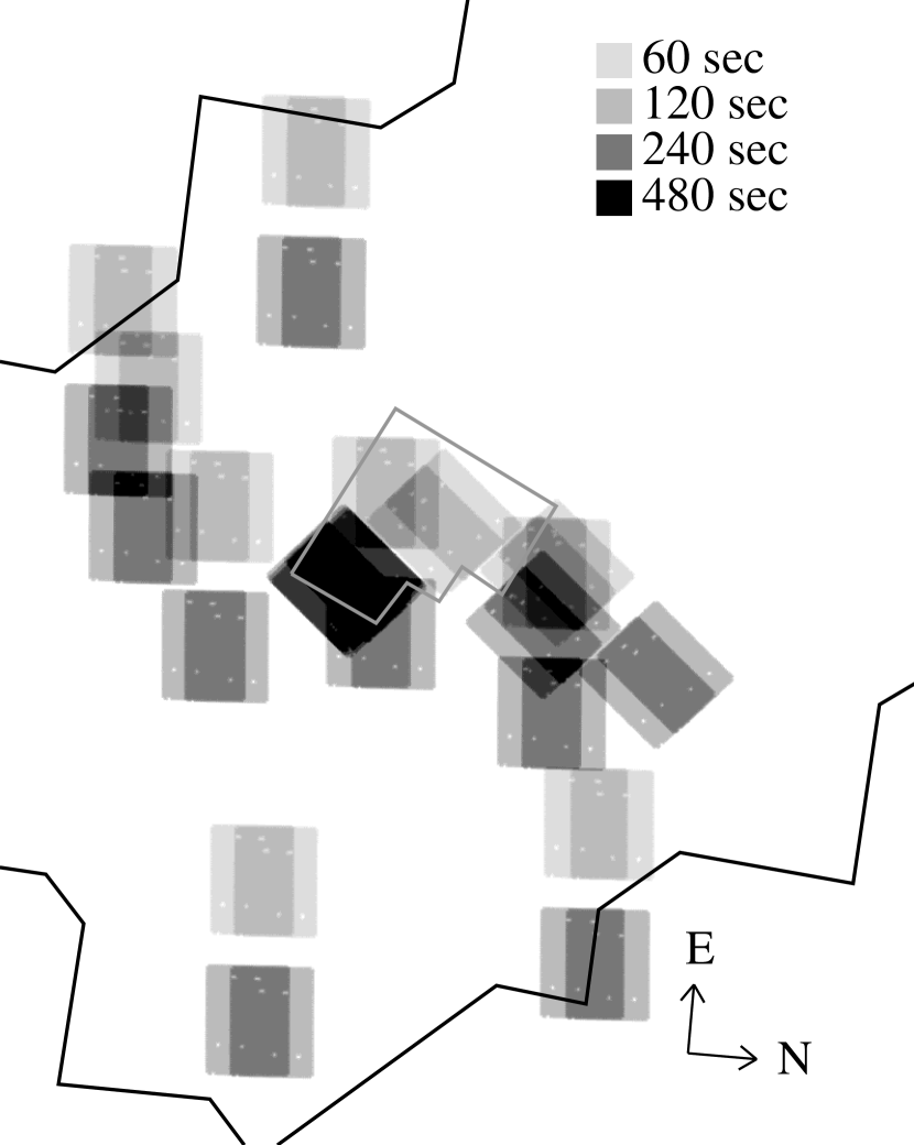
Data were obtained as part of IRS calibration activities during Science Verification (SV) and in parallel with a Guaranteed Time Observation (GTO) program to obtain photometry of submillimeter-selected sources in the field (Charmandaris et al., 2004). The SV observations were motivated to provide a direct comparison of Spitzer IRS 16 $\mu$m imaging of individual targets previously observed by ISOCAM (Aussel et al., 1999). The GTO program targeted seven objects mostly outside the ISOCAM area, but within the GOODS field. In each case the full PUI field of view was imaged for each object at both 16 and 22 $\mu$m. During the 22 $\mu$m imaging, 16 $\mu$m data was obtained in parallel. In total, we obtained 72 exposures, of 60 seconds each, for a survey integration time of 1.2 hours.

While the astronomical observing template (AOT) for “sample up the ramp” (SUR) PeakUp imaging was not commissioned until the second Spitzer proposal cycle (GO2), a work-around was developed using the standard spectroscopic staring-mode AOT. By selecting the short-low (SL) slit and properly offsetting the telescope, PeakUp images were obtained of selected areas around the HDF-N. This technique was used for both the SV and GTO observations, and it resulted in the sparse 16 $\mu$m map shown in Figure 1.

IRS 16$\mu$m images were reduced with the standard pipeline at the Spitzer Science Center (SSC; see chapter 7 of the Spitzer Observer’s Manual). Although pipeline calibrated data have had nominal low-background sky images subtracted, some residual sky signal may remain. We create median sky images from near-in-time subsets of the data, after object masking. We register the sky subtracted images using the MOPEX software provided by SSC. Given the sparseness of objects in the fields, we rely on the reconstructed pointing to provide the registration. The pointing (without the refinement afforded by known stars in the IRAC and MIPS) is typically good to $\sim 1^{\prime\prime}$. The Point Spread Function (PSF) at 16$\mu$m has a full width at half maximum (FWHM) of $\sim 3.6$ arcseconds, compared to the IRAC 8 $\mu$m PSF of 1.98^′′ and the MIPS 24 $\mu$m width of 5.4^′′.

We identify sources and measure photometry with the SSC’s APEX⁸ software, which includes point source fitting to measure the total flux of the source, as well as source deblending. We cross correlate our list of detected sources with the much deeper IRAC Channel 3 (5.8 $\mu$m) image of the field from GOODS (Dickinson et al. 2005; in prep), allowing a maximum of 2^′′ separation. Using the IRAC data ensures that few, if any, spurious objects are included, allowing us to set our detection threshold at a faint level. The faintest IRAC counterpart has a flux of 10 $\mu$Jy. At that flux level, the integrated source counts are $\sim 18$ per square arcminute (Lacy et al., 2005), so the chance of random contamination within our search radius should be less than 6%.

The GOODS 24 $\mu$m data in the HDF-N reach an unprecedented point source sensitivity limit of $<$20 $\mu$Jy (Chary et al. 2005; in prep). More than 3000 sources are detected in 24$\mu$m over the entire field. The IRS 16$\mu$m sources were matched to the 24$\mu$m catalog using a 3$\arcsec$ positional matching threshold. However, more than 90% of the sources (143/149) are matched to within 1$\arcsec$ and the few outliers were inspected by eye. These were found to be attributable to source blending or low signal/noise in the 16$\mu$m image.

The 16 $\mu$m photometric zeropoint was derived from repeated observations of standard stars. The photometry is referenced to a 10K black body spectrum which represents the stellar calibrator. This referencing is the same as the MIPS calibration, but is different than IRAC and ISOCAM, both of which tie their photometric systems to spectra with $\nu f_{\nu}=const$. The color correction between the systems, however, is small ($<3$%). There is a systematic uncertainty due to flux calibration on the order of 6%. The photometric zero point has been verified with comparion of the PUI data to IRS spectra, which are independently calibrated using different standard stars and a different set of templates. In addition, cross calibration between 22 $\mu$m PUI data and MIPS 24 $\mu$m photometry of faint galaxies shows $<10$% residuals for most high significance sources; this difference is within the range attributable to the difference in wavelength coverage.

We estimate a point source sensitivity of 75 $\mu$Jy, $3\sigma$, in 120 seconds. This is somewhat better than numbers previously reported (Houck et al., 2004), and we attribute the difference to improvements in the SSC pipeline, the very low background of the HDF region and the large number of frames available to optimize the sky subtraction.

3 Results

We detect 149 objects, with fluxes ranging from 21 $\mu$Jy to 1.24 mJy. From the literature, 90 of these sources have redshifts (Cohen et al., 2000; Cowie et al., 2004; Wirth et al., 2004), ranging from 0.11 to 2.59. The median redshift is 0.7; only two sources lie at $z>1.5$. All sources have optical counterparts in the GOODS catalog. Table 1 presents the photometry of the detected sources.

There are 100 Chandra sources from the 2 Msec catalog (Alexander et al., 2003) within the surveyed area. Of these, 33 have 16$\mu$m counterparts, comprising 22% of the 16$\mu$m sample. Fadda et al. (2002) find a higher fraction (16 of 42) of Chandra counterparts to ISOCAM sources, but our survey extends to fainter MIR fluxes. The Spitzer survey area also covers 43 radio sources from the 1.4 GHz survey of Richards (2000), 24 of which have 16 $\mu$m counterparts. Of the these, 17 have Chandra detections with 1^′′ of the radio position, and another 5 have Chandra within 2^′′. We defer more discussion of radio sources to future papers, but see Marcillac et al. (2005) for a comparison of these sources with the ISOCAM survey.

We detect 24 objects in common with ISOCAM, including all of the high significance sources from Aussel et al. (1999) that fall in the Spitzer survey area. Eight sources from the less significant ISO sample are not detected by Spitzer. Three ISOCAM sources are resolved into multiple sources by the higher spatial resolution of the PUI mode. In addition, 11 Spitzer sources are not in the Aussel et al. catalog, but fall within the central area of the ISOCAM map. However, 6 of these have fluxes below 0.1 mJy. Several additional sources are undetected at the edges of the ISOCAM area, where the coverage is less deep.

The redshift distribution of the Spitzer and ISOCAM sources are similar. Matching the Aussel et al. ISOCAM source list to the redshift catalog of Cowie et al. (2004) yields 49 objects with spectroscopic redshifts, with a median of $z=0.79$, compared to the Spitzer median of 0.7. The shape of the redshift distributions is nearly identical, with a steep roll off beyond $z\sim 0.8$ and strong detections in the known redshift overdensities at $z\sim 0.45$ and $z\sim 0.8$ (Cohen et al., 2000).

We compare our 16 $\mu$m photometry directly with ISOCAM 15 $\mu$m observations of the same field. Figure 2 shows the object by object flux comparison. We have applied two color correction terms to the Spitzer fluxes. First, there is the small correction for the difference in the photometric system (see above). Secondly, there is a relatively large correction necessary due to the difference in the effective wavelength of the filters. Figure 3 shows the filter transmission for the Spitzer and ISOCAM filters. If we define the effective wavelength following Reach et al. (2005), we find $\lambda_{eff}=15.5$ for the PUI filter. The ISOCAM LW3 photometry uses $\lambda_{eff}=14.3$ A red source (e.g. $f_{\nu}\sim\lambda^{2}$) will have $\sim 15$% more flux at the redder wavelength, so we adopt that as our color correction in the figure. In general, sources agree within the uncertainties, though the Spitzer fluxes may be systematically high by $\sim 10-20$%. This disagreement may be attributable to the difference in the filter bandpasses between IRS and ISOCAM, as prominent features move into and out of the filters at different redshifts. For example, at redshift $z\sim 0.4$, the 9.7 $\mu$m silicate absorption trough will affect the bluer LW3 filter more than the PUI filter. Figure 4 shows the ratio of flux density in the two filters as a function of redshift for a variety of template sources. As can be seen in the figure, a factor of two is not unrealistic, so the difference in individual objects is reasonable. The four brightest objects in Figure 2 are at redshifts 0.41, 0.45, 1.2, and 2.0.

We also compare the differential galaxy-number counts of our survey to those measured by ISO (Figure 5). We use the exposure map to define the area coverage and depth. For this initial comparison, we do not apply an incompleteness correction. The use of the ultradeep IRAC data ensures that there is little contamination from spurious objects. We see general agreement of the counts within the large error bars. It is important to highlight this agreement, because of the use of ISOCAM number counts as a benchmark for comparison to Spitzer surveys. Substantial differences are seen between the first MIPS 24$\mu$m data (Marleau et al., 2004; Papovich et al., 2004) and the ISOCAM data. Spitzer 24 $\mu$m counts appear to peak at fainter fluxes than those measured by ISO at 15 $\mu$m. Gruppioni et al. (2005) attribute this difference to a population of starburst galaxies seen by Spitzer at higher redshifts than those which contribute to the ISO counts. We conclude that the differences reported between 24 $\mu$m and 15 $\mu$m number counts are real and not the result of systematic observatory-based bias. However, we emphasize that our Spitzer counts are derived from the same field as the faint end of the ISO counts, so we do not remove any effects of cosmic variance.

4 Discussion

The mid-infrared detection of sources with known redshifts enables an estimate to be made of their bolometric luminosity. This is possible because of the empirical correlations seen between the mid- and far-infrared luminosities of IRAS detected galaxies in the local Universe (Chary & Elbaz, 2001). To estimate the bolometric correction of galaxies in our sample, we used a sample of 5 local objects with mid-infrared and far-infrared SEDs accurately determined from Spitzer IRS and IRAS. These are: M51 (Kennicutt et al., 2003, from the SINGS legacy project first data release); F00183-7111 (Spoon et al., 2004), UGC5101, Mrk1014, Mrk463 (Armus et al., 2004); and NGC7714 (Brandl et al., 2004). We integrated the mid-infrared spectrum and the IRAS broadband photometry (Soifer et al., 1989) with a dual temperature dust model to obtain a complete SED from 5-1000$\mu$m.

At the redshift of each 16$\mu$m source, we convolved the redshifted template SEDs through the IRS 16$\mu$m and MIPS 24$\mu$m bandpasses. We selected the template whose 16/24 flux ratio was closest to that observed. The selected template was then scaled to match the observed 16 and 24 micron fluxes using weights which are the inverse of the fractional flux uncertainty. The statistical uncertainties associated with this process are directly proportional to the flux uncertainty which is small due to the high S/N of the GOODS 24$\mu$m data. The systematic uncertainties are substantial since they rely on the assumption that high-redshift infrared SEDs are similar to that of local galaxies and the fact that the galaxy SEDs chosen here do not span the whole range of dust templates (see e.g. Chary & Elbaz, 2001, Marcillac et al. 2005, in prep.).

At $z>1.3$, the rest-frame 9.7 $\mu$m silicate absorption feature enters the MIPS 24 $\mu$m wavelength range, and it is likely that varying absorption strength would cause increased scatter in the inferred infrared luminosity ($L_{\mbox{IR}}$). The current sample includes too few objects at that redshift to confirm that expectation.

Figure 6 shows the inferred $L_{\mbox{IR}}$ for the sources in the 16 $\mu$m catalog with spectroscopic redshifts. More than half of the 16 $\mu$m sources (53 of 89) have inferred $L_{\mbox{IR}}$ greater than $>10^{11}~{}L_{\odot}$, implying that they are in the LIRG class, and six of them have ULIRG luminosities. The detection of substantial numbers of sub-LIRG luminosity objects at $z\leq 1$, and sub-ULIRG objects at $z<1.5$, in a few minutes of on-source integration demonstrates the power of the 16 $\mu$m observing mode. We note that the inference of $L_{\mbox{IR}}$ relies on spectroscopic redshifts, which by necessity are biased to the brighter optical sources. Some extremely red, high luminosity sources could be missed. In the particular case of Chandra sources, 75% (25/33) have spectroscopic redshifts, so the bias introduced is likely to be small.

Most of the Chandra-detected sources are among the luminous objects, including three of the six ULIRGs. Two of the ULIRGs are detected in the hard band (2-8 keV), implying at least a contribution from an active nucleus. This result is consistent with existing trends in the literature for ULIRG class objects (Tran et al., 2001). However, we find substantial evidence for AGN activity (and potentially AGN dominated luminosity) below $10^{12}~{}\mbox{L}_{\odot}$.

Because the X-ray data in the 2 Ms field is very deep, not all Chandra sources at these depths are necessarily AGN dominated sources. Fadda et al. (2002) conclude that only 5 of their 16 MIR-detected X-ray sources are unambiguously AGN dominated. In the current sample, we identify 21 hard band (2-8 keV) detections. These galaxies very likely host an AGN, but without a more complete sampling of their SED we cannot definitively determine the AGN contribution to the bolometric luminosity. We examine the ratio of X-ray to infrared luminosities in Figure 7. Alexander et al. (2005) find that most AGN-dominated luminous IR galaxies have ${{L_{X}}\over{L_{\rm FIR}}}>0.004$, but that some AGN sources have ratios as much as ten times lower. They correct the $L_{X}$ for extinction, while we do not; increasing the X-ray flux will only lead to more AGN dominated sources, so our measurement is a lower limit. Alexander et al. also find that sub-millimeter selected sources classified as AGN have photon indices $\Gamma\simeq 1.8$, consistent with local Seyferts. Lower $\Gamma$ values would imply stronger AGN contribution to the X-ray flux. The 16 $\mu$m sources with hard-band Chandra counterparts generally meet one or both of these criteria. The objects most likely to be starbursts (low X-ray to IR ratio and high values of $\Gamma$) are mostly soft-band only sources. The same conclusion is reached using the ratio of infrared to X-ray fluxes, $IR/X$ (Weedman et al. 2004).

The 16 $\mu$m detected X-ray sources have approximately the same distribution of X-ray flux as the non-detections. A marginal difference is seen in their photon indices, with the MIR sample having a median $\Gamma$ value of 1.1 compared to 1.4 for the non-detections. This difference could indicate a higher fraction of AGN in the MIR sample. The same fraction ($\sim 50$%) of each sample has no $\Gamma$ value due either to the faintness of the full-band X-ray flux or to a non-detection in one of the X-ray bands.

4.1 Evidence for PAH emission

The ratio of 16 to 24 $\mu$m flux density is expected to be a strong function of redshift for objects with substantial features in their MIR spectra. These spectra are a combination of: a (usually red) continuum slope; emission from PAH molecules at 6.2, 7.7, 8.6, 11.3, and 12.7 $\mu$m; and a potentially deep silicate absorption trough at 9.7 $\mu$m. Takagi & Pearson (2005) demonstrate the utility of the 16/22 $\mu$m ratio as a crude redshift indicator (the 22 and 24 $\mu$m filters are similar). The relatively broad width of the Spitzer bandpasses complicates the interpretation of the flux ratio, because some redshifts will place both absorption and emission features within the filter.

In Figure 8, we plot the ratio of 16 to 24 $\mu$m flux density, $f_{\nu}$, for the current sample and the expected ratio for local templates, for comparison. We find most sources have flux density ratios of $\sim 0.75$, but that higher ratios are observed at some redshifts. These redshifts are the ones where we expect the redshifting of PAH features to increase the 16 $\mu$m flux density relative to the MIPS 24 $\mu$m flux density. In particular, at redshifts near $z\sim 0.5$, the 11.3 $\mu$m PAH feature is in the middle of IRS 16 $\mu$m band. This feature can have low equivalent width in objects with a strong VSG continuum, such as some ULIRGs, but may dominate in relatively unextinguished starbursts like M51. At redshift $z\sim 0.8$, the 7.7 $\mu$m PAH complex starts to shift into the IRS 16 $\mu$m bandpass, as seen in the rising ratio for M82. At $z\sim 1.3$, two effects contribute to the 16/24 ratio: the silicate absorption feature shifts into the MIPS 24 $\mu$m band, and the 6.2 and 7.7 $\mu$m PAH features are centered in the blue PU bandpass.

It appears that most of the objects in the 16 $\mu$m sample are significantly bluer (that is have higher 16/24 ratios) than the ULIRG template. Despite having high luminosity PAH emission, the ULIRG spectra also have a strong continuum so the PAH’s have low equivalent width (EW) and do not dominate the SED. M51, on the other hand, is dominated by PAH and [NeII] emission. A few sources have even higher 16/24 ratios than M51, which could be explained by a bluer continuum or PAH features with several times higher EWs.

Similar results were observed by Elbaz et al. (2005) and Marcillac et al. (2005) in comparing ISOCAM 15 $\mu$m fluxes to MIPS 24 $\mu$m photometry. They find that the ratio of flux, $\nu f_{\nu}$, for the two filters is consistent with the expected SED for star-forming objects with significant PAH emission. Marcillac et al. examine the ISO HDF-N data, with some sources overlapping the present sample. Their independent measurement also suggests evidence for PAH emission at $z\sim 1$.

We also note that the presence of PAH features helps to distinguish AGN from starburst dominated sources, in sources with weak silicate absorption. Charmandaris et al. (2004) suggest that, in fact, the 16 to 24 $\mu$m flux density ratio can differentiate between the two SED types in the case of SCUBA-selected sources. We find that the present survey shows a low 16/24 ratio for sources with Chandra hard band counterparts. These sources have the ratio expected from the Mrk 231 template. Nonetheless, highly extincted, X-ray weak AGN may still contaminate the starburst portion of the sample. To fully explore this issue, substantial MIR spectroscopic data may be required.

5 Summary and Conclusions

We have presented a pilot study of 16 $\mu$m imaging of faint extragalactic objects with the Spitzer IRS. Our photometric results show good agreement with the 15 $\mu$m ISO survey of the same area. We find evidence of PAH emission at $z\sim 0.5$ and $z>0.8$ in the ratio of 16 to 24 $\mu$m fluxes. The scatter in the flux ratio is large at these redshifts, potentially indicating a broad range of sources with differing emission properties. In principle, we may be able to use photometric surveys such as this one to constrain the strength of the PAH emission relative to the continuum. If so, it may be possible to calibrate the 16 $\mu$m flux as a measurement of star formation at $z\sim 1$. However, such inferences will depend on a good understanding of how the strength of the PAH features varies, as well as a good baseline for the underlying continuum.

These results suggest that larger surveys with the 16 $\mu$m filter will detect PAH emission at $z\sim 1$ in statistically significant samples. The flux limits achievable in a few minutes of observation with the PUI mode will detect sources much fainter than the spectroscopic limit. These observations will enable direct comparison of photometrically measured PAH emission at $z\sim 1$ to those detected at $z\sim 2$ with MIPS.

Table 1: Photometry

R.A. (J2000)	Dec. (J2000)	$f_{16}$ ($\mu$Jy)	$\sigma_{16}$ ($\mu$Jy)	$f_{24}$ ($\mu$Jy)	$\sigma_{24}$ ($\mu$Jy)	$z$	$z$ ref	X-ray ID
189.29108	62.13359	139	24	159	8	$\cdots$	$\cdots$	360
189.23334	62.13561	568	20	832	7	0.792	1	288
189.24095	62.14082	176	19	150	5	0.560	2	$\cdots$
189.22546	62.14306	117	18	258	5	$\cdots$	$\cdots$	281
189.29332	62.14336	236	28	281	8	$\cdots$	$\cdots$	$\cdots$
189.29060	62.14479	878	32	1120	14	$\cdots$	$\cdots$	359
189.25629	62.14495	130	24	185	7	0.703	1	$\cdots$
189.20917	62.14573	348	20	585	8	0.434	1	$\cdots$
189.27412	62.14622	110	16	83	6	$\cdots$	$\cdots$	$\cdots$
189.22844	62.14643	134	17	246	6	0.790	1	$\cdots$
189.30330	62.14756	205	24	273	7	$\cdots$	$\cdots$	$\cdots$
189.18565	62.14861	79	19	98	5	$\cdots$	$\cdots$	$\cdots$
189.29300	62.14959	395	26	407	9	$\cdots$	$\cdots$	$\cdots$
189.19591	62.15186	66	14	90	6	0.905	1	$\cdots$
189.17033	62.15443	99	17	71	5	$\cdots$	$\cdots$	$\cdots$
189.23238	62.15482	408	21	846	10	0.419	1	$\cdots$
189.28125	62.15555	128	24	128	8	$\cdots$	$\cdots$	$\cdots$
189.15843	62.15610	87	27	212	6	0.766	1	$\cdots$
189.18608	62.15747	65	16	47	5	$\cdots$	$\cdots$	$\cdots$
189.19670	62.15831	65	14	53	8	$\cdots$	$\cdots$	$\cdots$
189.20271	62.15891	104	16	127	7	0.517	1	$\cdots$
189.17740	62.15941	343	21	476	6	0.530	1	$\cdots$
189.16095	62.16030	172	25	214	6	0.873	1	$\cdots$
189.17416	62.16194	86	22	117	6	0.845	1	219
189.17314	62.16339	327	23	433	7	0.518	1	217
189.16887	62.16757	89	23	106	6	0.749	1	$\cdots$
189.14030	62.16826	438	25	581	9	1.016	1	177
189.15561	62.17088	78	21	46	5	$\cdots$	$\cdots$	$\cdots$
189.38908	62.17114	197	31	284	10	$\cdots$	$\cdots$	$\cdots$
189.12247	62.17173	158	18	167	5	$\cdots$	$\cdots$	$\cdots$
189.30412	62.17455	102	22	183	6	0.858	1	$\cdots$
189.28342	62.17473	310	22	163	8	$\cdots$	$\cdots$	$\cdots$
189.21304	62.17522	745	29	984	9	0.410	1	265
189.36525	62.17670	878	37	742	8	$\cdots$	$\cdots$	$\cdots$
189.37094	62.17753	226	33	245	6	0.784	1	$\cdots$
189.13484	62.17790	99	18	118	6	$\cdots$	$\cdots$	$\cdots$
189.34918	62.17939	141	24	198	7	0.113	1	$\cdots$
189.12134	62.17940	465	25	724	12	1.013	1	158
189.19768	62.17942	300	29	65	7	$\cdots$	$\cdots$	$\cdots$
189.19420	62.18023	315	29	354	7	0.945	1	$\cdots$
189.13847	62.18055	66	22	51	5	1.006	1	$\cdots$
189.28607	62.18078	193	27	243	6	0.411	1	$\cdots$
189.36378	62.18087	127	27	62	6	$\cdots$	$\cdots$	$\cdots$
189.21376	62.18095	155	30	70	6	$\cdots$	$\cdots$	266
189.30556	62.18172	74	15	114	6	0.936	1	$\cdots$
189.14169	62.18184	115	20	66	5	0.762	1	$\cdots$
189.38663	62.18212	90	21	147	8	$\cdots$	$\cdots$	$\cdots$
189.28464	62.18222	423	26	648	7	0.422	1	353
189.39809	62.18230	488	21	354	7	$\cdots$	$\cdots$	$\cdots$
189.12839	62.18300	88	21	106	6	0.295	1	$\cdots$
189.01353	62.18633	655	33	1210	9	0.639	1	67
189.13100	62.18708	430	20	480	6	1.013	1	$\cdots$
189.38336	62.18852	260	29	235	6	$\cdots$	$\cdots$	$\cdots$
189.17239	62.19147	232	17	287	7	$\cdots$	$\cdots$	$\cdots$
189.32979	62.19196	213	24	190	6	0.556	1	$\cdots$
189.16946	62.19321	68	12	110	5	$\cdots$	$\cdots$	$\cdots$
189.31349	62.19333	96	21	99	5	$\cdots$	$\cdots$	$\cdots$
189.05197	62.19450	973	27	1240	13	0.275	1	$\cdots$
189.01643	62.19463	166	26	69	5	$\cdots$	$\cdots$	$\cdots$
189.02048	62.19480	137	25	59	4	$\cdots$	$\cdots$	$\cdots$
189.19241	62.19494	275	18	290	5	1.011	1	$\cdots$
189.17258	62.19509	134	15	225	5	0.548	1	$\cdots$
189.29378	62.19510	104	23	177	5	0.855	1	$\cdots$
189.03665	62.19544	418	27	265	6	$\cdots$	$\cdots$	$\cdots$
189.17992	62.19660	72	11	113	4	1.009	1	$\cdots$
189.02428	62.19663	109	26	167	4	1.484	2	74
189.15739	62.19703	142	20	173	4	0.838	1	$\cdots$
189.15952	62.19740	189	19	230	3	0.841	1	$\cdots$
188.93968	62.19881	150	21	225	8	$\cdots$	$\cdots$	$\cdots$
189.15422	62.19989	65	17	79	6	0.777	1	$\cdots$
189.02254	62.20059	87	27	71	6	0.456	1	$\cdots$
189.17482	62.20144	74	11	83	5	0.432	1	$\cdots$
189.14368	62.20358	853	32	1290	9	0.456	1	180
189.15337	62.20359	300	22	379	5	0.844	1	$\cdots$
189.16554	62.20385	26	9	28	5	$\cdots$	$\cdots$	$\cdots$
189.17880	62.20448	110	13	114	5	0.454	1	$\cdots$
188.98366	62.20535	295	25	430	6	$\cdots$	$\cdots$	48
189.21553	62.20573	90	19	126	6	0.300	1	267
189.14581	62.20672	315	24	336	6	0.562	1	$\cdots$
189.16486	62.20842	30	9	44	5	$\cdots$	$\cdots$	207
189.15422	62.20854	146	16	232	4	$\cdots$	$\cdots$	$\cdots$
189.20926	62.21098	73	16	119	7	0.474	1	$\cdots$
189.14377	62.21138	923	32	446	5	1.219	1	182
189.15680	62.21138	58	18	70	4	0.457	1	$\cdots$
189.13190	62.21203	95	21	109	5	$\cdots$	$\cdots$	$\cdots$
189.13654	62.21220	141	23	113	6	0.562	1	$\cdots$
189.16635	62.21386	425	20	493	6	0.846	1	211
189.18327	62.21389	343	22	424	5	0.556	1	227
189.17671	62.21447	64	17	26	5	1.240	2	$\cdots$
189.22455	62.21495	207	22	200	6	0.642	1	$\cdots$
189.16197	62.21589	265	22	244	7	1.143	1	203
189.20685	62.21594	66	21	109	6	0.475	1	$\cdots$
189.14230	62.21824	176	24	135	6	$\cdots$	$\cdots$	$\cdots$
189.14310	62.22007	137	26	86	5	0.845	1	$\cdots$
189.20706	62.22025	370	27	371	10	0.475	1	260
189.21022	62.22108	241	30	196	6	0.851	1	$\cdots$
189.14000	62.22213	320	29	323	7	0.843	1	$\cdots$
189.21275	62.22227	118	28	79	6	0.199	1	$\cdots$
189.20445	62.22270	104	32	48	8	$\cdots$	$\cdots$	$\cdots$
189.21581	62.23160	185	30	203	6	0.557	1	$\cdots$
189.19305	62.23459	144	23	211	5	0.961	1	240
189.20628	62.23516	130	20	186	6	0.752	1	258
189.17159	62.23911	60	14	51	6	0.519	1	$\cdots$
189.16225	62.23990	82	17	83	6	$\cdots$	$\cdots$	$\cdots$
189.14830	62.23993	615	32	1480	10	2.005	1	190
189.20126	62.24065	283	20	460	6	$\cdots$	$\cdots$	251
189.12537	62.24105	94	22	183	5	$\cdots$	$\cdots$	$\cdots$
189.14070	62.24189	137	23	188	10	0.519	1	$\cdots$
189.14941	62.24327	179	25	195	15	$\cdots$	$\cdots$	$\cdots$
189.13786	62.24362	107	19	109	6	$\cdots$	$\cdots$	$\cdots$
189.12784	62.24423	71	16	55	6	$\cdots$	$\cdots$	$\cdots$
189.19092	62.24640	79	19	165	7	$\cdots$	$\cdots$	$\cdots$
189.19527	62.24641	193	17	277	11	0.558	1	$\cdots$
189.18340	62.24736	64	15	138	6	$\cdots$	$\cdots$	$\cdots$
189.18481	62.24797	37	16	82	6	1.487	1	229
189.16055	62.24860	75	15	82	6	$\cdots$	$\cdots$	$\cdots$
189.17474	62.24905	80	13	117	6	0.849	2	$\cdots$
189.17014	62.25126	65	15	99	6	$\cdots$	$\cdots$	$\cdots$
189.10291	62.25286	75	17	84	6	0.641	1	$\cdots$
189.13535	62.25359	143	17	142	7	0.684	1	$\cdots$
189.13789	62.25376	41	17	42	7	0.521	1	$\cdots$
189.10132	62.25700	116	23	152	6	0.682	1	$\cdots$
189.16545	62.25726	121	19	161	6	0.380	1	$\cdots$
189.09558	62.25735	335	29	529	6	2.590	1	137
189.19266	62.25759	433	27	544	8	0.851	1	$\cdots$
189.07227	62.25818	448	27	499	7	0.849	1	$\cdots$
188.98537	62.25836	248	24	237	10	$\cdots$	$\cdots$	$\cdots$
189.01689	62.25971	90	20	87	6	$\cdots$	$\cdots$	$\cdots$
188.99142	62.26019	653	35	925	11	$\cdots$	$\cdots$	$\cdots$
189.16722	62.26089	94	20	81	7	$\cdots$	$\cdots$	$\cdots$
189.03229	62.26176	137	24	101	6	$\cdots$	$\cdots$	$\cdots$
189.09373	62.26234	390	28	721	7	0.647	1	132
189.08890	62.26270	210	25	112	5	1.241	2	$\cdots$
189.14543	62.26355	79	17	100	5	0.337	1	$\cdots$
189.00925	62.26373	214	28	176	7	$\cdots$	$\cdots$	62
188.99887	62.26376	1235	34	1470	13	0.375	1	57
189.07265	62.26416	95	23	145	10	0.375	2	$\cdots$
189.01863	62.26440	216	20	102	6	$\cdots$	$\cdots$	$\cdots$
189.03365	62.26478	74	22	125	7	0.459	1	$\cdots$
189.07832	62.26699	176	25	150	5	$\cdots$	$\cdots$	$\cdots$
189.13182	62.26773	245	22	301	5	0.788	1	$\cdots$
189.15320	62.26792	85	17	81	5	0.851	1	$\cdots$
189.12204	62.27040	125	20	208	5	0.847	1	160
189.01381	62.27181	126	18	262	9	$\cdots$	$\cdots$	$\cdots$
189.13525	62.27438	132	18	173	5	0.854	2	$\cdots$
189.14528	62.27447	368	21	482	5	0.847	1	187
189.16695	62.27649	86	22	65	5	$\cdots$	$\cdots$	$\cdots$
189.14203	62.27809	39	17	96	5	$\cdots$	$\cdots$	$\cdots$
189.14694	62.28175	152	17	173	5	$\cdots$	$\cdots$	$\cdots$

Figure 1: (a) The coverage map for the 16 $\mu$m survey. Integration times and position angle are indicated. The central chevron indicates the location of the HDF-N, and the other solid lines denote the limits of the ACS GOODS survey. (b) The cumulative area covered as a function of limiting flux. We show that the majority of the area (30 of 35 square arcminutes) reach a $3\sigma$ sensitiviity of 75 $\mu$Jy or better.

Figure 2: The flux measured with the Spitzer IRS in the 16 $\mu$m bandpass is compared to that measured with ISOCAM in the 15$\mu$m bandpass (LW3) for the objects commonly detected. The diagonal line indicates equal flux. Error bars indicate the 1$\sigma$ uncertainties. Fluxes have been color corrected to the Spitzer photometric system, and for differences between the IRS 16 $\mu$m and ISOCAM LW3 bandpasses (see text).

Figure 3: The filter transmission for the Spitzer blue peak up, 16 $\mu$m, filter (solid line) compared to the ISOCAM LW3, 15 $\mu$m, filter (dotted line). For clarity, both filter curves have been normalized to set their peak transmission to unity.

Figure 4: The predicted ratio of the IRS 16$\mu$m to ISOCAM 15 $\mu$m (LW3) flux densities as a function of redshift based on IRS spectra of template galaxies. We use the extreme silicate-absorption galaxy F00183-7111 (Spoon et al., 2004, solid line), UGC5101, a ULIRG with considerable 9.7$\mu$m absorption (Armus et al., 2004, dashed line), the prototypical AGN Mrk231 (Weedman et al., 2005, dotted line), the typical quasar PG1501+106 from (Hao et al., 2005, tripple-dot-dashed line) and the average mid-IR SED of all starburst galaxies in the IRS GTO program from (Brandl et al., 2005, dot-dashed line).

Figure 5: The differential 16 $\mu$m galaxy number counts measured by Spitzer and ISO. The Euclidean slope has been removed. Poissonian error bars are shown. ISOCAM points include: HDF-N, HDF-S, and the Marano surveys (Elbaz et al., 1999, and the references therein); the gravitational lensing cluster survey (Altieri et al., 1999); ELAIS-S1 (Gruppioni et al., 2002); and the Lockman and Lockman Shallow surveys (Rodighiero et al., 2004).

Figure 6: The inferred $L_{\mbox{IR}}$ as a function of redshift for 16 $\mu$m detected sources. Open stars indicates soft-band-only Chandra detections, and filled stars indicate hard-band detections. All other sources are shown as filled circles. The error in inferred $L_{\mbox{IR}}$ may be dominated by the template fitting, so propagated photometric errors are not shown.

Figure 7: The ratio of X-ray to infrared luminosities vs. the photon index. $L_{\rm IR}$ were calculated as described in the text. $L_{X}$ were calculated using the photon index to extrapolate to the rest-frame full-band (0.5-8 keV). Sources without hard-band detections are shown as lower limits. The vertical dashed line shows the ratio of strong AGN limit of 0.004, and the horizontal line shows the local Seyfert $\Gamma$ ratio of 1.8.

Figure 8: The ratio of 16 to 24 $\mu$m flux density, $f_{\nu}$, as a function of redshift. Star symbols indicate sources with Chandra counterparts, filled stars for hard band detections. Template ratios are shown for a PAH-dominated SED (M51; solid line; SINGS DR1; Kennicutt et al., 2003) , an edge-on starburst (M82; thick line; Förster Schreiber et al., 2001), a ULIRG (U5101; dotted line; Armus et al., 2004), and an AGN (Mrk 231; dashed line; Weedman et al., 2005).

References

- Alexander et al. (2003) Alexander, D. M., et al. 2003, AJ, 126, 539
- Alexander et al. (2005) Alexander, D. M., et al. 2005, ApJ, in press
- Altieri et al. (1999) Altieri, B., et al. 1999, A&A, 343, L65
- Armus et al. (2004) Armus, L., et al. 2004, ApJS, 154, 178
- Aussel et al. (1999) Aussel, H., Cesarsky, C. J., Elbaz, D., & Starck, J. L. 1999, A&A, 342, 313
- Brandl et al. (2004) Brandl, B. R., et al. 2004, ApJS, 154, 188
- Brandl et al. (2005) Brandl, B.R., et al. 2005, ApJ, (submitted)
- Charmandaris et al. (2004) Charmandaris, V., et al. 2004, ApJS, 154, 142
- Chary & Elbaz (2001) Chary, R. & Elbaz, D. 2001, ApJ, 556, 562
- Cohen et al. (2000) Cohen, J. G., Hogg, D. W., Blandford, R., Cowie, L. L., Hu, E., Songaila, A., Shopbell, P., & Richberg, K. 2000, ApJ, 538, 29
- Cowie et al. (2004) Cowie, L. L., Barger, A. J., Hu, E. M., Capak, P., & Songaila, A. 2004, AJ, 127, 3137
- Dickinson et al. (2004) Dickinson, M., et al. 2004, ApJ, 600, L99
- Elbaz et al. (1999) Elbaz, D., et al. 1999, A&A, 351, L37
- Elbaz et al. (2005) Elbaz, D., et al. 2005, A&A, in press
- Fadda et al. (2002) Fadda, D., Flores, H., Hasinger, G., Franceschini, A., Altieri, B., Cesarsky, C. J., Elbaz, D., & Ferrando, P. 2002, A&A, 383, 838
- Fazio et al. (2004) Fazio, G. G., et al. 2004, ApJS, 154, 10
- Förster Schreiber et al. (2001) Förster Schreiber, N. M., Genzel, R., Lutz, D., Kunze, D., & Sternberg, A. 2001, ApJ, 552, 544
- Giavalisco et al. (2004) Giavalisco, M., et al. 2004, ApJ, 600, L93
- Gruppioni et al. (2002) Gruppioni, C., Lari, C., Pozzi, F., Zamorani, G., Franceschini, A., Oliver, S., Rowan-Robinson, M., & Serjeant, S. 2002, MNRAS, 335, 831
- Gruppioni et al. (2005) Gruppioni, C., Pozzi, F., Lari, C., Oliver, S., & Rodighiero, G. 2005, ApJ, 618, L9
- Hao et al. (2005) Hao, L. et al. 2005, ApJ, 625, 75
- Houck et al. (2004) Houck, J. R., et al. 2004, ApJS, 154, 18
- Kennicutt et al. (2003) Kennicutt, R. C., et al. 2003, PASP, 115, 928
- Lacy et al. (2005) Lacy, M., et al. 2005, in press
- Marcillac et al. (2005) Marcillac, D., et al. 2005, submitted
- Marleau et al. (2004) Marleau, F. R., et al. 2004, ApJS, 154, 66
- Papovich et al. (2004) Papovich, C., et al. 2004, ApJS, 154, 70
- Reach et al. (2005) Reach, W. T., et al. 2005, PASP, in press; astro-ph/0507139
- Richards (2000) Richards, E. A. 2000, ApJ, 533, 611
- Rieke et al. (2004) Rieke, G. H., et al. 2004, ApJS, 154, 25
- Rodighiero et al. (2004) Rodighiero, G., Lari, C., Fadda, D., Franceschini, A., Elbaz, D., & Cesarsky, C. 2004, A&A, 427, 773
- Soifer et al. (1989) Soifer, B. T., Boehmer, L., Neugebauer, G., & Sanders, D. B. 1989, AJ, 98, 766
- Spoon et al. (2004) Spoon, H. W. W., et al. 2004, ApJS, 154, 184
- Takagi & Pearson (2005) Takagi, T., & Pearson, C. P. 2005, MNRAS, 357, 165
- Tran et al. (2001) Tran, Q. D., et al. 2001, ApJ, 552, 527
- Weedman et al. (2004) Weedman, D., Charmandaris, V., & Zezas, A. 2004, ApJ, 600, 106
- Weedman et al. (2005) Weedman, D., et al. 2005, ApJ, (submitted)
- Williams et al. (1996) Williams, R. E., et al. 1996, AJ, 112, 1335
- Wirth et al. (2004) Wirth, G. D., et al. 2004, AJ, 127, 3121