Resonant Cyclotron Scattering and Comptonization in Neutron Star Magnetospheres

Abstract

Resonant cyclotron scattering of the surface radiation in the magnetospheres of neutron stars may considerably modify the emergent spectra and impede efforts to constraint neutron star properties. Resonant cyclotron scattering by a non-relativistic warm plasma in an inhomogeneous magnetic field has a number of unusual characteristics: (i) in the limit of high resonant optical depth, the cyclotron resonant layer is half opaque, in sharp contrast to the case of non-resonant scattering. (ii) The transmitted flux is on average Compton up-scattered by $\sim 1+2\beta_{th}$, where $\beta_{th}$ is the typical thermal velocity in units of the velocity of light; the reflected flux has on average the initial frequency. (iii) For both the transmitted and reflected fluxes the dispersion of intensity decreases with increasing optical depth. (iv) The emergent spectrum is appreciably non-Plankian while narrow spectral features produced at the surface may be erased.

We derive semi-analytically modification of the surface Plankian emission due to multiple scattering between the resonant layers and apply the model to anomalous X-ray pulsar 1E 1048.1–5937. Our simple model fits just as well as the “canonical” magnetar spectra model of a blackbody plus power-law.

1 Introduction

The magnetospheres of neutron stars are filled with plasma, with the minimum magnetospheric plasma density being on the order of the Goldreich-Julian density $n_{GJ}={\bf B}\cdot{\bf\Omega}/2\pi ec$ (${\bf B}$ is magnetic field , ${\bf\Omega}$ is angular velocity, $e$ is the elementary charge and $c$ is the velocity of light), Goldreich & Julian (1968). The magnetospheric plasma may efficiently scatter and absorb surface emission through resonant cyclotron scattering. If the plasma density in the magnetosphere equals the minimum Goldreich-Julian density, then resonant scattering is not important in the optical-X-ray range (Mikhailovskii et al. , 1982, Eq. (7)). On the other hand, under certain circumstances the real plasma density in the magnetosphere may exceed this minimum value. In rotationally powered pulsars pair excess on closed field lines can be due to pair creation by high energy photons (e.g.  Wang et al. , 1998). In magnetars (e.g.  Woods & Thompson, 2004), large scale currents flowing in the magnetosphere result in particle densities much larger than the Goldreich-Julian density (Thompson et al. , 2002). In accreting sources (e.g. neutron stars in X-ray binaries or isolated neutron stars accreting from the interstellar medium, ISM) the external plasma may penetrate inside the magnetosphere due to the development of instabilities in the boundary layer (Ghosh et al. , 1977; Arons & Lea, 1980). Finally, the presence of a dense magnetospheric plasma is well established in the case of the binary pulsar PSR J0737-3039B, where the multiplicity factor (the ratio of plasma density to Goldreich-Julian density) was inferred to be $\sim 10^{5}$ (Lyutikov & Thompson, 2005).

The presence of a relatively tenuous plasma may lead to large magnetospheric optical depths for scattering and absorption since in soft X-rays the resonant cyclotron cross-section is five to six orders of magnitude larger than the Thomson cross section, Eq. (6). Due to the large resonant cross-section, the amount of electron-ion plasma that must be suspended in the magnetosphere to produce an optical depth of the order of unity is tiny by astrophysical standards, of the order of $10^{9}$ grams total, Eq. (9). Both the emission patterns and spectral properties of the surface radiation are then modified in the magnetosphere, as photons are scattered and their energies are Doppler-shifted in each scatter.

In this paper we describe salient properties of resonant scattering in neutron star magnetospheres and investigate semi-analytically the influence of scattering on emergent spectra in the non-relativistic limit, when the plasma temperatures are smaller than $mc^{2}/k_{B}$ (where $m$ is the electron mass and $k_{B}$ is Boltzmann’s constant). We employ methods of radiative transfer that were developed for line-driven winds (Chandrasekhar, 1945; Sobolev, 1947) and were previously applied to cyclotron scattering by Zhelezniakov (1996). We adopt a simple one-dimension model for photon propagation (called the Schwarzschild-Schuster method) which allows a clear description of the underlying physics. More involved Monte-Carlo simulations which take into account the full three-dimensional structure of the magnetosphere as well as relativistic effects are underway.

The majority of prior work on resonant cyclotron scattering considered either the atmosphere or the accretion column of neutron stars (Wasserman et al. , 1980; Nagel, 1981; Lamb et al. , 1990; Dermer & Sturner, 1991), in which case the thickness of the plasma column $H$ (centimeters or meters) was assumed to be much smaller than the thickness of the resonant layer (see Section 2) $\Delta r\sim\beta_{th}r$ ($r$ is the distance from the center of the neutron star and $\beta_{th}$ is the thermal velocity in terms of the velocity of light). In this case the transfer of resonant radiation occurs in a quasi-homogeneous magnetic field. Higher up in the magnetosphere $H$ becomes larger than $\Delta r$, so that the effects of the magnetic field ’s inhomogeneity become important. In this case properties of resonant scattering are different from the case of a homogeneous magnetic field and are somewhat counterintuitive. For example, Zhelezniakov (1996) has pointed out that in a strongly inhomogeneous magnetic field in the high optical depth limit resonant layers are semi-opaque. Following up on this work, we investigate spectral properties of the transmitted radiation. We show that if a considerably dense, warm plasma is present in the magnetosphere (so that both the resonant cyclotron optical depth and the frequency Doppler shifts during scattering are non-negligible), then (i) the transmitted spectra are modified, so that thermal surface emission has a resulting non-Plankian spectrum; this effect is most pronounced at optical depths $\sim$ few, while for very large optical depths the spectrum remains nearly Plankian; (ii) transmitted radiation is preferentially Compton up-scattered in frequency, so that the real surface temperature may be smaller than the one inferred from spectral fits; (iii) surface spectral features may be erased; (iv) scattering in the optical and X-ray bands occurs in different regimes due to different polarization properties of normal modes (circularly polarized in optical and linearly polarized in X-rays).

We assume that plasma is tenuous, so that typical frequencies are much larger than the plasma frequency, and the typical wavelength is much larger than the skin depth. The refractive indexes are then close to unity and Debye screening is not important in calculating the scattering probabilities. Collisional processes may also be neglected for the densities and temperatures involved. We also assume that initially radiation is not polarized; this is a considerable simplification since neutron star surface emission is expected to be polarized, especially at magnetar field strengths (Lai & Ho, 2003; Ozel, 2003).

2 Resonant Scatter in the Magnetosphere

2.1 Resonant Layers

If the magnetosphere of a neutron star is populated by warm (non-relativistic) plasma, quasi-thermal radiation coming from the surface of the neutron star may experience strong scattering at the cyclotron resonance, located for a given photon energy at a radius

$$r\sim r_{NS}\left({\hbar eB_{NS}\over\epsilon mc}\right)^{1/3}\sim 8r_{NS}b^{1/3}\left({\epsilon\over 1{\rm keV}}\right)^{-1/3},$$ (1)

where $r_{NS}\sim 10^{6}$ cm is the neutron star radius, $B_{NS}$ is the surface magnetic field, $b=B_{NS}/B_{cr}$, $B_{cr}=4\times 10^{13}$ G is the critical magnetic field, $\hbar$ is Plank constant divided by $2\pi$, $m$ is the electron mass, $\epsilon$ is the energy of a photon. The importance of resonant scattering may be characterized by the resonant optical depth (Mikhailovskii et al. , 1982; Zhelezniakov, 1996)

$$\tau_{res}=\int\sigma_{res}ndl={\pi^{2}e^{2}nr\over mc\omega_{B}}\left|{\partial\ln\omega_{B}\over\partial\ln r}\right|^{-1}(1+\cos^{2}\alpha^{\prime})=\tau_{0}{(1+\cos^{2}\alpha^{\prime})}\mbox{}$$

$$\tau_{0}={\pi^{2}e^{2}nr\over 3mc\omega_{B}},$$ (2)

where $\alpha^{\prime}$ is the angle between the incoming photon and the local magnetic field, $\omega_{B}=eB/mc$ is cyclotron frequency, $\sigma_{res}$ is a resonant cross-section

$$\sigma_{res}={\sigma_{T}\over 4}{(1+\cos^{2}\alpha^{\prime})\omega^{2}\over(\omega-\omega_{B})^{2}+\Gamma^{2}/4},$$ (3)

$\Gamma=4e^{2}\omega_{B}^{2}/3m_{e}c^{3}$ is the natural width of the first cyclotron line, $n$ is the plasma density and we assumed dipolar fields with $\left|{\partial\ln\omega_{B}/\partial\ln r}\right|=3$. The meaning of optical depth $\tau_{0}$ is that only $e^{-\tau_{0}}$ fraction of photons coming from direction $\alpha^{\prime}$ passes through the resonant layer without scattering. This is different from the relative number of photons that passes through the resonant layer after experiencing multiple scattering in the layer.

In the spectral range of interest absorbed photons are almost immediately re-emitted since the synchrotron transition times $\sim 1/\Gamma$ are shorter than the dynamical time $r/c$ for

$$r<\left(\frac{4B_{NS}^{2}e^{4}r_{NS}^{6}}{3c^{6}m^{3}}\right)^{1/5}\sim 7.6\times 10^{8}b^{2/5}\,{\rm cm}$$ (4)

Or, in terms of energy

$$\epsilon>\left(\frac{27c^{13}\hbar^{5}m^{4}}{64B_{NS}e^{7}r_{NS}^{3}}\right)^{1/5}=10^{-3}b^{-1/5}{\rm eV}.$$ (5)

Only microwaves and longer waves suffer true absorption; all the higher energy radiation is scattered.

The resonant optical depth (2) greatly exceeds the non-resonant optical depth for Thomson scattering $\tau_{T}\sim Rn\sigma_{T}$,

$${\tau_{res}\over\tau_{T}}\sim{\pi\over 8}{c\over r_{e}\omega_{B}}\sim 10^{5}\left(\frac{1\ \mathrm{keV}}{\hbar\omega_{B}}\right)10^{5}$$ (6)

where $r_{e}=e^{2}/mc^{2}$ is the classical radius of an electron. Estimating the total Thus, the presence of even a tenuous plasma in the magnetosphere may provide a substantial optical depth to resonant scattering. The corresponding optical depth is

$$\tau_{res}\sim\frac{1}{3}\left(\frac{n}{n_{GJ}}\right)\left(\frac{r}{R_{lc}}\right)$$ (7)

so that minimal magnetospheric density is not sufficient to produce considerable absorption, except near the light cylinder. In order to produce an optical depth of the order of unity the required density is

$$n\sim{3B\over\pi^{2}er}\sim{3b\over\pi^{2}}{mc\over\hbar}{mc^{2}\over e^{2}}{r_{NS}^{3}\over r^{4}}$$ (8)

Estimating the total volume of the scattering material as $V\sim 4\pi r^{3}/3$, the total number of scatterers required is only

$$N\sim{b\over\pi r_{e}\lambda_{C}}{r_{NS}^{3}\over r}\leq 10^{33}b.$$ (9)

If the plasma is electron-ion, then this corresponds to a mass of only $\sim 2\times 10^{9}b$ g.

2.2 Resonant Scattering in an Inhomogeneous Magnetic Field

magnetic field the spatial resonance width is

$$\Delta r\sim{\beta_{th}\over\partial_{r}\ln\omega_{B}|\cos\alpha|}=\beta_{th}L_{B}\sim\beta_{T}r/3$$ (10)

where $L_{B}=-1/\partial_{r}\ln\omega_{B}$ and the last equality assumes a dipole magnetic field.

Depending on whether the thickness of the scattering layer $H$ is larger or smaller than the resonant width $\Delta r=\beta_{th}L_{B}$, the radiation transfer occurs in two different regimes: a weakly inhomogeneous field, $\beta_{th}L_{B}\gg H$ (this is relevant to radiation transfer in photosphere and polar column), and a strongly inhomogeneous field $\beta_{th}L_{B}\ll H$, relevant for radiation transfer in the magnetosphere (Zhelezniakov, 1996). In a weakly inhomogeneous field a resonant photon that has been scattered once and whose frequency has been modified due to the Doppler effect, has a final frequency that typically lies outside of the resonant layer, so that the photon is likely to leave the system. For a continuum spectrum falling on the resonant layer this leads to formation of a narrow absorption line. In a strongly inhomogeneous field, $\Delta r\ll H$, a scattered photon typically remains in resonance and can experience multiple scattering. If a warm plasma, $\beta_{th}\leq 1$, fills a considerable fraction of the magnetosphere, the resonant width is smaller that the thickness of the plasma column, $H\sim r$, by a factor of $\beta_{th}/3$, so that resonant scattering occurs in the limit of a strongly inhomogeneous field. For relativistically hot plasma, $\beta_{th}\sim 1$, the width of the resonance becomes comparable to the inhomogeneity scale and the approach developed in this paper is not valid anymore. Resonant scattering in the relativistic limit has been studied in the context of early models of GRBs and pulsar magnetospheres (e.g.  Lamb et al. , 1990; Brainerd, 1992; Sturner et al. , 1995; Lyubarskii & Petrova, 2000; Gonthier et al. , 2000)

2.3 Polarization in resonance

In neutron star magnetospheres both plasma and quantum effects influence the propagation and wave absorption through polarization of normal modes. Depending on the polarization of normal modes, there are two possible regimes of cyclotron radiation transfer. For weak magnetic field and/or low frequencies, plasma effects dominate over quantum effects. In this case waves propagating along the magnetic field are circularly polarized (if plasma is electron-ion) and in the case of warm plasma, $\beta_{th}\leq 1$, radiation transfer occurs on the extraordinary wave, while cross-sections for scattering of the ordinary wave is smaller by $\beta_{th}^{2}$. Alternatively, in a strong magnetic field and/or for high frequencies, wave polarization is determined by quantum vacuum effects. In this case waves are linearly polarized (for parallel propagation) and both modes are strongly scattered.

In resonance, waves remain linearly polarized (dominated by quantum contributions) if the following condition is satisfied (Zhelezniakov, 1996)

$${\omega_{p}^{2}\over\omega_{B}^{2}\beta_{th}}\ll{1\over 45\pi}{e^{2}\over\hbar c}b^{2}.$$ (11)

Assuming that the optical depth is of the order of unity, $\omega_{p}^{2}\sim\omega_{B}c/r$, dipole geometry and $\beta_{th}=0.3$ we can find the photon energy above which polarization is determined by quantum vacuum corrections

$$\epsilon_{c}=3^{3/4}\left({\pi^{3}c^{19}\hbar^{5}m^{7}\tau^{3}\over e^{7}r_{NS}^{3}\beta_{th}^{3}B_{NS}}\right)^{1/8}=6\,b^{1/8}\tau^{3/8}\left({\beta_{th}\over 0.3}\right)^{-3/8}\,{\rm eV}.$$ (12)

Thus, starting from far UV, quantum vacuum corrections to wave polarization dominate over plasma contributions, so that normal modes are linearly polarized and have similar resonant cross-sections (Thompson et al. , 2002).

3 Radiation transfer

3.1 General relations and Schwarzschild-Schuster method

The photon transfer equation is best derived using covariant formulation (Lindquist, 1966). The invariant transfer equation for photon occupation numbers $n$ is

$$k^{\mu}\partial_{\mu}n=\int Sf_{e}{d^{3}p\over\gamma}$$ (13)

where $S$ represents a collision rate between photons with occupation numbers $n$ and electrons with a distribution function $f$. Integration is over electron momenta $d^{3}p$, $\gamma$ is the electron Lorentz factor, $k^{\mu}$ is the photon four-momentum. We wish to write down the equation of radiative transfer for resonant scattering taking into account only linear terms in $\beta$. This is best done in the frame where the electron is at rest and then transforming to the fluid frame (Hsieh & Speigel, 1976; Blandford & Payne, 1982).

The invariant collision integral is

$$S(\nu,{\bf l};\epsilon,{\bf p})=\nu_{0}\int d\Omega^{\prime}_{0}\left(\left({d\sigma(\nu_{0}^{\prime},{\bf l}^{\prime}_{0}\rightarrow\nu_{0},{\bf l}_{0})\over d\Omega_{0}}\right)\left({\nu_{0}^{\prime}\over\nu_{0}}\right)^{2}\left({d\nu_{0}^{\prime}\over d\nu_{0}}\right)[1+n(\nu_{0},{\bf l}_{0})]n(\nu_{0}^{\prime},{\bf l}^{\prime}_{0})\right.-\mbox{}$$

$$\left.\left({d\sigma(\nu_{0},{\bf l}_{0}\rightarrow\nu_{0}^{\prime},{\bf l}^{\prime}_{0})\over d\Omega_{0}}\right)n(\nu_{0},{\bf l}_{0})(1+n(\nu_{0}^{\prime},{\bf l}^{\prime}_{0})\right)$$ (14)

where prime denotes a scattered photon, and subscript $0$ denotes quantities measured in the electron’s rest frame.

We are interested in terms linear in the thermal velocity of the particles, and thus we neglect recoil effects. In this case $\nu_{0}^{\prime}=\nu_{0}$ and the scattering cross-section is symmetric between the two states:

$$\left({d\sigma(\nu_{0}^{\prime},{\bf l}^{\prime}_{0}\rightarrow\nu_{0}{\bf l}_{0})\over d\Omega_{0}}\right)=\left({d\sigma(\nu_{0},{\bf l}_{0}\rightarrow\nu_{0}^{\prime},{\bf l}^{\prime}_{0})\over d\Omega_{0}}\right)={\pi^{2}e^{2}\over mc}\delta\left(\left\{\begin{array}[]{l}\nu_{0}^{\prime}\\ \nu_{0}\end{array}\right\}-\nu_{B}\right)(1+\mu_{0}^{2})(1+\mu_{0}^{\prime,2})$$ (15)

where $\mu_{0}$ is the cosine of the angle between the photon momentum and the direction of the magnetic field . Neglecting induced process, $n\ll 1$, we find

$$S={\pi^{2}e^{2}\over mc}\nu_{B}\int f_{e}{d^{3}p\over\gamma}\int d\Omega^{\prime}_{0}(1+\mu_{0}^{2})(1+\mu_{0}^{\prime,2})\left(n(\nu_{0}^{\prime},{\bf l}^{\prime}_{0})\delta(\nu_{0}^{\prime}-\nu_{B})-n(\nu_{0},{\bf l}_{0})\delta(\nu_{0}-\nu_{B})\right)$$ (16)

Transforming to the lab frame, $\nu_{0}=\gamma(1-\beta\mu)\nu$ and using

$$n(\nu_{0},{\bf l}^{\prime}_{0})=n(\nu^{\prime},{\bf l}^{\prime})\approx n(\nu,{\bf l}^{\prime})+\left(({\bf l}^{\prime}-{\bf l})\cdot{\bf\beta}\right)\nu\partial_{\nu}n(\nu,{\bf l}^{\prime})$$ (17)

we arrive at

$$k^{\mu}\partial_{\mu}n=\nu_{B}{\pi^{2}e^{2}\over mc}\int f_{e}{d^{3}p\over\gamma}(1+\mu_{0}^{2})\int{d\Omega^{\prime}}(1+\mu_{0}^{\prime,2})\times\mbox{}$$

$$\left(\left(1+\left(({\bf l}^{\prime}-{\bf l})\cdot{\bf\beta}\right)\nu\partial_{\nu}\right)n(\nu^{\prime},\mu^{\prime})\delta(\nu^{\prime}\gamma(1-\beta\mu^{\prime})-\nu_{B})-n(\nu,\mu)\delta(\nu\gamma(1-\beta\mu)-\nu_{B})\right)$$ (18)

where $\mu_{0}$ and $\mu_{0}^{\prime}$ now should be expressed in terms of laboratory frame quantities, $\mu_{0}=(\mu-\beta)/(1-\beta\mu)$ and similarly for $\mu_{0}^{\prime}$. Assuming a non-relativistic one-dimensional electron distribution, $f_{e}=f(p_{\parallel})\delta(p_{\perp})/2\pi p_{\perp}$, $\gamma\sim 1$, and a stationary plasma (so that odd power of $\beta$ average to zero), we find

$$\mu\partial_{x}n={\pi^{2}e^{2}\over mc}\nu_{B}\int f_{e}(\beta)d\beta(1+\mu_{0}^{2})\int{d\Omega^{\prime}}(1+\mu_{0}^{\prime,2})\times\mbox{}$$

$$\left(n(\nu^{\prime},\mu^{\prime})\delta(\nu^{\prime}\gamma(1-\beta\mu^{\prime})-\nu_{B})-n(\nu,\mu)\delta(\nu\gamma(1-\beta\mu)-\nu_{B})\right)$$ (19)

In order to investigate the salient features of resonant radiation transfer, we make a simplifying one-dimensional approximation for photon propagation (this is called the Schwarzschild-Schuster method in radiation transfer). More advanced analytical methods, e.g. , using Gauss formula for numerical quadratures (Chandrasekhar, 1944) lead to complicated equations. [Note that Chandrasekhar (1945) used Gauss method for similar problem of line-driven wind, but neglected aberration effects and kinematic enhancement of cross-section, both linear terms in particle velocity $\beta$.] In the Schwarzschild-Schuster method the integral in the source function is replaced by a sum over forward and backward propagating photons. Eq. (19) is then replaced by a system of two equations for $l=\pm 1$:

$$l\partial_{x}n_{l}={\pi^{2}e^{2}\over 2mc}\nu_{B}\int f_{e}(\beta)d\beta\sum_{l^{\prime}=\pm 1}\left(n(\nu^{\prime},l^{\prime})\delta(\nu^{\prime}\gamma(1-\beta l^{\prime})-\nu_{B})-n(\nu,l)\delta(\nu\gamma(1-\beta l)-\nu_{B})\right)$$ (20)

3.2 Radiative transfer in an inhomogeneous magnetic fields

In an inhomogeneous magnetic field radiation transfer occurs both in real space as photons diffuse through the resonant layer, and in frequency space as their frequencies are Doppler shifted at each scattering. Neglecting the natural line width $\Gamma$, at each scatter there is a conserved quantity, the velocity of the particle

$$\beta={\omega-\omega_{B}\over\omega\cos\alpha}={{\omega}^{\prime}-\omega_{B}\over{\omega}^{\prime}\cos{\alpha}^{\prime}}$$ (21)

Thus, resonant radiation transfer on particles with different velocities occur independently (Zhelezniakov, 1996). This allows a simplification of the problem if we consider $\beta$ instead of $\omega$ as an independent variable. Accordingly, we transform to variables $x-\beta$ by multiplying Eq. (20) by $\delta(\nu(1-\beta\mu)-\nu_{B})$ and integrating over $\nu$:

$$\left(\partial_{x}+{\partial_{r}\ln\nu_{B}}\partial_{\beta}\right)n_{+}={\pi^{2}e^{2}\over 2mc}f_{e}(\beta)\left(n_{-}-n_{+}+\beta(n_{-}+n_{+})\right)\mbox{}$$

$$\left(-\partial_{x}+{\partial_{r}\ln\nu_{B}}\partial_{\beta}\right)n_{-}={\pi^{2}e^{2}\over 2mc}f_{e}(\beta)\left(n_{-}-n_{+}-\beta(n_{-}+n_{+})\right)$$ (22)

where $n_{\pm}=\int d\nu n(\nu)\delta(\nu(1\mp\beta)-\nu_{B})$.

In a weakly inhomogeneous magnetic field we can approximate $\omega_{B}=\omega_{B_{0}}\left(1-x/L_{B}\right)$. After dimensionalizing, $x\rightarrow x/L_{B}$, system (22) becomes

$$\left(\partial_{x}+\partial_{\beta}\right)n_{+}={\tau_{res}\over 2}\left(n_{-}-n_{+}+\beta(n_{-}+n_{+})\right)\mbox{}$$

$$\left(-\partial_{x}+\partial_{\beta}\right)n_{-}={\tau_{res}\over 2}\left(n_{-}-n_{+}-\beta(n_{-}+n_{+})\right)$$ (23)

where $\tau_{res}=L_{B}f_{e}(\beta)\pi^{2}e^{2}/mc$.

System (23) differs from the similar equations of Chandrasekhar (1945) and Zhelezniakov (1996) due to the presence of velocity terms on the right-hand side. These terms come from the kinematic factor $1\pm\beta$ in the collision rate. Since we are interested in the non-relativistic limit $\beta\leq 1$, in what follows we neglect terms with $\beta$ on the right hand side. This allows us to obtain an analytical solution for the transfer function. In appendix A we verify the validity of this approximation using Monte-Carlo simulations. In the limit $\beta\rightarrow 0$ system (23) becomes

$$\left(\partial_{x}+\partial_{\beta}\right)n_{+}={\tau_{res}\over 2}\left(n_{-}-n_{+}\right)\mbox{}$$

$$\left(-\partial_{x}+\partial_{\beta}\right)n_{-}={\tau_{res}\over 2}\left(n_{-}-n_{+}\right)$$ (24)

Resonant optical depth $\tau_{res}$ is generally a function of both $x$ (e.g. through the dependence of the density on $x$) and $\beta$. For simplicity we assume that the density is constant, $\tau_{res}=\tau(\beta)$. Introducing new functions $f$ and $g$ (cf.  Chandrasekhar, 1945)

$$n_{+}=e^{-\int\tau(\beta)d\beta/2}f,\hskip 21.68121ptn_{-}=e^{-\int\tau(\beta)d\beta/2}g$$ (25)

Eq. (24) becomes

$$\left(\partial_{x}+\partial_{\beta}\right)f={\tau_{res}\over 2}g,\hskip 21.68121pt\left(\partial_{x}-\partial_{\beta}\right)g=-{\tau_{res}\over 2}f$$ (26)

Which may be expressed as a second order partial differential equation for $f$ only

$$\left(\partial_{x}^{2}-\partial_{\beta}^{2}\right)f+{\partial_{\beta}\ln\tau_{res}}\left(\partial_{x}+\partial_{\beta}\right)f+{\tau^{2}\over 4}f=0$$ (27)

This equation describes the transfer of resonant cyclotron radiation in a hot plasma in an inhomogeneous magnetic field.

As a simple analytically tractable case we assume that the distribution of particles is a “water-bag”

$$\tau(\beta)=\left\{\begin{array}[]{cl}{\tau_{0}\over 2\beta_{th}},&\mbox{ for $|\beta|<\beta_{th}$}\\ 0,&\mbox{ otherwise.}\end{array}\right.$$ (28)

Eq. (27) then becomes

$$\left(\partial_{x}^{2}-\partial_{\beta}^{2}\right)f+{\tau_{0}^{2}\over 16\beta_{th}^{2}}f=0$$ (29)

Assuming that $\omega_{0}$ is the frequency resonant at $x=0$, $\omega_{0}=\omega_{B_{0}}$, the resonance is given by $\omega=\omega_{B_{0}}(1-\xi)$ and $\omega=\omega_{B_{0}}(1+\eta)$. where $\eta=\beta-x$, $\xi=x+\beta$ are forward and backward propagating characteristics. Changing to variables $\xi,\eta$, Eq. (29) becomes

$$-4\partial_{\xi}\partial_{\eta}f+{\tau_{0}^{2}\over 16\beta_{th}^{2}}f=0$$ (30)

The Green’s function for this equation is

$$G(\xi-\xi_{0},\eta-\eta_{0})=I_{0}\left({\tau_{0}\over 4\beta_{th}}\sqrt{(\xi-\xi_{0})(\eta-\eta_{0})}\right)$$ (31)

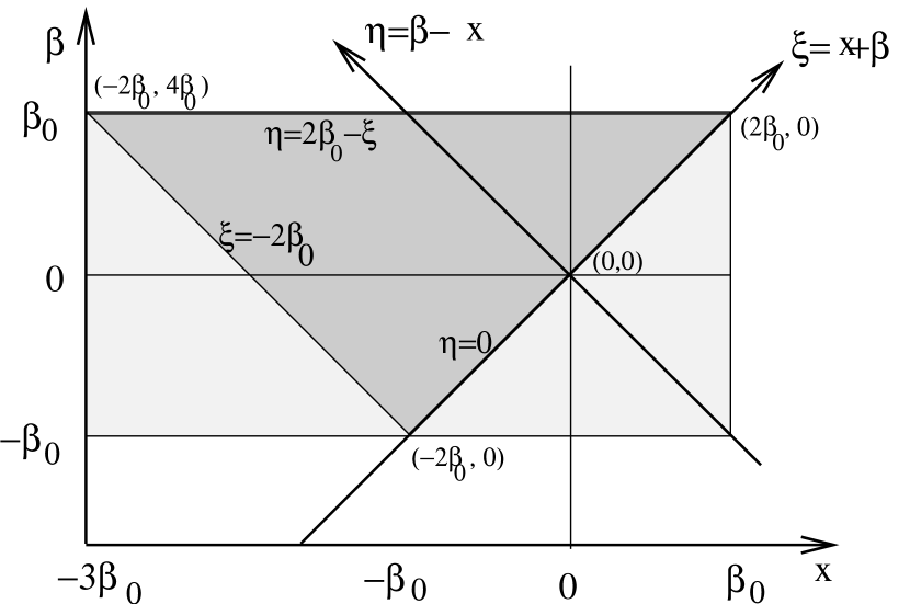
The initial condition for this system is that a monochromatic wave falls onto the inner edge of the resonant layer and that there is no radiation falling on the outer edge. In coordinates $\{\beta,x\}$ the inner boundary of the resonant layer is located at $\beta=-\beta_{th}$, $x=-\beta_{th}$, where $\eta=0$, $\xi=-2\beta_{th}$ (see Fig. 1). At this point we have $n_{+}=\delta(\omega-\omega_{B_{0}})=\delta(\omega_{B_{0}}(x-\beta))=\delta(\eta)/\omega_{B_{0}}$. And $n_{-}=0\propto g\propto\partial_{\xi}f=0$. Thus, the two boundary conditions are

$$f(\xi=-2\beta_{th},\eta)=\delta(\eta)\hskip 21.68121pt\partial_{\xi}f(\xi=-2\beta_{th},\eta)=0$$ (32)

where the intensity has been normalized to unity.

The solution of Eq. (30) given the boundary conditions (32) can be found using standard methods of mathematical physics (e.g.  Courant & Hilbert, 1953).

$$f=\delta(\eta)+{\tau_{0}\over 8\beta_{th}}\sqrt{\xi-\xi_{0}\over\eta-\eta_{0}}I_{1}\left({\tau_{0}\over 4\beta_{th}}\sqrt{(\xi-\xi_{0})(\eta-\eta_{0})}\right)$$ (33)

and

$$n_{+}=e^{-(\eta+\xi+2\beta_{th})\tau_{0}/(8\beta_{th})}\left(\delta(\eta)+{\tau_{0}\over 8\beta_{th}}\sqrt{\xi-\xi_{0}\over\eta-\eta_{0}}I_{1}\left({\tau_{0}\over 4\beta_{th}}\sqrt{(\xi-\xi_{0})(\eta-\eta_{0})}\right)\right)\mbox{}$$

$$n_{-}={\tau\over 8\beta_{th}}e^{-(\eta+\xi+2\beta_{th})\tau_{0}/(8\beta_{th})}I_{0}\left({\tau_{0}\over 4\beta_{th}}\sqrt{(\xi-\xi_{0})(\eta-\eta_{0})}\right)$$ (34)

In the case of a water-bag distribution $\eta_{0}=0$, $\xi_{0}=-2\beta_{th}$, and we find the transmitted and reflected fluxes

$$n_{+}=e^{-\tau_{0}/2}\left(\delta(\eta)+{\tau_{0}\over 8\beta_{th}}\sqrt{4\beta_{th}-\eta\over\eta}I_{1}\left({\tau_{0}\over 4\beta_{th}}\sqrt{\eta(4\beta_{th}-\eta)}\right)\right)\mbox{}$$

$$n_{-}={\tau_{0}\over 4\beta_{th}}e^{-\tau_{0}}I_{0}\left({\tau_{0}\over 4\beta_{th}}\sqrt{(2\beta_{th}-\xi)(\xi+2\beta_{th})}\right)$$ (35)

where the transmitted flux $n_{+}$ should be evaluated at $\xi=2\beta_{th}-\eta$, while the reflected flux $n_{-}$ at $\eta=2\beta_{th}-\xi$. Returning to frequencies $\omega$,

$$n_{+}=e^{-\tau_{0}/2}\left(\delta(\omega-\omega_{0})+{\tau_{0}\over 8\beta_{th}\omega_{0}}\sqrt{\omega_{0}(1+4\beta_{th})-\omega\over\omega-\omega_{0}}I_{1}\left({\tau_{0}\over 4\beta_{th}\omega_{0}}\sqrt{(\omega-\omega_{0})(\omega_{0}(1+4\beta_{th})-\omega)}\right)\right)\mbox{}$$

$$n_{-}={\tau_{0}\over 8\beta_{th}\omega_{0}}e^{-\tau_{0}/2}I_{0}\left({\tau_{0}\over 2\beta_{th}\omega_{0}}\sqrt{\omega_{0}(1+2\beta_{th})-\omega)(\omega-\omega_{0}(1-2\beta_{th}))}\right)$$ (36)

These relations are the solutions for the transfer function, giving the fluxes of transmitted and reflected radiation for an initially monochromatic wave (see Fig. 2).

The reflection probability, found by integrating (36) over frequencies, is

$$p_{refl}=\frac{1-e^{-\tau}}{2}$$ (37)

In the large optical depth limit $p_{refl}=1/2$. (Zhelezniakov, 1996).

For small optical depths

$$n_{+}=\delta(\eta)\left(1-{\tau_{0}\over 4\beta_{th}}(\xi+2\beta_{th})\right)\mbox{}$$

$$n_{-}={\tau_{0}\over 4\beta_{th}}$$ (38)

while in the limit of large optical depths

$$n_{+}={\sqrt{\tau_{0}\over\beta_{th}}\over 4\sqrt{2\pi}\omega_{0}}\left(1+4\beta_{th}-{\omega\over\omega_{0}}\right)^{1/4}\left({\omega\over\omega_{0}}-1\right)^{-3/4}e^{(\omega-\omega_{0}(1+2\beta_{th}))^{2}\tau_{0}/(16\beta_{th}^{2}\omega_{0}^{2})}\mbox{}$$

$$n_{-}={\sqrt{\tau_{0}\over\beta_{th}}\over 4\sqrt{2\pi}\omega_{0}}\left((1+2\beta_{th}-{\omega\over\omega_{0}})({\omega\over\omega_{0}}-(1-2\beta_{th})))\right)^{-1/4}e^{(\omega-\omega_{0})^{2}\tau_{0}/(16\beta_{th}^{2}\omega_{0}^{2})}$$ (39)

3.3 Qualitative properties of resonant transfer function

The properties of the transmitted and reflected fluxes (36) are very different from Thomson scattering and from resonant cyclotron scattering in a homogeneous magnetic field . (Fig. 2). In the small optical depth limit, $\tau_{0}\ll 1$, the reflected wave has an approximately constant spectral flux, $\propto\tau_{0}$, centered at $\omega_{0}$ with dispersion $\Delta\omega/\omega\sim 2\beta_{th}$. The transmitted radiation, $\propto\tau_{0}^{2}$, is up-scattered, spanning $\omega_{0}<\omega<(1+4\beta_{th})\omega_{0}$.

In the large optical depth limit $\tau_{0}\gg 1$ the spectral fluxes of the reflected and the transmitted radiation are equal, so that a resonant layer with high optical depth is half opaque, Eq. (37), see also Zhelezniakov (1996). This is in sharp contrast to the case of non-resonant scattering and to the case of resonant cyclotron scattering in a homogeneous magnetic field , when the transmitted wave is only $\propto e^{-\tau}\ll 1$. Half opaque resonant layers are also reminiscent of the case of line-driven winds (Sobolev, 1947). The transmitted radiation is Compton up-scattered by a factor $\sim 1+2\beta_{th}$, while the reflected waves on average have $\omega\sim\omega_{0}$. Note that this up-scattering is done by a non-relativistic, static warm medium in the limit where recoil effects are neglected, (cf.  Kompaneets, 1956). Next, as optical depth increases, the transmitted and the reflected fluxes have increasingly narrower distributions. The typical dispersion around the central frequency is $\Delta\omega/\omega_{0}\sim 2\sqrt{2}\beta_{th}/\sqrt{\tau}$ for $\tau_{res}\gg 1$. This again can be contrasted with non-resonant Thomson scattering, in which case dispersion increases with increasing $\tau_{res}$.

Consideration of photon residence time inside the resonance layer and number of scattering in the limit of high optical depth also bears a lot of surprises. Residence time inside the layer is independent of optical depth, while number of scattering scales as $\sim\tau_{res}$! To understand this, consider a photon moving outward through a resonant layer. Suppose it is scattered backward at a point $-\beta_{T}<x<\beta_{T}$ on an electron with resonant velocity $\beta=x$ (in dimensionless units). It has already traveled a distance $\beta_{T}+x$ inside a resonance layer. After the scattering the photon energy is $\propto 1+2x$ and the new resonant surface is located at $2x$, so that during scattering the photon is located a distance $\beta_{T}-x$ from the edge of the resonant layer. If it leaves without any further scattering it has traveled a total distance $\beta_{T}+x+\beta_{T}-x=2\beta_{T}$ inside a resonant layer (see Fig. 3). It is easy to see that this quantity does not change at any scattering is valid for any number of scatterings. Thus, regardless of $\tau_{res}$ a photon spends a time $2\beta_{th}r_{res}/c$ in the region where it can resonate with electrons. This can be compared with scaling $\propto\tau$ for residence time and $\propto\tau^{2}$ for number of scattering for non-resonant scattering. An initial short $\delta(t)$-pulse will, of course, be smeared and delayed since depending on scattering history a photon leaves the resonant layer at different spacial coordinates. In the limit of large optical depth spectral smearing is negligible, so that all transmitted photons are delayed by $\beta_{th}r_{res}/c$ with respect to freely propagating ones. (reflected photons are, equivalently, being reflected by a ”wall” located at $r_{res}(1-\beta_{th})$).

The two most unusual characteristics of resonant cyclotron scattering in a strongly inhomogeneous magnetic field are the facts that in the high optical depth limit the transmission coefficient is 1/2 and that the transmitted multiple-scattered photons are preferentially up-shifted in energy (for a water-bag distribution they are always up-shifted in energy). According to (Zhelezniakov, 1996), semitransparence of the resonant layer can be explained in the following way. In the high optical depth limit, most photons will experience the first scatter on electrons moving backwards (along the negative direction $x$) with $\beta\sim-\beta_{th}$. This occurs near the dimensionless coordinate $x\sim-\beta_{th}$. Photons that are re-emitted backwards have their frequency increased by $1+2\beta_{th}$. For these photons the resonant layer is located closer to the star, shifted by $\Delta x=-2\beta_{th}$, so that the reflected photon finds itself outside of the resonant layer. Thus, the photons are trapped between two resonant layers. As a result their escape probability is 1/2 in each direction (see Fig. 3).

To understand the energy up-shift of the transmitted multiple-scattered photons, suppose that a photon is scattered backward at some position $x$ on a particle with velocity $\beta_{1}$. The energy of the photon increases for $\beta_{1}<0$ or decreases for $\beta_{1}>0$. The photon can resonate again only with particles whose velocity satisfies $\beta>\beta_{1}$. As a result, in the subsequent forward scatter its energy will either decrease by an amount smaller than the initial increase (for $\beta_{1}<0$), or increase by an amount larger than the initial decrease (for $\beta_{1}>0$).

3.4 Validity of approximations

For non-relativistic plasma, $\beta_{th}\ll 1$, and for low energy photons, $\epsilon\ll mc^{2}$, recoil frequency shift is small in each scattering event. Since for resonant scattering number of scattering in the limit $\tau_{res}\gg 1$ scales as $\sim\tau_{res}$, the condition for neglect of accumulated recoil is ${\epsilon\over mc^{2}}\tau_{res}\ll\beta_{th}$ where $\epsilon$ is photon energy. For $\sim$ keV photons and $\beta_{th}\sim 0.1$, this limits optical depth to $\tau_{res}\leq 10$. Since in this case the number of scatterings increases with optical depth slower than for non-resonant scattering, this condition on optical depth is less stringent.

For non-relativistic plasma temperatures transition to higher harmonics $s$ are suppressed by $\beta_{th}^{2s}\ll 1$. At high optical depths, $\tau_{0}\gg 1$, such transition may still contribute efficiently to radiation transfer in magnetic field (similar to the case of energy tranfer in wings of highly absorbed lines). The conditions to neglect higher order transition is then $\tau_{0}\beta_{th}^{2s}\ll 1$.

In case of non-resonant scattering, for high optical depth number density of photons increases if compared with the case of no absorption. This leads to increased importance of induced processes. For resonant scattering this is relatively small effect since increase in photon residence time (and corresponding number density) inside the magnetosphere is small, typically a factor $1+\beta_{th}\approx 1$.

4 Magnetar spectra due to resonant scattering

4.1 Magnetospheric plasma in magnetars

In magnetars, large scale currents flow in the magnetosphere, pushed out of the neutron star interior by the slow unwinding of the non-potential magnetic field (Thompson et al. , 2002). The strength of the electrical currents is determined by the speed with which the internal magnetic field unwinds. It is expected that the resulting toroidal magnetic field $B_{\phi}$ is limited by the poloidal field $B_{p}$, $B_{\phi}\leq B_{p}$ (for larger fields the configuration is likely to be unstable to, e.g. , kink modes). If $B_{\phi}\sim\Delta\phi B_{p}$, where $\Delta\phi\leq 1$ is a pitch angle of the magnetic field, the particle density required to carry the current will result in a plasma frequency of the order

$$\omega_{p}^{2}\sim\omega_{B}{c\over v}{c\over r}\Delta\phi$$ (40)

where $v\leq c$ is a the typical velocity the current carries. The resulting optical depth

$$\tau_{res}\sim{c\over v}\Delta\phi$$ (41)

is of the order of unity, regardless of the mass, frequency and magnetic field (Thompson et al. , 2002). Thus, currents flowing in magnetar magnetospheres may provide large optical depth to resonant cyclotron scattering. Electrons then can be heated due to the development of a two stream instability operating on short time scales, $\sim 1/\omega_{p}\sim\sqrt{r/\omega_{B}c\tau}$.

4.2 Multiple scattering of radiation in the X-ray band

Emission from the neutron star’s surface may be modified by resonant scattering. As radiation from the surface propagates in the magnetosphere it is scattered in a resonant layer, some of it is reflected back toward the star and may experience multiple scattering between different hemispheres, so that the emergent spectrum is a sum over many reflections. At every reflection from a resonant layer radiation is broadened by the random motion of resonant electrons, without changing the mean frequency, while the multiply scattered transmitted radiation is Compton up-scattered $1+2\beta_{th}$. If the scattering plasma occupies a large fraction of the magnetosphere, the resulting spectrum is a sum of broadened Plank spectra (the broader the component, the smaller its relative intensity), Compton up-scattered by an optical depth-dependent factor of the order $1+2\beta_{th}$.

First, we calculate semi-analytically the transmitted flux for initially Plankian spectra by summing over multiple reflections between resonant layers located in different hemispheres. In the spirit of our one dimensional approach, we assume that the scattering surfaces are plane parallel. If the spectrum of the surface emission is given by $n_{s}(\omega_{0})$ then the observed spectrum becomes

$$n_{obs}=\int d\omega_{0}n_{+}(\omega,\omega_{0})n_{s}(\omega_{0})+\int d\omega_{1}n_{+}(\omega,\omega_{1})\int n_{-}(\omega_{1},\omega_{0})n_{s}(\omega_{0})d\omega_{0}+\cdots$$ (42)

where the sum is over multiple reflections. Fortunately, the sum quickly converges since each consecutive term is at least two times smaller than the previous one (for numerical computation we limit the sum to 6 terms, which results in an error of the order of $2\%$ at most).

Results of the calculations are presented in Fig. 4. First, the spectrum is overall up-scattered. The initial spectrum is shifted to higher energies, by as much as $1+2\beta_{th}$ in the limit $\tau_{0}\gg 1$ (for smaller optical depths the shift of the emission peak is smaller). As a consequence, the real surface temperature is smaller by as much as a factor $1+2\beta_{th}$ than the one inferred from the Compton up-scattered flux.

Secondly, for optical depth $\tau_{0}\sim 1$ the transmitted spectrum is non-Plankian, see Fig. 5. Modification of the spectra comes both from increased photon dispersion during each reflection as well as from summing contributions from several reflections. Note, that the non-Plankian form of the transmitted spectrum is mostly prominent at $\tau_{0}\sim$ few. In this case the reflected flux becomes comparable to the initial flux. On the other hand, in the limit of large optical depth $\tau_{0}\gg 1$, each reflection does not lead to an increase in the flux dispersion, so that the transmitted flux remains mostly Plankian, but with the peak shifted to larger energies by $1+2\beta_{th}$.

The asymptotic spectrum at frequencies much higher than the initial frequency can be estimated if we assume that each reflection acts as a Gaussian filter with a typical dispersion $\sigma\sim\beta_{th}\omega_{0}\leq\omega_{0}$ and that the reflection probability is $0<p<1/2$. Neglecting the small frequency shift during the final transmission, the resulting flux $F$ is a sum over all reflections

$$F\propto\sum_{n=0}^{\infty}{e^{-{\omega^{2}\over 2(n+1)\sigma^{2}}}p^{n+1}\over\sqrt{2\pi(n+1)}\sigma}.$$ (43)

For $n\gg 1$ we can substitute the sum by an integration and evaluate the integral by the steepest decent method at $n\sim\omega/(\sqrt{2\ln(1/p)}\sigma)$,

$$F\propto{1\over\sqrt{2}\sigma}e^{-\sqrt{2\over\ln(1/p)}{\omega\over\sigma}}$$ (44)

Qualitatively, it takes on average $n\sim\omega/(\beta_{th}\omega_{0})$ scatterings to reach a frequency $\omega\gg\omega_{0}$, but the intensity of radiation is decreased by $p^{n+1}$. Thus, scattering by weakly relativistic warm plasma with $\beta_{th}\leq 1$ produces a non-thermal spectrum with an exponential cut-off at $\omega\sim k_{B}T/(\hbar\beta_{th})$.

4.3 Spectral Fitting

Motivated by the fact that resonant Compton scattering qualitatively reproduces magnetar spectra, we performed a preliminary analysis to verify that it can also do so quantitatively. We decided to fit our model to a 28.8 ks long Chandra X-ray observatory observation of the anomalous X-ray pulsar (AXP) 1E 1048.1–5937. The data were taken with the ACIS detectors (S3 chip) in CC mode. In the literature 1E 1048.1–5937’s spectrum has been characterized by a two-component model consisting of a blackbody of temperature $k_{B}T\sim 0.6$ keV and a power-law tail with spectral index $\Gamma\sim 3$. We chose this source because its spectrum is intermittent between the anomalous X-ray pulsars (AXPs) and the soft-gamma repeaters (SGRs). An analysis of all magnetar spectra will be done in the future.

Given that our model is semi-analytical we created a table of intensities for different values of $\beta_{th}$, $\tau_{res}$ and $k_{B}T$. We developed software to convert this grid into a format that could be read by the X-ray spectral fitting program XSPEC. Using XSPEC the model was folded through the instrumental response and multiplied by a photoelectric absorption model. Only counts between 0.5-1.67 and 1.91-6.7 keV were included in the fits, leaving 281 channels for spectral fitting. The 1.67-1.91 keV region of the spectrum was ignored because of an instrumental feature in the spectrum. For more details on the analysis of this Chandra observation of 1E 1048.1–5937  see (Gavriil et al. , 2005). In our fits $\beta_{th}$ and $\tau_{res}$ were held fixed at predetermined values but we allowed the column density $N_{H}$, the temperature $k_{B}T$ and the normalization to vary freely. We repeated the procedure for different values of $\beta_{th}$ and $\tau_{res}$ until we minimized a $\chi^{2}$ statistic. Even with our course grid in $\beta$ and $\tau_{res}$ we were able to successfully reproduce the observed spectrum. The fit had a reduced $\chi^{2}_{\mathrm{dof}}=1.05$ for $278$ degrees of freedom (dof). We compared our model to a blackbody plus power law model and a double blackbody model. A summary of our spectral fits is given in Table 1.

For comparison we plot the best-fit blackbody plus power law model and the best-fit resonant Compton scattering model for this observation in Figure 7. It is interesting to note that our model fairs just as well as the “canonical” magnetar spectral model of a blackbody plus power-law model (see Table 1). Furthermore, it is interesting to note that all three models listed in Table 1 have the same number of parameters and fit the data well, however, the resonant Compton scattering model has an advantage: it is a single (rather than a double) component model which has a clear physical interpretation within the framework of the magnetar model.

4.4 Secular spectral variations in magnetars

Most magnetar candidates (AXPs and SGRs) show evidence of secular spectral variability (e.g.  Marsden & White, 2001; Woods & Thompson, 2004). In the magnetar model this is readily explained by a variable current flowing in the magnetosphere producing variable optical depth to resonant scattering (Thompson et al. , 2002). Spectral variations in the persistent emission of magnetar candidates have been prominent during active bursting periods. For example, significant spectral evolution was observed during an outburst of AXP 1E 2259.1+586 involving $\sim$80 bursts within a 3 hr observations (Kaspi et al., 2003). More recently a similar, yet much more subtle change was reported by Rea et al.  (2005) in AXP 1RXS 1708–4009. They find that the source’s spectrum has been softening, specifically they find that the photon index increased from $\Gamma\sim 2.4$ to $\sim$2.8. In both cases the correlation between the luminosity and the hardness of the non-thermal component of the source’s spectrum is consistent with the large-scale current bearing magnetosphere model of Thompson et al.  (2002).

5 Other applications

5.1 Smearing of spectral lines

Atmospheres of neutrons stars were expected to produce spectra abundant with spectral features (e.g.  Zavlin & Pavlov, 2002). Though spectral features were observed in some pulsars, their absence in some prominent sources like RX J1856.5–3754 (Drake et al. , 2002), poses a challenge to atmospheric models, (see, e.g. , van Kerkwijk, 2003, for review). Resonant scattering may provide a possible explanation. Let us calculate the effects of cyclotron scattering in a magnetosphere filled with plasma on a narrow spectral feature superimposed on a thermal spectrum. The initial spectrum is taken to be a thermal plus a narrow emission line located at the energy $\epsilon_{line}=5k_{B}T$ with a width $\Delta\epsilon_{line}=0.1k_{B}T$ and total intensity 1/100 of the blackbody (Fig. 6). The emission passes through the magnetosphere with optical depth $\tau_{0}=1$. After multiple reflections the transmitted intensity is virtually indistinguishable from the one obtained from just a thermal spectrum without an emission line. Thus, scattering in the magnetosphere may provide an explanation for the lack of spectral features in neutron star.

5.2 Optical emission

The character of resonant scattering changes for UV and longer wavelengths, when the wave polarization at resonance becomes circular Eq. (12). Consider, for simplicity, the scattering of unpolarized light in a monopole magnetic field in a one-dimensional approximation in the case when normal modes are circularly polarized. For unpolarized light propagating through an electron-ion plasma, half of the intensity (with circular polarization such that electric field of the waves rotates in the same direction as the positive charges) is transfered without scattering, while the other half (with polarization such that the electric field rotates with the electrons) is scattered with the transfer functions calculated in Section 3. In the limit $\tau_{res}\gg 1$ half of the scattered radiation is re-emitted forward, half backward, so that the transmission coefficient is $3/4$ instead of $1/2$ for the case of linearly polarized waves.

In addition, two possibilities exist for multiple scattering of a reflected photon from the opposite hemisphere. If a photon propagates mostly outside the polarization limiting radius, its polarization does not change along the ray, while for propagation inside the polarization limiting radius its polarization evolves adiabatically. These two possibilities result in qualitatively different scattering regimes: if a photon keeps its polarization, then in the simple one-dimensional picture in the opposite hemisphere the electric field of the wave rotates in the opposite direction to that of the local electron so that photon will not experience any more scatterings. On the other hand, if polarization evolves adiabatically, by the time a photon would reach a resonance in the opposite hemisphere it will become virtually unpolarized and thus can be scattered.

Location of polarization limiting radius $r_{lp}$ can be estimated from the condition $\Delta nr_{lp}\sim\lambda$ where $\lambda$ is wavelength and $\Delta n$ is the difference between refractive indexes of the two normal modes. In the relevant regime $\Delta n={2\alpha\over 60\pi}(B/B_{QED})^{2}$ (Heyl & Hernquist, 1997), which gives

$$r_{lp}=\left({bR_{NS}\alpha_{fin}\epsilon\over 60\pi^{2}c\hbar}\right)^{1/5}=5.7\times 10^{7}b^{2/5}\,{\rm cm}$$ (45)

where $\alpha_{fin}$ is fine structure constant. This is typically larger than resonance radius, so that polarization varies adiabatically.

5.3 Young pulsars

The importance of cyclotron scattering in the magnetosphere on the soft X-ray properties of young pulsars has been first pointed out by Wang et al.  (1998), but see also Ruderman (2003). It was suggested that abundant pair creation may occur on closed field lines which would produce a large optical depth to cyclotron scattering. Unfortunately, the model of the cyclotron blanket proposed in the above references is incorrect since it was assumed that in the high optical depth regime most of the emission is reflected back to the star. In fact, resonant up-scattering leads to an increase of the radiation temperature by a factor $\sim 2\beta_{th}\sim 10-20\%$ at most, contrary to what was proposed by Ruderman (2003).

On the other hand, estimates of the effective emitting area based on the observed luminosity and the effective temperature do change due to resonant scattering. Radii of neutron stars are conventionally found from the luminosity and observed temperature, $R_{bb}\sim(L_{X}/4\pi\sigma_{\mathrm{SB}}T^{4})^{1/2}$, where $L_{X}$ is the observed X-ray luminosity, $\sigma_{\mathrm{SB}}$ is Stefan-Boltzmann constant and $T$ is the temperature inferred from the spectral fit. This is called blackbody radius. Resonant scatering changes estimates of both temperature and luminosity and thus changes estimate of neutron star radius. If effects of resonant Comptonization are important, then the surface temperature is lower than the observed one: $T_{s}\sim T_{X}/(1+2a\beta_{th})$, (where $0<a<1$ is a coefficient dependent on the resonant optical depth). On the other hand, the observed luminosity has contributions both from the thermal surface emission and from the energy of the scattering electrons. In case the number of photons is conserved the total luminosity is $L_{X}\sim(1+2a\beta_{th})L_{X,s}$. Thus, the real radius is larger than blackbody radius:

$$R_{NS}\sim(L_{X,s}/4\pi\sigma_{SB}T_{s}^{4})^{1/2}=R_{bb}(1+2a\beta_{th})^{3/2}$$ (46)

This may have important implications for attempts to determine equation of state of neutron stars.

5.4 Accreting neutron stars

For sources accreting through the magnetosphere at a residual rate $\dot{M}$, the optical depth at energy $\epsilon$ is

$$\tau_{res}\sim{\pi e\dot{M}\over\sqrt{r_{res}GM}m_{p}B_{res}}\sim 1\left({\dot{M}\over 10^{-13}M_{\odot}/yr}\right)b^{-7/6}\left({\epsilon\over\mathrm{1keV}}\right)^{17/6}$$ (47)

with $r_{res}$ given by Eq. (1). This accretion rate is larger than the Bondi rate for a neutron star moving at $\sim 100$ km/sec through the ISM, $\dot{M}_{B}\sim 10^{-17}M_{\odot}$/yr, so that isolated neutron stars which are not high energy pulsars or magnetars cannot support dense, hot magnetospheres (cold plasma may be supported by radiation pressure Dermer & Sturner (1991)). On the other hand, the accretion rate (Eq. 47) is considerably smaller than is typically reached in X-ray binaries. It is expected that most of the accreting material is either channeled along the polar magnetic field lines or is flung out by the propeller effect, but even if a small amount of accreting material gets into the bulk of the neutron star’s magnetosphere (e.g. due to development of resistive instabilities in the boundary layer) the resulting resonant cyclotron optical depth can be considerable.

In addition, even in the accretion column, the effects of magnetic field inhomogeneities are non-negligible since the size of the accretion column $H$, which is typically tens of meters, may become comparable to the width of the resonance layer, which for temperatures of $\sim 5$ keV ($\beta_{th}=0.01$) and dipole magnetic field $L_{B}\sim r_{NS}/3$ is $\delta r=\beta_{th}L_{B}\sim 30$ meters. Thus, effects of magnetic field inhomogeneities should introduce corrections of the order of unity to resonant radiative transfer in the accretion column.

6 Discussion

An astrophysically small amount of matter, heated by some external source of energy, may considerably modify the emergent spectra through resonant cyclotron scattering in the magnetospheres of neutron stars and thus impede the effort to understand the structure and composition of neutron stars and their equation of state. The way emission is modified is qualitatively different both from the case of non-resonant Thomson scattering as well as resonant scattering in homogeneous magnetic field .

During resonant Comptonization the number of photons is conserved, while their energy increases by a factor of $\sim 1+2\beta_{th}$. This photon energy increase comes at the expense of the electron energy. Since the minimal charge densities required to produce an optical depth of the order of unity are small (Eq. 9), leptons are efficiently cooled by Comptonization, so that to be in steady state they should be heated by some energy source. The power required is $\sim\beta_{th}L_{X}$ where $L_{X}$ is the observed X-ray luminosity. Depending on the nature of an object heating can be achieved by different sources. In young pulsars this may be achieved by pair production by high energy $\gamma$-ray emission (Wang et al. , 1998). In magnetars, charges are pulled from the surface by inductive electric fields generated due to slow crustal motion (Thompson et al. , 2002). In X-ray binaries residual accretion through the magnetosphere will heat the plasma due to the release of gravitational energy.

Resonant Comptonization by mildly relativistic plasma generically results in soft non-thermal spectra, similar to what is observed in anomalous X-ray pulsars at intermediate energies, $\leq 10$ keV. Non-thermal effects are most prominent for mildly relativistic plasma $\beta_{th}\leq 1$ at intermediate optical depths, $\tau_{res}\sim 1$. On the other hand, at large optical depths, $\tau_{res}\gg 1$ transmitted spectrum is nearly thermal, but shifted to higher frequencies.

An important advantage of the model is that in our case photons are just moved to higher energies, so that one cannot simply extrapolate the data from the X-rays down to longer wavelengths. In the conventional blackbody plus power law fitting procedure one also needs to assume a low energy cut-off to the power law, (cf.  Halpern & Gotthelf, 2005). Such a cutoff is not required in our model.

As a principal application of the model, we have fitted the non-thermal spectrum of AXP 1E 1048.1–5937 and found a quantitatively good agreement. Besides the production of non-thermal spectra in magnetars, resonant scattering may change estimates of the surface temperature while conserving the overall Plankian form of the spectrum (in case of high optical depths), and may explain the lack of surface spectral lines. Variations of magnetospheric plasma parameters may induce spectral changes on time scales much shorter than the evolutionary time scale of neutron stars.

In this paper we addressed the principal issues related to resonant cyclotron transfer, employing a simple one-dimensional model of resonant radiation transfer in the limit of non-relativistic temperatures of scattering particles with a water-bag distribution. More involved three-dimensional Monte-Carlo simulations are in progress. They will extend the current approach to polarized surface emission. The magnetospheric plasma may be relativistically hot, $\beta_{th}\sim 1$, in which case the diffusion of photons both in frequency and in real space is nonlocal and, in addition, scattering on high harmonics becomes important. Also, possible bulk motion of the scattering plasma may lead to the additional effect of bulk Comptonization. Resonant scattering by relativistic electrons has been invoked by Thompson & Beloborodov (2004) to explain the high energy emission from magnetars. Finally, the fact that surface radiation is not blackbody (e.g.  Zavlin & Pavlov, 2002) should also be incorporated. We plan to address some of these issues in a subsequent publication.

Appendix A One-dimensional Monte-Carlo simulation

Analytical results in Section 3 have been obtained in the limit $\beta\rightarrow 0$, neglecting the kinematic enhancement of the scattering rate by a factor $1-\beta$ due to the motion of a particle. To test the validity of this approximation we perform one-dimensional Monte Carlo simulations of the transfer of resonant cyclotron radiation. In the limit $\beta\ll 1$ we can expand frequencies about the initial frequency $(\omega-\omega_{0})/\omega_{0}\ll 1$ and assume $\omega_{B}=\omega_{0}(1-x)$ where $x$ is a dimensionless coordinate (measured in terms of $L_{B}$). Under these circumstances the resonant velocity is $\beta=\pm(x+\omega-\omega_{0})$ and at each scattering the new frequency becomes $\tilde{\omega}=2\omega_{0}(1-x)-\omega$. At each step the probability of scattering backwards is multiplied by a kinematic factor $1-\beta$. Results for the transmission of a spectral line are present in Fig. 8. At intermediate optical depths back scattered photons have on average higher frequencies. This is due to the fact that photons are more likely to encounter backward propagating electrons, whose cross-section is enhanced by $1+\beta$. On the other hand, at high optical depth deviations from analytical results are small. In this limit photons experience multiple scatterings inside the layer so that the relative velocity of the electrons between each scatter is small and the kinematic enhancement is not important.

Table 1: Phase-averaged spectral fits of 1E 1048.1–5937 for various models.

Parameter	Value
Resonant Compton Scattering Model
$N_{H}$ (1022 cm-2)	$0.76\pm 0.16$
$k_{B}T$ (keV)	$0.39\pm 0.05$
$\beta$	0.3 (fixed)
$\tau_{res}$	3 (fixed)
Flux (10-12 ergs cm-2 s-1)	7.61
Unabs Flux (10-12 ergs cm-2 s-1)	8.64
$\chi^{2}$/dof	293/278
Blackbody + Power Law
$N_{H}$ (1022 cm-2)	$1.18\pm 0.04$
$k_{B}T$ (keV)	$0.585\pm 0.012$
$\Gamma$	$3.08\pm 0.10$
Flux (10-12 ergs cm-2 s-1)	$7.91$
Unabs Flux (10-12 ergs cm-2 s-1)	9.56
$\chi^{2}$/dof	274/276
Blackbody + Blackbody
$N_{H}$ (1022 cm-2)	$0.76\pm 0.03$
$k_{B}T_{1}$ (keV)	$0.458\pm 0.030$
$k_{B}T_{2}$ (keV)	$0.843\pm 0.058$
Flux (10-12 ergs cm-2 s-1)	$7.61$
Unabs Flux (10-12 ergs cm-2 s-1)	8.62
$\chi^{2}$/dof	284/276

Figure 1: Region of resonant interaction in $(x,\beta)$ and $(\xi,\eta)$ coordinates ($\eta=\beta-x$, $\xi=x+\beta$) for a water-bag distribution. Monochromatic light with frequency $\omega_{0}$ propagates through the resonance layer centered at $\omega_{B}(x=0)=\omega_{0}$ and is subsequently scattered by particles occupying the lightly shaded area $|\beta|<\beta_{th}$. Resonance transfer occurs in the darkly shaded triangle delimited by the lines $\eta=0$, $\xi=-2\beta_{th}$, $\eta=2\beta_{th}-\xi$.

Figure 2: Transmitted (solid lines) and reflected (dashed lines) fluxes for a water-bag distribution of particles with $\beta_{th}=0.1$ and different optical depths $\tau_{0}$. For small $\tau_{0}\leq 1$ the reflected photons have a homogeneous distribution since the intensity of the initial beam remains approximately constant. The reflected intensity is $\propto\tau_{0}$. The transmitted flux shows an initial $\delta$-function and a double scattering tail $\propto\tau^{2}$, the different panels show that as the optical depth increases the height of the initial $\delta$-function peak decreases, while the intensity of reflected beam increases. In the limit $\tau_{res}\rightarrow\infty$ both the reflected and the transmitted intensities are equal (one half of the initial intensity). For larger optical depth the dispersion of both the reflected and transmitted intensities decrease . In this limit the transmitted photons are Doppler up-shifted on average by $\Delta\omega/\omega=1+2\beta_{th}$, while the reflected photons have on average $\omega\approx\omega_{0}$.

Figure 3: Illustration why photon always spends dimensionless time $2\beta_{th}$ in the resonance region ($2\beta_{th}L_{B}$ in regular units, where $L_{B}$ is the magnetic field inhomogenuity scale) and why resonant layer is semi-opaque in the limit of high optical depth. Initially, resonant surface $\omega_{0}=\omega_{B}$ is located at $x=0$. A photon experiences backward scattering at position $x$ after traveling a distance $\beta_{th}+x$ inside a resonance layer. New resonance layer is centered at $2x$ so that a photon is located a distance $\beta_{th}-x$ from the inner edge of the resonant layer. If it escapes without furher scattering, it would have spent total time $2\beta_{th}$ inside a resonant layer. For $\tau_{0}\gg 1$ an incident photon is scattered at $x\sim-\beta_{th}$ on electrons with $\beta\sim-\beta_{th}$. Half of the photons are then re-emitted forward with $\omega=\omega_{0}$, and half are re-emitted backward with $\omega=\omega_{0}(1+2\beta_{th})$. For backward propagating photons the new resonant surface is located at $x\sim-2\beta_{th}$, so that photons are trapped between resonant layers and escape with approximately equal probability in both directions.

Figure 4: Modification of an initially Plankian spectrum (dashed line) by multiple cyclotron scattering; $\beta_{th}=0.3$ for different values of $\tau_{res}$.

Figure 5: A fit to the transmitted spectrum (solid line) for optical depth $\tau_{0}=3$ and $\beta_{th}=0.3$. Dashed line is the initial Plank spectrum with $T_{0}=1$, Dotted lines are a Plank fit to the transmitted spectrum at the peak of the emission, $T=1.25$ and a residue. The residue is strongly non-thermal.

Figure 6: Effects of resonant scattering on a line in a spectrum. Initial spectrum (dashed line) is Plankian plus an emission line located at $\hbar\omega_{line}=5k_{B}T$, with a width $\Delta\omega_{line}=0.1k_{B}T$ and total intensity 1/100 of the black body. The transmitted intensity (solid line) is barely above the transmitted intensity for the no line case, Fig. 4, (dotted line). The difference between the two (long dashed line) has a complicated profile, but it’s intensity is only $\sim 1\%$.

Figure 7: X-ray Spectrum of the Anomalous X-ray Pulsar 1E 1048.1–5937 as observed by the Chandra observatory. Left: The data fit with our resonant Compton scattering model. See Table 1 for best-fit parameters. Right: Same spectra but fit to a blackbody plus power law. see Table 1 for the best-fit parameters. The dashed and dotted lines represent the individual model components. See text for details on the analysis

Figure 8: Same as Fig. 2 reproduced using one-dimensional Monte-Carlo simulations with $10^{6}$ photons and taking the $1-\beta$ enhancement of the cross-section into account, $\beta_{th}=0.1$. At intermediate optical depths the reflected flux is skewed towards higher frequencies due to the kinematic enhancement of the cross-section. These simulations are done using a one-dimension approximation for constant $L_{B}$.

References

- Arons & Lea (1980) Arons, J. and Lea, S. M., 1980, ApJ, 235, 1016
- Blandford & Payne (1982) Blandford, R. D. and Payne, D. G., 1982, MNRAS, 194, 1033
- Brainerd (1992) Brainerd, J. J., 1992, ApJ, 384, 545
- Burwitz et al. (2001) Burwitz, V., Zavlin, V. E., Neuhäuser, R., Predehl, P., Trümper, J., & Brinkman, A. C. 2001, A&A, 379, L35
- Chandrasekhar (1944) Chandrasekhar, S., 1944, ApJ, 100, 76
- Chandrasekhar (1945) Chandrasekhar, S., 1945, Reviews of Modern Physics, 17, 138
- Chandrasekhar (1960) Chandrasekhar, S., 1960, ”Radiative transfer”, New York: Dover, 1960
- Courant & Hilbert (1953) Courant, R and Hilbert, D, 1953, Methods of mathematical physics, Interscience
- Dermer & Sturner (1991) Dermer, C. D. and Sturner, S. J., 1991, ApJ, 382, L23
- de Vries et al. (2004) de Vries, C. P. and Vink, J. and Méndez, M. and Verbunt, F. , 2004, 415, L31
- Drake et al. (2002) Drake, J. J. et al. 2002, ApJ, 572, 996
- Feroci et al. (2001) Feroci, M. and Hurley, K. and Duncan, R. C. and Thompson, C., 2001, ApJ, 549, 1021
- Gavriil & Kaspi (2004) Gavriil, F. P. and Kaspi, V. M., 2004, ApJ, 609, L67
- Gavriil et al. (2005) Gavriil, F. P., Kaspi, V. M., Woods, P. M., 2005, submitted to ApJ, astro-ph/0507047
- Ghosh et al. (1977) Ghosh, P. and Pethick, C. J. and Lamb, F. K., 1977, ApJ, 217, 578
- Goldreich & Julian (1968) Goldreich, P. & Julian, W.H. 1969, ApJ, 157, 869
- Gonthier et al. (2000) Gonthier, P. L. and Harding, A. K. and Baring, M. G. and Costello, R. M. and Mercer, C. L., 2000, ApJ, 540, 907
- Kaplan et al. (2002) Kaplan, D. L., Kulkarni, S. R., van Kerkwijk, M. H., Marshall, H. L. 2002, ApJ, 570, L79
- Kaspi et al. (2000) Kaspi, V. M., Lackey, J. R., & Chakrabarty, D. 2000, ApJ, 537, L31
- Kaspi & Gavriil (2003) Kaspi, V. M. & Gavriil, F. P. 2003, ApJ, 596, L71
- Kaspi et al. (2003) Kaspi, V. M., Gavriil, F. P., Woods, P. M., Jensen, J. B., Roberts, M. S. E., & Chakrabarty, D. 2003, ApJ, 588, L93
- Kompaneets (1956) Kompaneets, A.S., 1956, Sov. Phys. JETP, 31, 876
- Lamb et al. (1990) Lamb, D. Q. and Wang, J. C. L. and Wasserman, I. M., 1990, ApJ, 363, 670
- Lindquist (1966) Lindquist, R. W., 1966, Ann. Phys.m 37, 487
- Lyubarskii & Petrova (2000) Lyubarskii, Y. E. and Petrova, S. A., 2000, A&A, 355, 406
- Lyutikov & Thompson (2005) Lyutikov, M., Thompson, C., submitted to ApJ, astro-ph/0502333
- Israel et al. (2001) Israel, G. and Oosterbroek, T. and Stella, L. and Campana, S. and Mereghetti, S. and Parmar, A. N., 2001, ApJ, 560, L65
- Haberl (2004a) Haberl, F., 2004, astro-ph/0401075
- Haberl (2004b) Haberl, F. et al. , 2004, astro-ph/0405485
- Halpern & Gotthelf (2005) Halpern, J. P. and Gotthelf, E. V., 2005, ApJ, 618, 874
- Heyl & Hernquist (1997) Heyl, J. S. and Hernquist, L., 1997, Phys. Rev. D, 55, 2449
- Hsieh & Speigel (1976) Hsieh, S. H., Speigel, E.A., 1976, ApJ, 207, 244
- Hulleman et al. (2000) Hulleman, F. and van Kerkwijk, M. H. and Kulkarni, S. R. , 2000, Nature, 408, 689
- Lai & Ho (2003) Lai, D. and Ho, W. C., 2003, Physical Review Letters, 91, 7
- Marsden & White (2001) Marsden, D. & White, N.E. 2001, ApJ, 551, L155
- Mereghetti & Stella (1995) Mereghetti, S., Stella, L., 1995, ApJ, 442, L17
- Mikhailovskii et al. (1982) Mikhailovskii, A. B. and Onishchenko, O. G. and Suramlishvili, G. I. and Sharapov, S. E., 1982, Soviet Astronomy Letters, 8, 369
- Nagel (1981) Nagel, W., 1981, ApJ, 251, 288
- Paerels et al. (2001) Paerels, F. et al. , 2001, A&A, 365, L298
- Ozel (2003) Özel, F., 2003, ApJ, 583, 402
- Rea et al. (2005) Rea, N. and Oosterbroek, T. and Zane, S. and Turolla, R. and Mendez, M. and Israel, G. L. and Stella, L. and Haberl, F., astro-ph/0505400
- Ruderman (2003) Ruderman, M., astro-ph/0310777
- Sobolev (1947) Sobolev V.V., 1947, ”Moving envelopes of stars”, LGU publishing, Leningrad
- Sturner et al. (1995) Sturner, S. J. and Dermer, C. D. and Michel, F. C., 1995, ApJ, 445, 736
- Thompson & Duncan (1993) Thompson, C. & Duncan, R.C. 1993, ApJ, 408, 194 (TD93)
- Thompson & Duncan (1996) Thompson, C. & Duncan, R.C. 1996, ApJ, 473, 322 (TD96)
- Thompson et al. (2002) Thompson, C., Lyutikov, M., Kulkarni, S. R., 2002, ApJ, 574, 332
- Thompson & Beloborodov (2004) Thompson, C., Beloborodov, A.M., astro-ph/0408538
- Wang et al. (1998) Wang, F. Y.-H. and Ruderman, M. and Halpern, J. P. and Zhu, T., 1998, ApJ, 498, 373
- van Kerkwijk (2003) van Kerkwijk, M.H., 2003, in ”Young Neutron Stars and Their Environments”, F. Camilo and B. M. Gaensler, eds, astro-ph/0310389
- Wasserman et al. (1980) Wasserman, I. and Salpeter, E., 1980, ApJ, 241, 1107
- Woods et al. (2001) Woods, P. M. and Kouveliotou, C. and Göğüş, E. and Finger, M. H. and Swank, J. and Smith, D. A. and Hurley, K. and Thompson, C., 2001, ApJ, 552, 748
- Woods (2003) Woods, P. M., 2003, in Pulsars, AXPs, and SGRs Observed with BeppoSAX and other Observatories, Eds. G. Cusumano & T. Mineo, Mem. S. A. It., (Rome: Aracne), 159
- Woods & Thompson (2004) Woods, P. M. and Thompson, C., 2004, astro-ph/0406133
- Woods et al. (2004) Woods, P. M., Kaspi, V. M., Thompson, C., Gavriil, F. P., Marshall, H. L., Chakrabarty, D., Flanagan, K., Heyl, J., & Hernquist, L. 2004, ApJ, 605, 378
- Zavlin & Pavlov (2002) Zavlin, V. E. and Pavlov, G. G., 2002, Neutron Stars, Pulsars, and Supernova Remnants, W. Becker, H. Lesch, and J. Trümper eds, p263
- Zhelezniakov (1996) Zhelezniakov, V. V., 1996, ”Radiation in astrophysical plasmas”, Dordrecht ; Boston : Kluwer, c1996.,
- Zhelezniakov et al. (1996) Zheleznyakov, V. V. and Serber, A. V. and Kuijpers, J. , 1996, A&A, 308, 465