Comparison between methods for the determination of the primary cosmic ray mass composition from the longitudinal profile of atmospheric cascades

Abstract

The determination of the primary cosmic ray mass composition from the longitudinal development of atmospheric cascades is still a debated issue. In this work we discuss several data analysis methods and show that if the entire information contained in the longitudinal profile is exploited, reliable results may be obtained. Among the proposed methods FCC (’Fit of the Cascade Curve’), MTA (’Multiparametric Topological Analysis’) and NNA (’Neural Net Analysis’) with conjugate gradient optimization algorithm give the best accuracy.

, , , , , , ,

1 Introduction

The study of the longitudinal profile of individual atmospheric cascades started in the early eighties with the development of the fluorescent light detection technique implemented for the first time within the framework of the Fly’s Eye experiment [1]. After these pioneering efforts, there has been only one experimental array continuing this type of studies [2] and only recently a new and much more powerful detector has started to collect data: the Fluorescent Detector (FD) of the Pierre Auger Observatory [3]. This instrument will produce a large data flow over the next decades and is therefore calling for new and accurate data analysis procedures capable to fully exploit the large amount of information contained in the FD data.
It is rather surprising, that while there are many methods, both parametric and non-parametric (KNN, Bayesian methods, pattern recognition, neural nets etc.), used to discriminate individual cascades on the basis of ground–based information [4], very little has been done to exploit the amount of information contained in FD data. To our knowledge, in fact, the most popular method developed so far makes use of the depth of the maximum cascade development ($X_{max}$) [5] and derives the observed mean mass composition as a function of the primary energy. Since in experiments which use fluorescent light for the study of the longitudinal development of atmospheric cascades and for the determination of their energy there is a minimum bias in the detection of cascades of different origin, the observed mass composition coincides practically with the primary composition. It has also to be stressed that this approach relies on statistical grounds and therefore does not allow the identification of the primary particle for each individual cascade. Furthermore, even though in the longitudinal profile the $X_{max}$ parameter is the most sensitive to the mass of the primary particle, its sensitivity is still weak. For instance, at a primary energy of 1 EeV (10¹⁸eV) the mean iron induced cascade has $X_{max}$ only (11-12)% lower than for a proton induced one, i.e. a difference which is of the same order of magnitude as the intrinsic fluctuations in $X_{max}$.
As we shall discuss below, such unsatisfactory situation improves drastically if other, seemingly less significant parameters, are taken into account. Among them, we might have: $N_{max}$ - the number of particles (mostly electrons) in the maximum of the cascade, the speed of rise in the particle number etc. For instance, at fixed primary energy, $N_{max}$ is about the same for all cascades, and even though iron induced cascades produce more muons and less energy is carried out by the electrons, the effects on $N_{max}$ are very small. However, due to the lower energy per constituent nucleon in the primary iron nucleus, the cascade development and the rise of the cascade curve are on average faster than for cascades originating from protons. This useful information is neglected when only $N_{max}$ is taken into account. This type of arguments triggered our efforts to find methods which make use of a larger amount of information contained in the cascade curves and which are capable to allow the identification (at least in terms of probabilities) of the cascade origin also for individual showers. Another statistical approach which uses the whole information on the longitudinal profile of the shower for the identification of its origin was developed by Risse M. et al. [6].
In what follows we shall focus on data similar to those expected from the Fluorescent Detector of the Pierre Auger Observatory: namely on the longitudinal profile of each atmospheric cascade, i.e. on the number of charged particle $N_{ch}$ as the function of the atmospheric depth $X$. As it will be shown below, this profile carries more information than $X_{max}$ or $N_{max}$ alone.
We wish to stress that even though the fraction of the hybrid events, in which the information on the shower from the Pierre Auger Surface Array is supplemented by the Fluorescent Detector data, will hardly exceed 10% of the total statistics accumulated by the Surface Array, these events need to be properly handled since they contain the maximum information. In this paper we restrict ourselves to the analysis of the longitudinal development of cascades. Although tailored for possible applications in the context of the Pierre Auger experiment, the methods described below are quite general and may find application in other similar experiments.

2 The simulated data

In what follows, we assume that the primary energy estimates for hybrid events will be accurate at a few percent level. In fact, simulations show that this accuracy for 50% of events improves from 9.5% at 10¹⁸eV to 2.5% at 10²⁰eV [7]. The data set used to implement and test the methods described in the following sections consists of 8000 vertical cascades produced by particles with the fixed energy of 1 EeV, simulated using the CORSIKA program (version 6.004) [8] with the QGSJet98 [9] hadronic interaction model. Simulations were performed at the Lyon Computer Centre. The primary nuclei were $P$, $He$, $O$ and $Fe$, each of them initiating 2000 cascades. The CORSIKA output provides the number of charged particles at atmospheric depths sampled with 5 g cm^-2 intervals.
We clipped the data at a depth of 200 g cm^-2, since the FD detection threshold does not allow to detect the weak signals at the beginning of the cascade development. The maximum atmospheric depth was set at 870 g cm^-2, roughly corresponding to the level of the Pierre Auger Observatory. In Figure 1 we show a subsample of 50 cascades for each primary.

Figure 1: A few examples of the longitudinal development of 1 EeV vertical atmospheric cascades induced by (clockwise from the upper left panel) protons P, helium He, oxygen O and iron Fe nuclei, respectively. Each plot shows 50 typical cascades.

3 Fit of the Cascade Curve (FCC)

Many methods for the determination of the primary mass composition are based on the fit to the distribution of a variable sensitive to the primary mass by a set of simulated distributions obtained for pure primaries and for their weighted combinations. Values of partial amplitudes obtained as a result of such a fit are then used as a measure of the abundance of different nuclei in the observed mass composition, thus giving the mean mass composition without, however, identifying the origin of each individual cascade. The first requirement is to have a large number of experimental cascades in order to build, with sufficient statistical accuracy, mean cascades for different bins of energy and zenith angles and to derive the standard deviations of the particle number at each atmospheric depth (we call it mean trial cascade). The shape of the mean trial cascade reflects the primary mass composition and should be fitted with a properly weighted combination of a few template cascades derived from simulations for different primary nuclei made with a high statistics in order to eliminate the disturbing effect of fluctuations. Any type of fitting algorithm can be used to derive the best fit amplitudes which in turn provide the measure of the abundance of their parent nuclei in the observed cosmic ray flux.

3.1 Input data and procedure

We divided the available statistics of 8000 simulated cascades into two parts, containing 4000 (4$\times$1000) and 4000 (4$\times$1000) cascades respectively. The first part was used for the formation of the mean trial cascade. In order to put ourselves in the worse possible condition (minimum variance) we assumed a uniform primary mass composition where the abundance of each constituent was 0.25 (1000 cascades for each primary nucleus). The standard deviation of the number of particles for the mean trial cascade was obtained by comparing all individual 4000 cascades with their mean.
Other 4x1000 cascades were used to produce the 4 mean constituent cascades, which we call mean test cascades. The fit of the mean trial cascade was then made in the range of atmospheric depths $200\ gcm^{-2}<X<870\ gcm^{-2}$ using the MINUIT code.

Figure 2: Upper part: mean vertical cascade curve ($\Sigma$ - full line) and its standard deviation ($\sigma$ - dashed line) for the uniform primary mass composition at the energy of 1 EeV. The constituent cascade curves weighted by 0.25 for cascades from P, He, O and Fe nuclei are also shown for comparison. Lower part: the best fit abundances of the primary nuclei obtained by the fitting the mean cascade curve with the MINUIT code. Errors of the obtained abundances are smaller than the size of the symbols.

3.2 Results

The mean trial cascade curve and its standard deviation are shown in Figure 2 (upper panel). The constituent cascades taken with the weight of 0.25 are also shown. As it can be seen, differences between contributions of the various constituent nuclei are small, thus making troublesome to derive their abundance accurately, expecially in view of the relatively large fluctuations, both intrinsic for cascades from each constituent nucleus, and due to the difference in the longitudinal development between cascades from different nuclei. Therefore in order to derive an accurate mean mass composition with FCC a large statistics of cascade events must be collected.
The result of the fit of the mean trial cascade with a set of constituent cascades obtained using the MINUIT code is shown in Figure 2 (lower panel) with its parabolic errors. Since we are interested in the mean mass composition we used as input errors in MINUIT not the standard deviations shown in Figure 2, but the errors of the mean cascade, which are 63 times ($\sqrt{(}4000)$) smaller. The profiles of the constituent cascades were assumed to be known precisely. It is apparent from the Figure 2 that MINUIT reconstructs the primary mass composition correctly and make errors of the obtained primary abundances small.

4 Multiparametric Topological Analysis (MTA)

The MTA method [10], when applied to FD data, relies on a topological analysis of correlations between the most significant parameters of the shower development in the atmosphere. In principle this method could be used also with a greater number of parameters, however, in this paper we restrict ourself to the simple case of two parameters only: X_max (the atmospheric depth of the shower maximum) and N_max (the number of charged particles at the depth of X_max). A scatter plot of these two parameters has been built using the $4\times 2000$ showers. Figure 3 shows the scatter plot for proton-only and iron-only induced showers as well as their projected distributions.

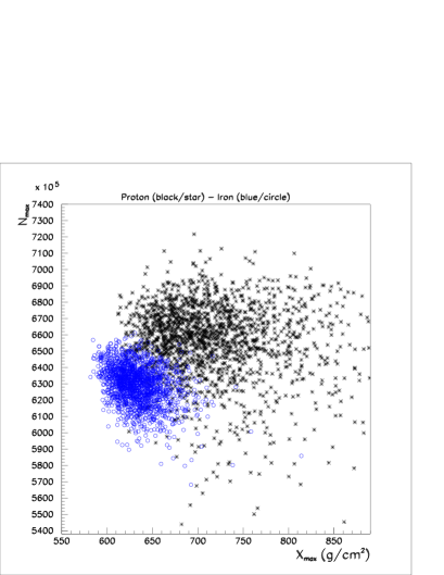
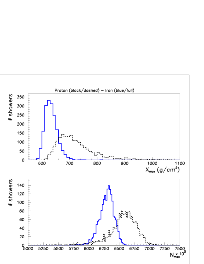
Figure 3: a) N_max vs. X_max scatter plot for proton (star) and iron (circle) induced showers. b) Projected distributions of the scatter plot in Figure 3 for protons (dashed line) and iron nuclei (full line)

It can be seen that the populations arising from the two nuclei are quite well separated in the X_max parameter and less in the N_max parameter. The MTA method consists in dividing the scatter plot in cells whose dimensions are defined by the accuracy with which the parameters can be measured. In our simulations the value of 20 g/cm² has been used as the width of X_max bin, while 5$\times 10^{6}$ was assumed for the width of N_max bin. In each cell we can define the total number of showers N${}_{tot}^{i}$, as the sum of N${}_{P}^{i}$, N${}_{He}^{i}$, N${}_{O}^{i}$ and N${}_{Fe}^{i}$ showers induced by P, He, O and Fe respectively, and then derive the associated frequencies: p${}_{P}^{i}$=N${}_{P}^{i}$/N${}_{tot}^{i}$, p${}_{He}^{i}$=N${}_{He}^{i}$/N${}_{tot}^{i}$, p${}_{O}^{i}$=N${}_{O}^{i}$/N${}_{tot}^{i}$ and p${}_{Fe}^{i}$=N${}_{Fe}^{i}$/N${}_{tot}^{i}$ which can be interpreted as the probability for a real shower falling into the $i^{th}$ cell to be initiated by proton, helium, oxygen or iron primary nuclei. In other words, in the case of an experimental data set of $N_{exp}$ showers, it may be seen as composed by a mixture of N_exp x p_P proton showers, N_exp x p_He helium showers, N_exp x p_O oxygen showers and N_exp x p_Fe iron induced showers, where p${}_{A}=\Sigma^{i}$p${}_{A}^{i}/$N_exp.
In order to generate the $X_{max}-N_{max}$ scatter plot and produce the relevant matrix of cells we used a set of 4$\times$1000 simulated showers. Then we used another subset of 4$\times$600 showers to determine the probabilities $P_{ij}$. For each individual shower $i$ in a given subset the partial probabilities p${}_{P}^{i}$, p${}_{He}^{i}$, p${}_{O}^{i}$ and p${}_{Fe}^{i}$ have been read from the relevant cell i. The sum of such probabilities over the entire subset of 600 showers permits to estimate the probability for a shower of a given nature $A$ to be identified as a shower generated by $P$, $He$, $O$ or $Fe$ primary particle. This probability is shown in Figure 4. One can see that the method attributes the highest probability to the correct nuclei.

Figure 4: Application of the MTA method to the N_max - X_max scatter plot - mean probability $P_{ij}$ for the cascades induced by i nucleus: P, He, O and Fe (specified in headers) being identified as induced by j nucleus, indicated at abscissa .

The application of MTA for the determination of the mean primary mass composition will be described later and compared with the results of other methods.

5 The Minimum Momentum Method (MMM)

Besides various methods of the analysis of the mean mass composition outlined above there is also the possibility to identify the mass of the primary particle for each individual cascade and therefore to determine the observed mass composition. The idea behind this method originated from the well known KNN (’K Nearest Neighbours’) method. In the MMM method [11] as a measure of the closeness between trial (l) and test (m) cascades we decided to use the distance $D_{lm}$, which incorporates all the available information. It takes into account: (i) the longitudinal development of cascades, i.e. the function $N_{ch}(X)$, where $N_{ch}$ is the number of charged particle at the atmospheric depth $X$; (ii) the fluctuations of the cascade development; (iii) the mutual position of the compared cascade curves, i.e. whether the test cascade develops at greater or at lower atmospheric depths with respect to the trial cascade.
This has been achieved by introducing the following definition of distance:

$$D_{lm}=abs[\Sigma_{i}(X_{i}-X^{\ast}_{lm})\frac{N^{l}_{i}-\langle N^{m}_{i}\rangle}{\sigma^{N_{m}}_{i}}]=abs(M_{lm})$$ (1)

Here $N^{l}_{i}$ is the number of charged particles in the trial cascade at the depth of $X_{i}$, $\langle N^{m}_{i}\rangle$ is the number of charged particles at the same depth $X_{i}$ in the mean cascade initiated by the primary nucleus $m$, where $m$ stands for $P,He,O,Fe$. $\sigma^{N_{m}}_{i}$ is the standard deviation of $N^{m}_{i}$ at the depth $X_{i}$ and $M_{lm}$ is the first momentum of the weighted difference. The mean cascades and the standard deviations of their charged particle numbers as a function of the atmospheric depth $X$ are shown in Figure 5.

Figure 5: The mean cascade (full line) and the standard deviation of its particle number (dashed line) for the vertical cascades initiated by primary protons ($P$), helium ($He$), oxygen ($O$) and iron ($Fe$) nuclei (indicated in the upper right corner of the graphs) with the energy of 1 EeV. The abscissa is the atmospheric depth in g cm^-2, the ordinate is the number of charged particles.

Interestingly, the minimum fluctuations is not at the mean depth of the maximum development $X_{max}$ but slightly shifted to the larger depths. This is consequence of the fact that besides the ordinary fluctuations of the particle number there are also fluctuations in the position of the first interaction point ( starting points of the cascade development ). Also remarkable is the fact that the standard deviations do not decrease with increasing primary mass $A$ as $\frac{1}{\sqrt{A}}$ as it is expected for the superposition model. For instance, the fluctuations in iron induced cascades are smaller only by a factor of 2.6 compared with those of proton induced cascades instead of $\sqrt{56}\approx 7.5$. This result confirms the non-validity of the superposition model often used for the estimates.
The fluctuations play an important role since, for instance, in the case of an equal difference in the particle numbers of the trial and mean test cascades, the method favors the mean cascade with the smallest fluctuations.
In order to include the information about the relative location of the trial and the mean test cascade in the atmosphere, we used the term $(X_{i}-X^{\ast}_{lm})$. Here $X^{\ast}_{lm}$ is the depth at which two cascade curves cross (Figure 6).

Figure 6: The Minimum Momentum Method. Panel (a): the trial cascade (left solid line) and the mean test cascades, induced by primary $P$ (right full line), $He$ (dash-dot line), $O$ (dotted line) and $Fe$ (dashed line) nuclei, with which the trial cascade is compared. Panel (b): difference in the particle number between the trial and test cascades. The notations here and in the subsequent graphs are the same as in panel (a). Panel (c): the difference in particle numbers weighted with the standard deviations $\sigma^{N_{m}}_{i}$ shown in Figure 5. Panel (d): the atmospheric depth rescaled with the depth $X^{\ast}_{lm}$ corresponding to the crossing point of the trial and test cascades. Panel (e): the rescaled atmospheric depth multiplied by the weighted difference in the particle number. Panel (f): the first momentum of the weighted difference, obtained just by an integration of the functions shown in panel (e). The minimum of the absolute values of these four momenta defines the origin of the trial cascade (as an example we show an Oxygen nucleus).

In panel $(a)$ of the figure, the trial cascade which is shown by the left solid line, is compared with four test cascades. They are the mean cascades induced by P, He, O and Fe nuclei, as those shown in Figure 5. The difference in the particle numbers between the trial and test cascades is shown in panel $(b)$.
It may be seen that:
(i) the cascades, which are ’to the right’ of the trial cascade ($P$, $He$ and $O$) give a different difference profile with respect to that ’on the left’ ($Fe$);
(ii) the crossing point $X^{\ast}_{lm}$ moves to the left from $P$ to $Fe$.
The weighted difference in particle numbers $\frac{N_{l}-\langle N_{m}\rangle}{\sigma^{N_{m}}_{i}}$ is shown in panel $(c)$. Since all standard deviations are positive, the weighted differences preserve the same sign as the original differences, i.e. they are positive below the crossing point $X^{\ast}_{lm}$ for the ’right’ cascades and negative for the ’left’ ones. Above the crossing point they change sign.
If we simply integrate these curves, the positive and negative parts partly compensate each other and the sensitivity of such integral to the primary mass is reduced. This is why we decided to make the integration for the function which is the product of the weighted difference and the first momentum rescaled to $0$ at the crossing point: $X-X^{\ast}_{lm}$. This rescaled momentum is shown in panel $(d)$. It also changes its sign at the crossing point. When we multiply these functions for ’right’ ($P$, $He$, $O$) cascades the product is negative in the whole range of atmospheric depths, both below and above the crossing point. The same is true for the ’left’ ($Fe$) cascades, but in this case the product is positive. The product functions $(X_{i}-X^{\ast}_{lm})\frac{N^{l}_{i}-\langle N^{m}_{i}\rangle}{\sigma^{N_{m}}_{i}}$ are shown in panel $(e)$. Different signs of the functions for $P$, $He$, $O$ and $Fe$ induced cascades are clearly seen. When we integrate these functions, we obtain the values of the first momentum which have different signs for ’right’ and ’left’ cascades (panel $(f)$). In this way we not only increase the separation between the trial and different test cascades, but we also determine whether the test cascades have earlier or later development in the atmosphere with respect to the trial cascade.
The last problem to be addressed is how to use these momenta for the determination of the parent nucleus. We define it to be the test nucleus which gives the cascade closest to the trial cascade in terms of the distance $(1)$. Therefore we first determine the distances as the absolute value of the momentum $(1)$ and then find their minimum $D_{min}=min(D_{lm})$. The nucleus ${}^{\prime}m^{\prime}$ which gives this minimum is defined as the parent nucleus for the trial cascade. Hence we call this method as the Minimum Momentum Method (MMM).
The probabilities $P_{ij}$ for the cascades induced by primary i nuclei (P, He, O and Fe) being identified as induced by j nuclei are shown in Figure 7. This figure demonstrates that the MMM method works reasonably well in distinguishing light nuclei (P and He) from heavy nuclei (O and Fe), but has not sufficient accuracy to identify separately He and O nuclei.

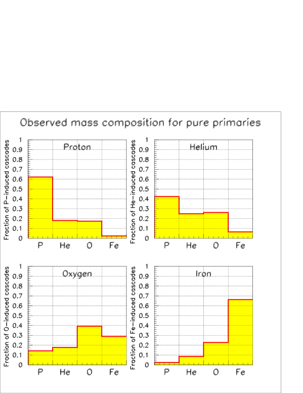
Figure 7: The mean probability for the primary P, He, O and Fe nuclei (specified in the headers of the graphs) to be identified as P, He, O and Fe by MMM. In the MMM each trial $i$ cascade has been associated with just one class of test $j$ cascades.

The application of MMM for the determination of the mean primary mass composition will be described and compared with the results of other methods below.

6 The Neural Net Analysis (NNA)

Neural nets are known to be among the best tools to tackle classification and pattern recognition problems. A Neural Net (hereafter NN) is usually structured into an input layer of neurons, one or more hidden layers and one output layer; neurons belonging to adjacent layers are usually fully connected and the various types and architectures are identified both by the different topologies adopted for the connections as well as by the choice of the activation function. The values of the functions associated with the connections are called “weights” and the whole game of NN’s is in the fact that, in order for the network to yield appropriate outputs for given inputs, the weights must be set to a suitable combination of values [12]. The way this is obtained leads to the first important difference among modes of operations, namely between “supervised” and “unsupervised” methods.
In supervised methods, the network learns by examples and therefore, the user needs to know the correct output value for a fair subsample of the input data. This set needs to be divided into other three subsets named, respectively, Training, Validation and Test (T/V/T) sets. The first subset is used to fine tune the weights, the second one to check whether the network has achieved an acceptable generalization capability and, finally, the third subset is used to evaluate the performances and the classification errors.
In unsupervised methods, instead, input data are clustered on the basis of their statistical properties only. Whether the obtained clusters are or are not significant to a specific problem and which meaning has to be attributed to a given cluster, is not obvious and requires an additional phase called “labeling”. The labeling requires that the user knows the characteristics of a small sample of input vectors (labeled set).
We tested both supervised and unsupervised methods.
The unsupervised experiments were performed using a Self Organizing Map (SOM) [13] with 120 neurons and as labeling set we made use of the same 8000 simulated curves already described. Each neuron was then attributed to a specific class accordingly to the type of event which had activated that neuron more times. Results may be summarised as follows: $P$ = 34% success rate, $He$ = 30%, $O$ = 28%, $Fe$=41%.

Figure 8: Left panel: SOM similarity coloring map: each hexagon represents a neuron and different colors denote different clusters. Right panel: neurons are labeled (A=proton; B=Helium; C=Oxygen; D=Iron).For each neuron the class is determined by the type of nucleus which activetes that neuron the largest number of times

Supervised experiments were instead performed using a Multi Layer Perception (MLP) with Bayesian learning [12] and auxiliary sets extracted from the above quoted simulated curves (for each primary, 1000 input for the training set, 600 and 400 for the validation and test sets respectively). As discussed above, the training set provided the ”a priori” knowledge, the validation set ensured that after training the network still had enough generalization capabilities (thus preventing overfitting, i.e. the fact that the network learns to recognize only the data on which it was trained), the test set is used for evaluating the performance of the network. To be as realistic as possible, i.e., to operate in absence of a priori knowledge as it would be the case for real data, the extraction of the TVT set was made on the basis of the unsupervised clustering which allowed to identify the most significant data subsets and to extract TVT data accordingly. In order for the whole procedure to be effective, all three sets need to be statistically representative of the data to be processed: i.e. they need to sample homogeneously the parameter space. In order to obtain for each input vector the probability that it belongs to a given class, we adopted the SoftMax activation function and the Entropy function as error estimator. Several sets of experiments were performed.

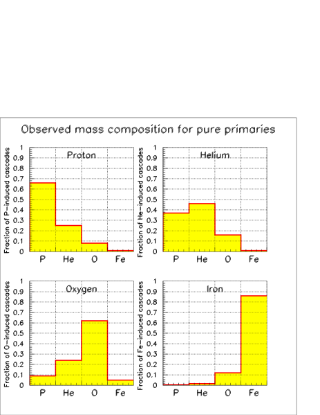
Figure 9: Results for MLP (22 hidden neurons, SoftMax activation function) with conjugate gradient optimization algorithm. The diagrams give the distribution among the four types of primary particles as obtained after labeling.

In a first set of experiments we trained the network on the $6$ parameters resulting from the model driven fit of the Gaisser–Hillas curves and therefore the adopted MLP consisted of $6$ input neurons, one hidden layer with a number of neurons variable from experiment to experiment and $4$ output neurons. Each output neuron corresponds to a class (Proton, Helium, Oxygen, Iron) and provides the probability that the input event belongs to that class. In a second set of experiments we instead trained the net using the entire simulated curve (174 parameters), finding no appreciable difference regardless the adopted NN Architecture - a fact which should not surprise since we are dealing with noiseless data and the best fit curve is a truly good approximation to the data. Results are shown in Figure 9 for the case in which the net had 22 neurons in the hidden layer with conjugate gradient optimization algorithm.
We have used different activation functions (AF) and we have seen they produce quite different results. For instance, the Descendent Gradient AF achieves high accuracy in disentangling the two extreme cases of proton and Iron, but has lower performances for intermediate masses (He and O) which are better separated by the Conjugate Gradient AF [12]. From the above results it is apparent that even in the absence of a fine tuning of the networks, supervised methods outperform unsupervised ones.
It needs to be stressed that, once the network has been trained and frozen, its application to new input data vectors leads to the attribution of the input vector to one and only one of the 4 output neurons, and therefore, each input vector is attributed to one among the four possible classes with an error attached to the individual data point. As in the other methods, however, errors may be estimated as statistical using the test set and the same formalism detailed in the following section. The application of NNA for the determination of the mean primary mass composition and the comparison of its results with results of other methods will be described in the next section.

7 Determination of the primary mass composition

The obtained mean probabilities $P_{ij}$ for the primary mass $i$ to be identified as the mass $j$ in the case of pure primary mass composition can be used for the reconstruction of the mixed primary mass composition as the coefficients in the system of linear equations:

$$n^{\prime}_{P} = n_{P}\cdot P_{P\rightarrow P}+n_{He}\cdot P_{He\rightarrow P}+n_{O}\cdot P_{O\rightarrow P}+n_{Fe}\cdot P_{Fe\rightarrow P}$$

$$n^{\prime}_{He} = n_{P}\cdot P_{P\rightarrow He}+n_{He}\cdot P_{He\rightarrow He}+n_{O}\cdot P_{O\rightarrow He}+n_{Fe}\cdot P_{Fe\rightarrow He}$$ (2)

$$n^{\prime}_{O} = n_{P}\cdot P_{P\rightarrow O}+n_{He}\cdot P_{He\rightarrow O}+n_{He}\cdot P_{O\rightarrow O}+n_{He}\cdot P_{Fe\rightarrow O}$$

$$n^{\prime}_{Fe} = n_{P}\cdot P_{P\rightarrow Fe}+n_{He}\cdot P_{He\rightarrow Fe}+n_{O}\cdot P_{O\rightarrow Fe}+n_{Fe}\cdot P_{Fe\rightarrow Fe}$$

where $n_{P}$, $n_{He}$, $n_{O}$ and $n_{Fe}$ are the true numbers, defining the primary mass composition in the sample $N=n_{P}+n_{He}+n_{O}+n_{Fe}$, which are altered to $n^{\prime}_{P}$, $n^{\prime}_{He}$, $n^{\prime}_{O}$ and $n^{\prime}_{Fe}$, due to a misclassification.
If we define $\Delta_{i}=\frac{n_{i}}{N}$ we can rewrite the system (2) as:

$$\Delta_{j}^{\prime}=\Sigma_{i=1}^{4}P_{ij}\Delta_{i}$$ (3)

where $j=1-4$, $\Delta_{j}^{\prime}$ is the observed abundance of the primary mass $j$, $\Delta_{i}$ is the true abundance of the mass $i$ in the primary cosmic rays with the constraints:

$$\Sigma_{i=1}^{4}\Delta_{i}=\Sigma_{j=1}^{4}\Delta_{j}^{\prime}=1$$ (4)

In order to invert the problem and to reconstruct the abundances $\Delta_{A_{i}}$ in the primary mass composition from the observed abundances $\Delta^{\prime}_{A_{i}}$ and the known probabilities $P_{ij}$, we can apply any method capable to solve the inverse problem taking into account possible errors of the observed distribution with the constraints (4).
In what follows, we use the MINUIT code. The observed abundances were simulated using another subset of 4$\times$400 cascades different from those used for determination of $P_{ij}$. The errors of the observed abundances $\Delta_{A}^{\prime}$ were derived as the errors of the mean for the total number of 1600 cascades. Probabilities $P_{ij}$ were assumed to be known precisely for the MMM and for NNA methods. In this case MINUIT solves the system by the least-square method, i.e. minimizing the function

$$\chi^{2}=\Sigma_{j=1}^{4}\frac{(\Delta_{j}^{\prime}-\Sigma_{i=1}^{4}P_{ij}\Delta_{i})^{2}}{\epsilon_{j}^{2}}$$ (5)

where $\epsilon_{j}$ is the rms error of the difference in the numerator. In the case when probabilities $P_{ij}$ are known precisely this error contains only errors of the observed abundance, i.e. $\epsilon_{j}=\sigma_{n_{j}^{\prime}}$. Due to the constraint (4) we applied rms errors of $\Delta_{j}^{\prime}$, assuming a multinomial distribution of the number of cascades [14]. Actually the multinomial distribution is valid not for the sum of cascades, identified as those induced by nuclei $j$, but separately for each constituent nucleus $i$ identified as $j$, and therefore the error depends on the primary mass composition. The relevant expression for the error in this case is

$$\epsilon_{j}^{2}=\sigma_{\Delta_{j}^{\prime}}^{2}=\frac{\Sigma_{i=1}^{4}\Delta_{i}P_{ij}(1-P_{ij})}{N}$$ (6)

where $N$ is the total number of 4x400 cascades. By this way we introduce a non-linearity into the minimized function $\chi^{2}$, which now becomes a non-linear function of unknown variables $\Delta_{i}$. However, MINUIT is able to solve this problem even in this case.
The results of the solution for the uniform primary mass composition with all abundances $\Delta_{A}=\frac{n_{A}}{N}$ = 0.25 reconstructed by MMM, MTA and NNA methods is shown in Figure 10.

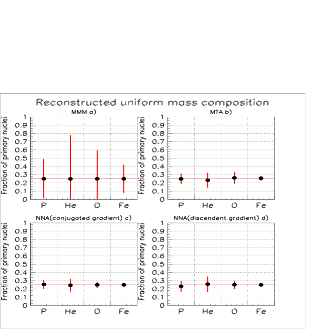
Figure 10: The uniform mass composition ($\Delta_{P}=\Delta_{He}=\Delta_{O}=\Delta_{Fe}=0.25$) reconstructed from the observed mass composition by (a)-MMM, (b)-MTA, (c)-NNA with conjugated gradient optimization algorithm, (d)-NNA with discendent gradient optimization algorithm methods

In the case of MTA it is possible to calculate the errors on the probabilities taking into account that $P_{ij}$ is the mean value of probabilities $P_{ij}^{m}$ in the bins of the grid hit by the cascades $i$, averaged over all these $M$ cascades:

$$P_{ij}=\Sigma_{m=1}^{M}P_{ij}^{m}/M$$ (7)

Since all $P_{ij}^{m}$ are independent of each other, we can write

$$\sigma_{P_{ij}}=\sqrt{\Sigma_{m=1}^{M}\sigma_{P_{ij}^{m}}^{2}}/M$$ (8)

As an example we examine the case when $i=1$ and $j=1,2,3,4$. For $P_{1j}^{m}$ we can write

$$P_{1j}^{m}=\frac{n_{1}^{m}}{\Sigma_{j}^{4}n_{j}^{m}}$$ (9)

or

$$P_{1j}^{m}=\frac{1}{1+\Sigma_{j=2}^{4}(n_{j}^{m}/n_{1}^{m})}$$ (10)

Mind that $n_{j}^{m}$ in the bins are independent of each other. Therefore we can write

$$\sigma_{P_{1j}^{m}}^{2}=(P_{1j}^{m})^{4}\Sigma_{j=2}^{4}\sigma_{(\frac{n_{j}^{m}}{n_{1}^{m}})}^{2}$$ (11)

The distribution of the number of cascades $n_{j}^{m}$ in the bin is also multinomial, but for the large statistics used for the formation of the grid and a small bin size we can approximate it by the Poissonian distribution and write:

$$\sigma_{(\frac{n_{j}^{m}}{n_{1}^{m}})}^{2}=(\frac{n_{j}^{m}}{n_{1}^{m}})^{2}[(\frac{\sigma_{n_{j}^{m}}}{n_{j}^{m}})^{2}+(\frac{\sigma_{n_{1}^{m}}}{n_{1}^{m}})^{2}]=(\frac{n_{j}^{m}}{n_{1}^{m}})^{2}(\frac{1}{n_{j}^{m}}+\frac{1}{n_{1}^{m}})\vskip 6.0pt plus 2.0pt minus 2.0pt$$ (12)

Combining these equations we obtain the errors of the coefficients $P_{1j}$. The same should be done for $i=2,3,4$.
At the end to account for the inaccuracy of $P_{ij}$, in the case of non-zero values of $\sigma_{P_{ij}}$ we suggest to modify the denominator $\epsilon_{j}^{2}$ in the minimized function (5), including these errors into it as

$$\epsilon_{j}^{2}=\sigma_{\Delta_{j}^{\prime}}^{2}+\Sigma_{i=1}^{4}(\sigma_{P_{ij}}\Delta_{i})^{2}=\Sigma_{i=1}^{4}[\frac{\Delta_{i}P_{ij}(1-P_{ij})}{N}+(\sigma_{P_{ij}}\Delta_{i})^{2}]$$ (13)

An additional non-linearity introduced by accounting for these errors $\sigma_{P_{ij}}$, does not prevent MINUIT to find the solution.
The case of uniform primary mass composition taking into account also the errors on the probabilities together a few examples of the non-uniform mass composition in the MTA method are shown in the Figure 11. The errors of the observed abundances $\Delta_{A}^{\prime}$ were derived as the errors of the mean for the total number of 800 cascades (360 for P, 40 for He, 40 for O and 360 for Fe in the first plot of Figure 11, etc.). Comparing Figure 10b and Figure 11a it can be seen that the errors on the probabilities give only a slight change in the errors of mass composition. This is due to the fact the relevant errors come from the ${\Delta_{j}^{\prime}}$ which depend on the statistics.

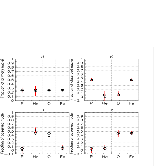
Figure 11: The same as in Figure 10 for MTA method, taking into account the errors of probabilities, in the case of uniform (a) and non-uniform (b,c,d) primary mass composition for three mass compositions. The empty circles are the true abundancies and the full triangles are the reconstructed ones.

8 Discussion

8.1 Comparison of the methods

The comparison of the methods indicates that FCC gives better accuracy in the reconstruction of the mean mass composition than other methods. MTA and NNA give comparable accuracy. In principle MTA could be used also for an individual identification of the cascade origin like MMM by assigning thresholds to the probabilities $P_{ij}$. For example, the cascade i can be associated with primary nucleus j if $P_{ij}$ is the maximum value. It is easy to do if the number of test cascades in the MTA cell is large enough to have a negligible probability for an equal number of test cascades of different groups in the cell. Otherwise there would be many events in which the studied cascade hits a cell with an equal number of test cascades of different groups and an individual identification becomes uncertain.
In the MMM method the achieved mass resolution is not high enough and although the identification is satisfactory for P and Fe, it is not good for He and O. Though MMM uses the whole available information on the cascade profile, it is apparent that the approach which converts all this information into a single distance parameter is not very efficient.
Certainly some other forms of the one-dimensional distance $D_{lm}$ can be proposed for MMM like

$$D_{lm}=\Sigma_{i}[abs\frac{N^{l}_{i}-\langle N^{m}_{i}\rangle}{\sigma^{N_{m}}_{i}}]$$ (14)

or higher odd momenta

$$D_{lm}=abs[\Sigma_{i}(X_{i}-X^{\ast}_{lm})^{n}\frac{N^{l}_{i}-\langle N^{m}_{i}\rangle}{\sigma^{N_{m}}_{i}}]$$ (15)

where $n\geq 3$ should certainly be an odd number in order not to lose the information about the sign of the charged particle difference. However in view of the large overlap between the longitudinal profiles of cascades from different primary nuclei, specifically between P and He, it is unlikely that any approach with a single one-dimensional measure of the distance would give substantially better results.
It is seen in Figure 10 that the NNA method, which does not make a reduction of the available information for the identification of individual cascades gives the better accuracy than MMM.

8.2 Application to experimental cascades

It has to be stressed that all the results outlined above are biased by the fact that we are dealing with the highly unrealistic case of simulated ’noiseless’ data. More realistic testing has to be performed using data which take into account the varying primary energy, and inclination angle, the instrumental signature (noise) and the various sources of errors (uneven and incomplete sampling, etc.). As an example, the 10% error in the energy determination of cascades which have the energy spectrum $\propto E^{-3}$ results in a systematic overestimation of energies about 1%. The corresponding shift of $X_{max}$ is less than 1 $gcm^{-2}$ and is negligible. The shift in $N_{max}$ is more dangerous since the difference between $N_{max}$ for different nuclei is small. The whole 2-dimensional diagram shown in Figure 3a will be displaced down by 60 - 70. This will reduce the abundance of light nuclei and increase the abundance of heavy nuclei. The estimates made ’on the back of envelope’ show that the mean $\langle$ lnA $\rangle$ for the uniform primary mass composition can increase from 2.04 up to 2.20 - 2.25. That is why the use of all the available information for the energy determination including that from the surface detector is of crucial importance.
As for an estimation of uncertainty introduced from different hadronic interaction model, if the real atmospheric cascades develop according to the QGSJET model, but analysed using another model, for example SIBYLL, then since the latter gives cascades slightly displaced towards deeper atmosphere, one can expect the shift of $\langle$ lnA $\rangle$ towards a heavier mass composition of the same magnitude as that caused by an uncertainty of the energy determination.
Coming back to the methods for the determination of the primary mass composition, certainly in order to use FCC the experimentalists should have a set of mean cascade curves and their errors of the mean for test cascades of different energies and zenith angles. Application of MTA and MMM is straightforward - the relevant simulations should be made with a maximum possible statistics. The advantage of MTA is that it is very simple and easy to use. Also there is no problem to extend MTA for larger number of observables - one has just to inrease simulation statistics to create the relevant matrix.
For NNA the problem is more complex since the capability of the neural network to identify particles is strongly related to the possibility to have a realistic T/V/T data sets. Therefore once these sets of data will be available, extensive testing will be performed aimed at selecting the most suitable neural model (in terms of architecture, number of input neurons and hidden layers, activation and error function etc.). One advantage of NNs is that they may be optimized to work on well defined bins of the input parameter space. The use of unsupervised NNs may also be of some help in reducing the dimensionality of the parameter space.
Final goal of the efforts is to implement an optimal classifier (Hyerarchical neural net or something else) capable to combine the classification of all methods tested so far.

9 Conclusions

We proposed and tested four methods for the determination of the primary cosmic ray mass composition in the EeV energy region on the basis of measurements of their longitudinal development: two of them (FCC and MTA) are able to derive the mean mass composition and the other two (MMM and NNA) are based on the identification of the primary mass for each individual cascade. However we stress that this classification depends essencially on the way to derive the probabilities (except for FCC that can be really used only to derive mean mass composition). In fact for MTA we can assign a threshold to the probabilities to associate each event with just one primary particle. On the contrary, for MMM and NNA it can be possible to integrate over all showers to derive the mean mass composition. Among the proposed methods FCC (’Fit of the Cascade Curve’), MTA (’Multiparametric Topological Analysis’) and NNA (’Neural Net Analysis’) with conjugate gradient optimization algorithm give the best accuracy. All methods employ more information about the longitudinal development of atmospheric cascades than just the depth of the cascade maximum. They are independent and can be used complementary for the cross-check of final results.

Acknowledgements

Authors thank Dr.M.Risse for the high statistics simulation of cascades used in this work and remarks on the paper and also Prof. K.-H.Kampert, Prof. H.Rebel, Dr. L.Perrone and Dr. V.P.Pavluchenko for remarks and useful discussions. One of the authors (ADE) thanks INFN, Sezione di Napoli and the University of Catania for providing the financial support for this work and the hospitality.

References

- [1] Baltrusaitis R.M. et al., 1985, Nucl.Instr.and Meth. A240, 410
- [2] Matthews J.N. et al., HiRes Coll., 2001, 27th Int. Cosm. Ray Conf., Hamburg, 2, 350
- [3] Pierre Auger Collaboration, 2004, Nucl.Instrum.Meth., A523, 50
- [4] Haungs A. et al., 2003, Progr. Nucl. Part. Phys., 66, 1145
- [5] Gaisser T.K. et al., 1993, Phys. Rev. D47, 1919
- [6] Risse M. et al., 2004, Astropart. Phys., 21, 479
- [7] Pierre Auger Project Design Report, October 2001
- [8] Heck D. et al., 1998, FZKA Report Forschungszentrum Karlsruhe 6019
- [9] Kalmykov N.N. et al., 1997, Nucl. Phys. B (Proc. Suppl.) 52, 17
- [10] M. Ambrosio et al., 2004, Nucl. Phys. B (Proc. Suppl.) 136, 301
- [11] C. Aramo et al., 2004, “Thinking, Observing and Mining the Universe”, Sorrento 2003, World Scientific Press, pag 13
- [12] Bishop C.M., 1995, Neural Networks for Pattern Recognition, Oxford: Clarendon Press
- [13] Kohonen T., 1995, Self Organizing Maps, Berlin: Springer
- [14] Eadie W.T. et al., 1971, Statistical methods in experimental physics, CERN-Geneva, North-Holl. Publ. Com., Amsterdam, London