Photometry from online Digitized Sky Survey Plates

Abstract

Online Digital Sky Survey (DSS) material is often used to obtain information on newly discovered variable stars for older epochs (e.g. Nova progenitors, flare stars, …). We present here the results of an investigation of photometry on online digital sky survey material in small fields calibrated by CCD sequences. We compared different source extraction mechanisms and found, that even down near to the sensitivity limit, despite the H-compression used for the online material, photometry with an accuracy better than 0$\aas@@fstack{m}$1 rms is possible on DSS-II. Our investigation shows that the accuracy depends strongly on the source extraction method. The SuperCOSMOS scans, although retrieved with an higher spatial resolution, do not give us better results. The methods and parameters presented here, allow the user to obtain good plate photometry in small fields down to the Schmidt plate survey limits with a few bright CCD calibrators, which may be calibrated with amateur size telescopes. Especially for the events mentioned above, new field photometry for calibration purposes mostly exists, but the progenitors were not measured photometrically before. Also the follow up whether stellar concentrations are newly detected clusters or similar work may be done without using mid size telescopes. The calibration presented here is a ”local” one for small fields. We show that this method presented here gives higher accuracies than ”global” calibrations of surveys (e.g. GSC-II, SuperCOSMOS and USNO-B).

1 Introduction

The photographic sky surveys produced by large Schmidt telescopes have proved to be among the most useful and enduring weapons in the astronomical armory. With the start of the Digitized Sky Survey (hereafter DSS; Lasker & McLean 1994) new powerful tools have been established. To provide convenient access to these data, the images have been compressed using a technique based on the H-transform to reduce the data volume. Although the technique is lossy, it is adaptive so that it preserves the signal very well. They typically compress the data by a factor of 7, but much higher compression ratios are possible. The southern surveys are covered by the SuperCOSMOS Sky Survey (hereafter SSS; Hambly et al. 2001a), too. This survey provides us with images at even higher spatial resolution. While there are extensive studies on the photometric calibration of whole plates or even surveys on original uncompressed data (e.g. Reid & Gilmore 1982, Lasker et al. 1990, Russell et al. 1990, Morrison et al. 1997, Monet et al. 2003 = USNO-B), the possibilities of local small field calibration on compressed online available material were not detailed studied for stellar photometry. Galaxy surveys use this material more often and thus much better studies are available there (e.g. Kron 1980, Spagna et al. 1996, Hambly et al. 2001b). Although there is often the need to look up the older epoch data, especially for eruptive variable stars, only limited effort on the source extraction and calibration technique for stars was done (e.g. King et al. 1981, Humphreys et al. 1991, Hörtnagl et al. 1992, Kimeswenger & Weinberger 2001, Andersen & Kimeswenger 2001, Kimeswenger et al. 2002a, 2002b, 2003). The goal of this study here is to show how to optimize source extraction parameters in small fields around interesting sources. This allows a user to derive a high quality local calibration of online digitized plates, having only a few bright calibration sources in the field. Such calibrators can be obtained easily by CCD cameras at amateur size telescopes or training equipment of universities (Kimeswenger 2001, Bacher et al. 2001, Lederle & Kimeswenger 2003).

2 Data

The photometric data was obtained from the online servers at the STScI (http://archive.stsci.edu/cgi-bin/dss_plate_finder), ESO (http://archive.eso.org/dss/dss) and ROE (http://www-wfau.roe.ac.uk/sss/pixel.html). The characteristics of these surveys are summarized in Table 1.

Table 1: Parameters and colour equations for sky survey plates used here. Where several colour equations are given, always the first one was used here (see text). Some SuperCOSMOS scans are only partly available yet

survey	plate/filter	band	DSS scan	SuperCOSMOS	colour equation	reference
			resolution	resolution
Pal-QV No	IIaD+W12	V	1$\aas@@fstack{\prime\prime}$7
SERC-J/EJ	IIIaJ+GG395	BJ	1$\aas@@fstack{\prime\prime}$7	0$\aas@@fstack{\prime\prime}$67	BJ = B - 0.28 (B-V)	Blair & Gilmore [1982]
					BJ = B - 0.20 (B-V)	King et al. [1981]
					BJ = B - 0.23 (B-V)	Kron [1980]
POSS II J	IIIaJ+GG385	BJ	1$\aas@@fstack{\prime\prime}$0		BJ = B - 0.28 (B-V)	Reid et al. [1991]
POSS I E	103aE	E	1$\aas@@fstack{\prime\prime}$7	0$\aas@@fstack{\prime\prime}$67	E = Rc	Spagna et al. [1996]
SERC-ER/R	IIIaF+OG590	r = R59	1$\aas@@fstack{\prime\prime}$0	0$\aas@@fstack{\prime\prime}$67	r = Rc + 0.04 (V - Rc)	Hörtnagl et al. [1992]
POSS II R	IIIaF+RG610	r = R61	1$\aas@@fstack{\prime\prime}$0		used same as SERC-R

As photometric sequences those of Henden [2002] were chosen. These widely used sequences were compared and tested with own measurements from the Innsbruck 60cm telescope (Kimeswenger et al. 2002a, Lederle & Kimeswenger 2003) around V838 Mon and CI Aql and with those by K.S. from ESO NTT around V4332 Sgr.

Colour equations for plate/filter combinations were obtained by various authors in different manner. While King et al. [1981] have arbitrarily chosen a relation based on visual estimate from the passbands, Hörtnagl et al. [1992] and Henden [2003] for use in USNO B (Monet et al. 2003) used spectrophotometric catalogues to fold with published filter + detector response curves. Kron [1980], Blair & Gilmore [1982], Reid et al. [1991], Humphreys et al. [1991] and Spagna et al. [1996] used photoelectrical or CCD photometry of stars in standard bands to derive the equations. Where available we used the latter ones here. We kept the native magnitude system of the plates and converted the CCD magnitudes to this system since the POSS-II and the southern plates for a given field were taken at different epochs, so variables could get really weird colours, along with some other factors.

3 Calibration Method

The source extraction was performed using SExtractor V2 (Bertin & Arnouts 1996). We used aperture photometry with fixed sized apertures and Kron first moment adaptive radius apertures (Kron 1980) as implemented to SExtractor. Due to the core saturation of bright stars we expect a curve reaching asymptotically a constant value at the bright end and being quasi linear at the faint end (see Figure 1).

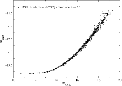
Figure 1: A sample of photographic (DSS-II red) fixed aperture (5″) magnitudes vs. CCD magnitudes. While the faint end gives us a linear relation, the core saturation of the bright stars lead to an asymptotic convergence to a constant value at the bright end.

Such a curve was ”invented” for the calibration of photographic densities by Moffat [1969]. He investigated in detail the calibration curves and the image growth of the stars on Hamburg Schmidt plates. We here use the equation of the same form

$$m_{\rm phot}=a_{0}\times\log\left({10^{a_{1}\times(m_{\rm CCD}-a_{2})}+1}\right)+a_{3}$$ (1)

where $m_{\rm phot}$ is the magnitude coming directly from the source extraction on the DSS or SuperCOSMOS plate, $m_{CCD}$ is the CCD magnitude corrected to the colour system of the plate and $a_{i};\,\,i\in[0,3]$ are free fit parameters. As we measure in case of stars an integrated value

$$\int_{0}^{R_{\rm aperture}}{f(T(r))\,r\,{\rm d}r}-\int_{0}^{R_{\rm aperture}}{f(S(r))\,r\,{\rm d}r}$$ (2)

were $T(r)$ is the really transmitted light in the measurement machine for the star and $S(r)$ that of the sky background. In the software we use the sky background is calculated as 2D polynomial in the region around the stellar aperture after exclusion of contamination by other sources. Details of this procedure can be found in Bertin & Arnaults (1996). This transmission is a function of seeing - and as shown by Moffat (1969) and Kimeswenger (1990) - strongly changes due to the wavelength dependent scattering within the plate. As shown already by Moffat and more in detail by Irwin & Hall (1983) simple fits of this growth function with e.g. Gaussians (as working fine for direct imaging CCDs) do not work well.

Assuming $a_{1}\rightarrow 1$ leads to the linearized ”Baker densities”. This works fine in case of some emulsion and wavelength domains (Hoffman et al. 1998). This fact was widely used to ”linearize” the calibration curves (e.g. the COSMAG values in the SuperCOSMOS catalogue) and to correct for the remaining deviation by semi-empirical functions (Hambly et al. 2001a). In fact this leads to ”global” parameters for the liberalization and free parameters fitting deviations. This is very suitable for global calibrations but not needed for the intended local calibration here.

But our main uncertainty in case of the public DSS data in fact is the unknown conversion function $f$ in the integration (Equ. 2) above. We measured the value of the unexposed plate (thereafter called chemical fog) and found strong variations from plate to plate. The machines were not calibrated in the same way all the time when scanning DSS2. Thus a general clear correlation of our fit parameters with the theoretical values by Moffat (1969) is not possible. This seems to be a major difference to the SuperCOSMOS scans, were all plates seemed to be scanned and calibrated in the same way. Therefore there is no way around a fitting of the parameters to obtain a proper solution.

While $a_{3}$ gives an estimate for the core saturation value, which strongly depends on the aperture size, $a_{0}\times a_{1}$ represents the inclination of the linear section, $a_{1}$ also influences the curvature around the knee and $a_{2}$ gives more or less the start of the linear section. An individual fit $m_{\rm phot}(m_{\rm CCD};a_{0},a_{1},a_{2},a_{3})$ for each CCD sequence and each aperture was derived. The correlation coefficient for all fits was always $R^{2}>0.995$. We derived the standard deviation of the fitted values $\sigma_{\rm f}$ in bins of $\Delta m=0\aas@@fstack{m}1$ for $m>12\aas@@fstack{m}0$. It is nearly negligible for bright sources and increases steadily towards the exposure limit. Near the limit the error will originate partly also from the CCD sequences (see Figure 2).

The reverse function of (1) then has to be used to derive the $m_{\rm CCD}$ of targets

$$m_{\rm CCD}={1\over a_{1}}\times\log\left({10^{(m_{\rm phot}-a_{3})\over a_{0}}-1}\right)+a_{2}$$ (3)

To derive an error estimate for the resulting magnitudes $\sigma_{\rm m}$ for the reverse function we used the derivative

$$\sigma_{\rm m}=\sigma_{\rm f}\left({{\rm d}m_{\rm phot}\over{\rm d}m_{\rm CCD}}\right)^{-1}={\sigma_{\rm f}\over a_{0}a_{1}}\left({1+10^{-a_{1}(m_{\rm CCD}-a_{2})}}\right)$$ (4)

This clearly leads to a very high effective error at the bright end of the calibration where the saturation effects the data. There the isophotal magnitudes are definitely better. But as we have shown in the introduction we are not interested in this part of the calibration as it can be reached better by other means. In Figure 2 the rms residuals for a fit are shown. For most of the brightness region of interest the error is about 0$\aas@@fstack{m}$1 or even below. Finally we tested whether the fits, respectively the residua are a function of the stellar colour. This test gives us information on the quality of the colour equations used.

Figure 2: The rms as function of magnitude for plate ER772 in the region around the variable star V838 Mon. The error mostly lies at or below 0$\aas@@fstack{m}$1. The slow increase towards the fainter end is partly denoted to the accuracy of the photoelectric sequence of Henden (2002). At the bright end the error increases rapidly due to the core saturation. The smaller ”jump” (at 14$\aas@@fstack{m}$5) is due to a ”cluster” of slightly blended stars around the target V838 Mon, having all about the same apparent magnitude. They also might have inaccurate CCD magnitudes, as the calibration sequence was taken during a bright outburst of the Target.

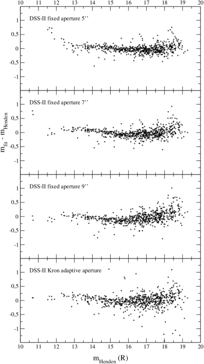
Figure 3: The deviation of fits with different apertures in the 15′$\times$15′field around V838 Mon.

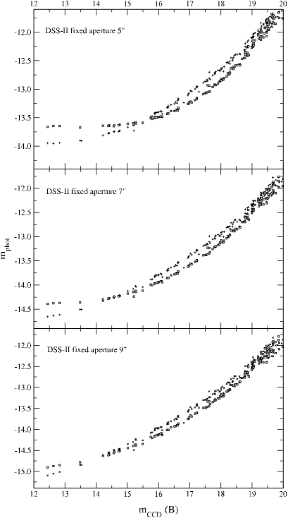
Figure 4: The field around the variable star AM Her on the plates XJ229 and XJ230. The overlapping region allows us to study the different behaviour of the plates individually.

The smaller the aperture we used, the smaller the error was (Figure 3) at higher magnitudes. On the other hand the saturation goes deeper. Often adaptive Kron apertures (Kron 1980) are used to avoid saturation. This method is also implemented in SExtractor. Comparing our result to the accuracy shows that the rms is larger at all wavelengths. Crowding seems to confuse too often the adaptive apertures. Kron adaptive apertures, using two or more threshold levels, are indeed a kind of profile fitting. As already pointed out by Irwin & Hall (1983), profile fitting leads to the highest errors. They find best results for isophotal photometry, while we find in our crowded fields in the galactic plane best results by using small apertures.

The solutions for the individual scans strongly differ from plate to plate. There is no general solution for the parameters. As shown in Figure 4 the plates are exposed and scanned so differently that neither the saturation ($a_{3}$) not the inclination at the higher magnitudes ($a_{0}\times a_{1}$) nor the curvature ($a_{1}$) or the position of the knee ($a_{2}$) is fixed somehow. Normally one does not have deep CCD sequences as we used here for the base study. Thus we tested the robustness of the fits with a small number of bright CCD calibrators. But in fact we were searching for an extrapolation if only a few bright CCD calibrators are available. We thus tried to derive some of the parameters by basic measurement on the plate itself. For this purpose we obtained the value of the unexposed plate $I_{F}$ at the plate edge (often called chemical fog), the value of the sky background $I_{S}$ and finally that of the overexposed plate $I_{O}$ in the center of a bright star nearby. All those measurements are used ”as is” in the published files. These units are the original natural analog/digital converter units folded by the (to the user unknown) function $f$ (see equation 2). Looking to equation (1) one can see that $a_{3}$ gives the magnitude of a star were the overexposed core is just as big as the (fixed size) aperture. Inserting the saturation and the sky level to equation (1) this leads together with the aperture $d$ (in units of pixels) to:

$$a_{3}=-2.5\log\left[{{\pi d^{2}\over 4}\,\left({I_{O}-I_{S}}\right)}\right]$$ (5)

In our tests we found a strict correlation of the chemical fog and the sky level with the parameter $a_{2}$. The dynamic range from the chemical fog to the sky level ($I_{S}-I_{F}$) gives us

$$m_{\rm phot}(a_{2})=-2.5\log\left[{{\pi d^{2}\over 4}\,\left({I_{S}-I_{F}}\right)}\right]$$ (6)

The CCD magnitude of a star with $m_{\rm phot}(a_{2})$ (or the mean of a set of stars within $m_{\rm phot}(a_{2})\pm 0\aas@@fstack{m}05$) is equal to $a_{2}$. This gives a limit for the deepness of the CCD sequence needed for the calibration.

Finally inserting the CCD magnitude of the curvature point $a_{2}$ into equation (1) we get with the two equations (5) and (6) above a solution for $a_{0}$

$$a_{0}=-{2.5\over\log(2)}\log\left[{{I_{S}-I_{F}}\over{I_{O}-I_{S}}}\right]$$ (7)

This parameter $a_{0}$ is independent from the aperture, as it describes the inclination of the curve at stars much smaller than the aperture. As we now were able to fix 3 (out of 4) parameters, the fit of the remaining parameter $a_{1}$ was robust against reducing the number and the limiting magnitude of the calibrators.

Figure 5: The evolution of the fits of parameter $a_{1}$ as function of the limiting magnitude. It converges to the optimum at magnitudes around $a_{2}$ which was derived independently before as described above.

Figure 5 shows that the limiting magnitude for the CCD sequence has to be deep enough to reach the value of $a_{2}$ derived above. Deeper sequences do not improve the quality of the parameter anymore. Thus a real extrapolation from bright CCD sequences to faint stars is possible (see Figure 6).

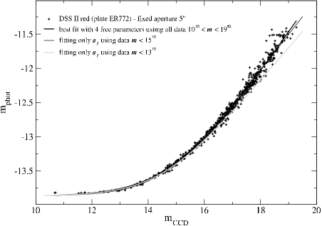
Figure 6: The real 4 parameter fit is nearly identical with the fit fixing 3 parameters and using the sequence up to $m_{\rm CCD}=15\aas@@fstack{m}0$. Even the fit with very bright calibrators only, although systematically wrong at the faint end, does not deviate more than about 0$\aas@@fstack{m}$5 - the rms found often for globally calibrated astrometric surveys like e.g. USNO B.

4 The H-compression

The DSS data is compressed by the use of a ”lossy” algorithm. The H-compression (White et al. 1992) uses typical factors of 5 in crowded fields and up to 10 at high galactic latitudes (Lasker et al. 1996). We investigated the influence of the H-compression in one field around the suspected symbiotic variable star V471 Per. For comparison the plate from the SuperCOSMOS data archive, scanned at much higher resolution of 0$\aas@@fstack{\prime\prime}$67, was median filtered 3$\times$3 pixels ($\equiv$ 1$\aas@@fstack{\prime\prime}$98$\times$1$\aas@@fstack{\prime\prime}$98) and then rebinned to the DSS pixel size of 1$\aas@@fstack{\prime\prime}$01. A CCD calibration sequence is given by Henden & Munari [2001]. The result in Figure 7 shows that there is no degeneration of the photometry even down to the plate limit. The rms of the regression is below 0$\aas@@fstack{m}$09 at $m<20\aas@@fstack{m}0$ and increases to 0$\aas@@fstack{m}$14 at $20\leq m<21\aas@@fstack{m}5$.

Figure 7: The photometry achieved on uncompressed (SuperCOSMOS plate rebinned to DSS resolution) vs. DSS-II H-compressed images around the suspected variable star V471 Per using the method described in section 3. There is obviously neither a systematic effect nor any degrading of the photometric quality.

5 Comparing to survey calibrations

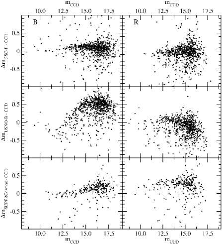
Figure 8: The deviation of the magnitudes given in the USNO-B catalog (Monet et al. 2003), the GSC 2.2 (STScI, 2001), and the SSS catalog (Hambly et al. 2001a) from those of Henden (2002) in the 15′$\times$15′field around AM Her.

Recently a set of globally calibrated surveys was released. While the GSC-II (http://www-gsss.stsci.edu/gsc/gsc2/GSC2home.htm) is based on the same scans (but before H-compression) we used for our investigation, the USNO-B catalog (Monet et al. 2003) and the SSS catalog (Hambly et al. 2001a) used data from different scanning machines. The USNO-B only uses an 8-bit linear converter for the transmitted light. This undersamples the greyscale variations in the centre of the stellar images. As already pointed out by Monet et al. (2003), the photometry never was a main goal of this survey. The SSS uses scans with a linear 15-bit greyscale from a CCD. The data is pre-calibrated using an average slope for the so called linear part of the emulsion of $\gamma=2$. Then a complex post-processing including CCD calibrators and colors is started (Hambly et al. 2001a). This is essential for wide area statistical studies, but not needed in our local calibration of individual sources. The comparison of the Henden (2002) CCD sequences with these catalogues for two of our fields is shown in Figs. 8 & 9.

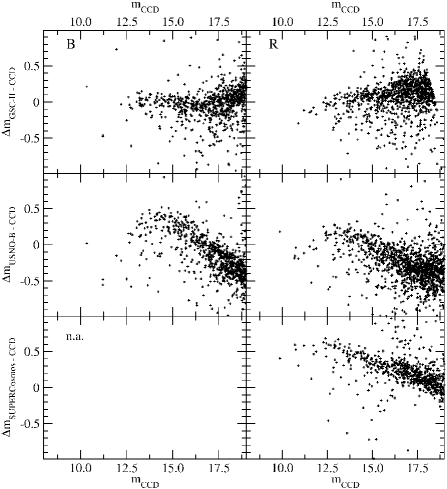
Figure 9: The deviation of the magnitudes given in the USNO-B catalog (Monet et al. 2003), the GSC 2.2 (STScI, 2001), and the SSS catalog (Hambly et al. 2001a) from those of Henden (2002) in the 15′$\times$15′field around V838 Mon.

The GSC2.2 do show a much higher noise but (nearly) no systematic effects. The calibration is not well documented in the literature neither at the survey homepage. Manual inspection of the sources in our fields leads us to the conclusion that at least a part of this error is originating from improper deblending of faint sources. The typically higher crowding on the red survey plates thus causes a higher error there.

The USNO-B photometry is based on extrapolation of bright TYCHO stars and a few faint calibrators on some plates. Finally the remaining plates were adjusted using the overlaps. We find generally very high ($\geq 0\aas@@fstack{m}5$) systematic deviations for all our fields.

The SSS uses a grid of faint CCD calibrators fields to define an average gradient of the isophotal magnitudes vs. CCD magnitudes. These were used to extrapolate towards the plate limit the individual field-by-field calibration curves derived from bright standards. Post-processing by a complex color classification and the plate overlaps were used to do fine-tuning (Hambly et al 2001a). The comparison with our results in the small fields leads to a much lower scatter than the surveys mentioned before. But systematic effects are sometimes evident. This is already pointed out by Hambly et al.: ”The isophotal scale is non linear at the level of $>$ 0.5 mag; furthermore, such non linearities are not repeatable from field to field.”

In a recent investigation of a field around the eruptive variable V4332 Sgr (Kimeswenger, 2005) another effect was crucial. The SSS, using the selection flags for high quality (= default), misses targets near bright stars (Figure 10). Also deblending, which works fine in SExtractor V2 (Bertin & Arnouts 1996), is not implemented to GSC-II and SSS properly.

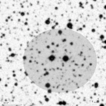
XX

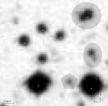
Figure 10: Left: The SSS avoids in the ’full-quality’ catalogue the region around bright stars (shaded area). This causes targets like here V4332 Sgr being missed; Right: SSS and GSC-II do not deblend targets, which are properly done by the neuronal network software SExtractor (elliptical areas). Also faint stars having a good S/N ratio nearby bright stars are ignored (polygonal area).

The calibration of the stars around V4332 Sgr by using ESO NTT CDD images (limiting mag $\approx$ 24$\aas@@fstack{m}$0) obtained by SK gives, after manual cleaning blends and all stars in the vicinity of 10” around bright stars a very good result for GSC-II. Again the SSS has strong systematic deviations (Figure 11).

Figure 11: The GSC-II and the SSS red magnitudes in a field around the eruptive variable V4332 Sgr (Kimeswenger, 2005).

6 Alternative calibration - CCD vs. GSC-II

As shown in the previous section the GSC-II, although having a higher rms error, shows nearly no systematic effects. Thus we tested a calibration by use of the GSC-II instead of the CCD sequence. This might be of interest in regions were no CCD calibrations are available or for a first quick result - e.g. especially after erruptive nova and nova like events. In Figure 12 the results of a calibration using a CCD sequence and alternatively using only the GSC-II to derive the $a_{i}$ parameters are shown. The results are promising. The systematic effects are significantly below the noise. The accuracy of such a local ”post-processing” of the GSC-II improves the photometry significantly.

Figure 12: Calibration of the field around V838 Mon using the CCD sequence (upper panel) and using GSC-II (lower panel).

7 Conclusions

The method we present here is well suited to calibrate locally even H-compressed digital sky survey data by just using a few bright calibrators. These calibrators easily can be achieved by using small amateur telescopes. The accuracy is about 0$\aas@@fstack{m}$1 for a wide range. Thus also colour-colour diagrams are possible. This allows to do photometry of progenitors for eruptive events like novae as well as HR diagrams when searching for new candidates for stellar clusters. The importance for variable and eruptive star studies was pointed out recently by Munari et al. [2002], Kimeswenger et al. [2002a] and Kimeswenger & Lechner [2003]. Goranskij et al. [2004] shows the strong implications on physical models of such kind of DSS usage. As pointed out by Kimeswenger [2005] several different epochs by using e.g. overlaps, not included all to the surveys, give us important information for such variable objects. Here we do not focus on light curves of variables on a set of (similar) plates with respect to a reference plate. In such a case photometric differential work is usually the best choice. Comparing single epoch data or data on different bands (e.g. POSS-I and POSS-II blue are different) with new CCD data the progenitors of eruptive variables indeed need absolute calibration. But also the investigations of small dark clouds by Stüwe [1990], who used statistical calibrations with a BS model (Bahcall & Soneira 1984) and complementary galactic structure work like that of Curry & McKee [2000] and of Castellani et al. [2001] might be improved by this kind of calibrations presented here.
The local calibration presented here is clearly not overcoming global surveys (e.g. Hambly et al. 2001a or Monet et al. 2003) for large statistical samples, but due to the higher accuracy (restricted to small fields) a perfect access for studies of individual targets is provided. Also the follow up whether stellar concentrations are newly detected clusters or similar work may be done without using mid size telescopes (e.g. Boeche et al. 2003).

References

- [2001] Andersen M., Kimeswenger S., 2001, A&A, 377, L5
- [2001] Bacher A., Lederle C., Grömer G., Kapferer W., Kausch W., Kimeswenger S., 2001, IBVS, 5182
- [1984] Bahcall J.N., Soneira R.M., 1984, ApJS, 55, 67
- [1996] Bertin E., Arnouts S., 1996, A&AS, 117, 393
- [1982] Blair M., Gilmore G., 1982, PASP, 94, 742
- [2003] Boeche C., Barbon R., Henden A., Munari U., Agnolin P., 2003, A&A, 406, 893
- [2001] Castellani V., Degl’Innocenti S., Petroni S., Piotto G., 2001, A&A, 324, 167
- [2000] Curry C.L., McKee C.F., 2000, ApJ, 528, 734
- [2004] Goranskij V.P., Shugarov S.Yu., Barsukova E.A., Kroll P., 2004, IBVS, 5511
- [2001a] Hambly N.C., Irwin M.J., MacGillivray H.T., 2001a, MNRAS, 326, 1295
- [2001b] Hambly N.C., MacGillivray H.T., Read M.A., et al., 2001b, MNRAS, 326, 1279
-
[2002]
Henden A.A., 2002,
ftp://ftp.nofs.navy.mil/pub/outgoing/aah/sequence/ - [2003] Henden A.A., 2003, private communication
- [2001] Henden A., Munari U., 2001 A&A, 372, 145
- [1998] Hoffmann B., Tappert C., Schlosser W., Schmidt-Kaler Th., Kimeswenger S., Seidensticker K., Schmidtobreick L., Hovest W., 1998, A&AS, 128, 417
- [1992] Hörtnagl A.M., Kimeswenger S., Weinberger R., 1992, A&A, 262, 369
- [1991] Humphreys R.M., Landau R., Ghigo F.D., Zumach W., Labonte A.E., 1991, AJ, 102, 395
- [1983] Irwin M.J., Hall P., 1983, in Workshop on Astronomical Measuring Machines, Edinburgh, Proceedings (A83-50001 24-89). Edinburgh, Royal Observatory, 1983, p. 111
- [1990] Kimeswenger S., 1990, PhD thesis, University Bochum, Germany
- [2001] Kimeswenger S., 2001, AGM, 18, 251
- [2005] Kimeswenger S., 2005, AN, submitted
- [2003] Kimeswenger S., Lechner M.F.M, 2003, A&A, 411, L461
- [2002a] Kimeswenger S., Lederle C., Schmeja S., Armsdorfer B., 2002a, MNRAS, 336, L43
- [2003] Kimeswenger S., Lederle C., Armsdorfer B., Pritchard J., 2003, Rev. Mex. Astron. Astroph., 39, 35
- [2002b] Kimeswenger S., Schmeja S., Kitzbichler M.G., Lechner M.F.M., Mühlbacher M.S., Mühlbauer A.D., 2002b, IBVS, 5233
- [2001] Kimeswenger S., Weinberger R., 2001, A&A, 370, 991
- [1981] King D.J., Birch C.J., Johnson C., Taylor K.N.R., 1981, PASP, 93, 385
- [1980] Kron R.G., 1980, ApJS, 43, 305
- [1996] Lasker B.M., Doggett J., McLean B., Sturch C., Djorgovski S., de Carvalho R.R., Reid I.N., 1996, ASP Conf. Ser., 101, 88
- [1990] Lasker B.M., Sturch C.R., McLean B.J., Russell J.L., Jenkner H., Shara M.M., 1990, AJ, 99, 2019
- [1994] Lasker B.M., McLean B.J., 1994, STSci Newsletter, 11, No. 2, 39
- [1988] Lasker B.M., Sturch C.R., Lopez C., et al., 1988, ApJS, 68, 1
- [2003] Lederle C., Kimeswenger S., 2003, A&A, 397, 951
- [1969] Moffat A.F.J., 1969, A&A, 3, 455
- [2002] Munari U., Henden A., Kiyota S., et al., 2002, A&A, 389, L51
- [2003] Monet D.G., Levine S.E., Canzian B., et al., 2003, AJ, 125, 984
- [1997] Morrison, J.E., Lasker B., McLean B., Bucciarelli B., Spagna A., Zacchei A., 1997, Proceedings of the ESA Symposium ‘Hipparcos - Venice ’97’, 13-16 May, Venice, Italy, ESA SP-402 (July 1997), 402, 129
- [1991] Reid I.N., Brewer C., Brucato R.J., et al., 1991, PASP, 103, 661
- [1982] Reid N., Gilmore G., 1982, MNRAS, 201, 73
- [1990] Russell J.L., Lasker B.M., McLean B.J., Sturch C.R., Jenkner H., 1990, AJ, 99, 2059
- [1996] Spagna A., Lattanzi M.G., Lasker B.M., McLean B.J., Massone G., Lanteri L., 1996, A&A, 311, 758
- [1990] Stüwe J.A., 1990, A&A, 237, 178
- [1992] White, R.L., Postman, M., Lattanzi M.G., 1992, in Digitised Optical Sky Surveys, eds. H.T. MacGillivray & E.B. Thompson, Dordrecht, Kluwer, p. 167