Phosphorus in the Diffuse Interstellar Medium

We present FUSE and HST/STIS measurements of the P ii column density toward Galactic stars. We analyzed P ii through the profile fitting of the unsaturated $\lambda$1125 and $\lambda$1533 lines and derived column densities integrated along the sightlines as well as in individual resolved components. We find that phosphorus is not depleted along those sightlines sampling the diffuse neutral gas. We also investigate the correlation existing between P ii and O i column densities and find that there is no differential depletion between these two specie. Furthermore, the ratio $N$(P ii)/$N$(O i) is consistent with the solar P/O value, implying that P ii and O i coexist in the same gaseous phase and are likely to evolve in parallel since the time they are produced in stars. We argue that phosphorus, as traced by P ii, is an excellent neutral oxygen tracer in various physical environments, except when ionization corrections are a significant issue. Hence, P ii lines (observable with FUSE, HST/STIS, or with VLT/UVES for the QSO sightlines) reveal particularly useful as a proxy for O i lines when these are saturated or blended.

1 Introduction

Phosphorus (${}^{31}_{31}$P) is an odd-Z element which is thought to be mainly produced in the same massive stars that form $\alpha$-elements (O, Ne, Mg, Si, S, Ar, …). Although the nucleosynthesis of odd-Z elements is still not well understood, phosphorus seems to be produced during the carbon and neon burning in a hydrostatic shell (Arnett 1996). Woosley & Weaver (1995) found that no significant amount is expected to be synthesized during the explosion phases and that the P yields should be metallicity dependent because of the odd–even effect.

In the Galactic and extra–galactic diffuse interstellar medium (ISM), the phosphorus gaseous phase abundance is largely unknown. Apart from the early investigations with the Copernicus satellite within the solar neighborhood (Jenkins et al. 1986; Dufton et al. 1986), quite a few measurements are available in the distant ISM and almost none in the extragalactic ISM. Nevertheless, the ISM phosphorus abundance provides an important constraint for the dust/gas chemistry.

Dust grains are subject to dramatic chemical, morphological, and structural changes during their life time, from the condensation of dusty cores within the outflows of evolved stars to the final destruction in shocks or the formation of new generations of stars and planetary systems. They undergo several growth (mantle accretion and molecules adsorption) and erosion (photoprocessing, sputtering) periods as they move within dense or diffuse media (Snow & Meyers 1979; Seab 1987; Turner et al. 1991; O’Donnell & Mathis 1997). In that respect, refractory elements are expected to be the most depleted in the gas phase. On the contrary, C, N, and O are less depleted onto dust grains because of their lower condensation temperatures (Field 1974; Lodders 2003). Hence, one third of the oxygen is bound to rocky elements at most (Cardelli et al. 1997). With respect to its relatively high condensation temperature, phosphorus can be expected a priori to be more heavily depleted.

Jenkins et al. (1986), in their ISM survey conducted with Copernicus toward about 80 stars, found through the analysis of the far-UV absorption lines of the dominant ion stage P ii that phosphorus is not depleted along sightlines containing predominantly warm low density neutral gas ($\lesssim$0.1 dex after updating the solar abundances from Asplund et al. 2004) and is depleted by $\lesssim$0.5 dex in cooler and denser clouds. Using the same dataset but with a different oscillator strength for the P ii $\lambda$1302 transition, Dufton et al. (1986) derived phosphorus abundances systematically larger by $\approx 0.2$ dex so that the previous findings still hold. Finally, it must be added that in the cold diffuse interstellar cloud toward $\zeta$ Oph, the depletion of phosphorus is $0.5\pm 0.2$ dex as compared with $0.4\pm 0.1$ dex for oxygen, while in the warm diffuse cloud along the same sightline, P is depleted by $0.2\pm 0.1$ dex as compared with $0.0\pm 0.3$ dex for O (Savage & Sembach 1996).

The first detection of the PN molecule by Turner & Bally (1987) through the 140 GHz ($J=3-2$) and 234 GHz ($J=5-4$) emission lines paved the way to extensive studies of the abundance of phosphorus in molecular clouds. It was soon recognized that the transfer of phosphorus from the gas to the solid and back to the gas phase was largely involving carbon atoms via the HCP linear molecule (Turner et al. 1990). As a consequence, phosphorus is believed to mainly reside in adsorbed HCP molecules which are then released in the gas by photodesorption in warm media and readily photodissociated. This scenario would account for the lack of depletion in the warm phase.

Since the advent of the Far Ultraviolet Spectroscopic Explorer (FUSE) satellite (Moos et al. 2000) and the STIS instrument onboard HST, it is now possible to probe denser clouds and investigate longer sightlines. We thus revisit and extend previous works on interstellar phosphorus abundance by presenting new P ii measurements toward Galactic sightlines obtained from FUSE and HST/STIS data. Furthermore, in order to point out the relative behavior of phosphorus as compared with $\alpha$-elements and possibly reveal a global trend toward the differential depletion under many different physical conditions, we compare the phosphorus gaseous phase abundance with that of oxygen. Oxygen abundance in the diffuse ISM has been extensively studied over the last years (see e.g., Jensen et al. 2005, Cartledge et al. 2001, Cartledge et al. 2004, and André et al. 2003 $-$ hereafter A2003) and is used here as a reference element. The observations and data analysis are described in Sections 2 and 3. We present the results in Sect. 4. Final conclusions are given in Sect. 5.

2 Observations

We have selected 10 sightlines toward Galactic stars with distances up to $\approx 5$ kpc in order to scan the distant ISM. Properties of the targets and the sightlines are summarized in Table 1. Tables 2 and 3 provide the log of the FUSE and HST/STIS observations, respectively. Given the Galactic latitudes and distances of the stars, all the sightlines intersect clouds in the Galactic disk, except the sightline toward HD121968 which possibly can intersect clouds in the halo.

All the FUSE spectra were obtained through the large 30″$\times$30″ (LWRS) aperture which results in a resolving power $R\equiv\lambda/\Delta\lambda\approx 20,000$ (or $\Delta v\approx$ 15 km s^-1, FWHM). This spectral resolution depends on the co–addition procedure used to reconstruct the total exposure and varies with the wavelength and the detector. Hence, we did not attempt to co–add different detectors, in order to minimize both the distortion of the resulting Point Spread Function (PSF) and the propagation of the Fixed Pattern Noise (FPN) proper to each detector. The detailed reduction, calibration and co–addition procedures can be found in A2003 who reduced most of the present data in order to study the neutral oxygen and hydrogen content along the sightlines.

The STIS observations were taken with the far-ultraviolet MAMA detector equipped with the E140H grating. However, three different apertures were used. The $0\aas@@fstack{\prime\prime}1\times 0\aas@@fstack{\prime\prime}03$ aperture provides a resolving power $R\approx 200,000$ (or $\Delta v\approx 1.5$ km s^-1, FWHM). The two others, $0\aas@@fstack{\prime\prime}2\times 0\aas@@fstack{\prime\prime}09$ and $0\aas@@fstack{\prime\prime}2\times 0\aas@@fstack{\prime\prime}2$, provide a spectral resolution of $R\approx 110,000$ (velocity resolution of $\Delta v\approx 2.7$ km s^-1, FWHM). Again, details about the data reduction can be found in A2003.

Among the 10 targets we present, 8 were analyzed by A2003 with a particular concern on the O i column density. The other targets of their sample were not observed with STIS at the wavelength of the P ii $\lambda$1533 line (see next section). Furthermore, we analyzed STIS spectra of two additional targets, HD24534 and HD121868.

Finally, we also compiled published P ii and O i measurements in the Milky Way and along a few extragalactic sightlines. These are listed in Table 6 and discussed in Sect. 4.3.

3 Data analysis

Because of the ionization potential of O i (13.62 eV as compared with 13.60 eV for H i) and the efficient charge exchange between O ii and H i, O i is expected to be the dominant ionization state of oxygen in the diffuse neutral gas, and thus a good tracer of the neutral gas. Observations of A2003 confirm this finding. On the other hand, the ionization potentials of P i and P ii (resp. 10.49 eV and 19.72 eV) suggest a priori that P ii should be the dominant state of phosphorus in this gaseous phase. However a fraction of P ii atoms could actually reside in a potential ionized gaseous phase where oxygen is into O ii and hydrogen into H ii. The fraction is unknown and depends on the ionizing radiations illuminating the diffuse clouds. The present study will help to identify this possible correction.

Absorption lines were analyzed assuming Voigt profiles, by using the profile fitting program Owens. This fortran code, developed by M. Lemoine and the FUSE French team, is particularly suitable for simultaneous fits of far-UV spectra (Lemoine et al. 2002). A great advantage of this routine is the ability to fit different spectral domains and various species in a single run. It was then possible to analyze simultaneously the P ii and O i absorption lines, together with Cl i, C i, and S i lines. The use of these species in a simultaneous fit allowed us to check and constrain the radial velocity structure of the sightlines when uncertain. The P ii and O i lines we analyzed being unsaturated, the column density determination does not depend on the $b$-parameter. The errors on the column densities are calculated using the $\Delta\chi^{2}$ method described in Hébrard et al. (2002) and include the uncertainties on all the free parameters such as the continuum shape and position. All the errors we report are within 1 $\sigma$.

Numerous O i lines are observed in the HST/STIS $+$ FUSE spectral ranges, with oscillator strengths ($f$) spanning several orders of magnitude. However, the main constraint on the O i column density consists in using the weak 1355.5977 Å intersystem transition ($f=0.116\times 10^{-5}$). The total O i column densities toward most of the present sightlines were derived by A2003 using this line. However, we have updated these values by deriving column densities of each cloud along the sightlines and by performing a simultaneous analysis of O i and P ii lines.

A total of seven P ii lines are available in the far-UV spectral domain. Thanks to the combination of datasets, the phosphorus atoms content is readily explored through transitions spanning more than 2 orders of magnitude in oscillator strengths, always allowing the choice of adequat lines for a particular study. Wavelengths and $f$-values are from the revised compilation of atomic data by Morton (1991; 2003). One must be aware that oscillator strengths of P ii lines could be relatively uncertain. Indeed, phosphorus atomic data have been poorly investigated and no laboratory experiments exist.

In the present study, the three P ii lines at 961.0412 Å ($f=0.349\times 10^{0}$), 963.8005 Å ($f=0.146\times 10^{1}$) and 972.7791 Å ($f=0.210\times 10^{-1}$), observable with FUSE, are located in a region overcrowded with strong absorption lines $-$ mainly H i lines from the Lyman serie and H₂ lines. We thus rejected these transitions because blended. In addition, the two first lines are heavily saturated, thus preventing reliable P ii column determinations.

Similarly, we avoided the P ii lines at 1152.8180 Å ($f=0.245\times 10^{0}$, observable with FUSE), and at 1301.8743 Å ($f=0.127\times 10^{-1}$, observable with STIS) since they both present most of the time saturation effects. It must be added that the later is most often blended with the extremely strong O i line at 1302.1685 Å, even at the highest STIS resolution.

The P ii line at 1124.9452 Å ($f=0.248\times 10^{-2}$, observable with FUSE) is the weakest transition available and is always found to lie on the linear part of the curve of growth. When detected, it can provide an accurate measurement of the total phosphorus column density along a given sightline but with little information on the velocity structure. One should note that analyzing this line requires high–quality data and a good knowledge of FPN for the FUSE detectors. Indeed, duplicate detectors make more easy to discriminate FPN and absorption features in most cases. Unfortunately, in some cases this line appears slightly blended with the broad Fe iii* $\lambda$1124 stellar line.

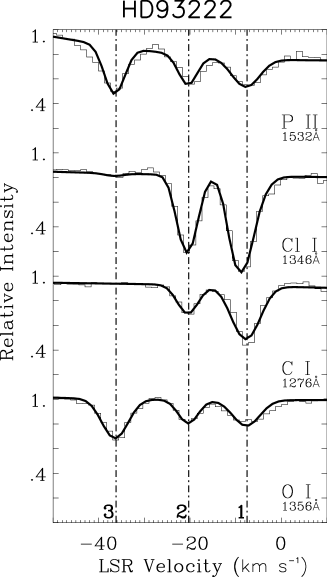
Figure 1: P ii $\lambda$1533 absorption line profile toward HD93222. Three components are easily identified. When detected, Cl i, C i, and S i lines are used to constrain the velocity distribution (turbulent velocity and radial velocity). P ii and O i lines have very similar optical depths since the $N\cdot f$ product is approximately the same (see text).

Slightly stronger is the P ii line at 1532.5330 Å ($f=0.303\times 10^{-2}$, observable with STIS). Thanks to the STIS higher resolution, this line allows the investigation of the detailed velocity distribution of sightlines and the derivation of phosphorus column densities in individual clouds. We thus used this line to derive the P ii column densities (column density of each individual clouds and integrated column density over the sightline) and compare with the O i values. The other great and main advantage of this line is that its optical depth is systematically found to be similar to the optical depth of the O i $\lambda$1356 line (see Fig. 1). This is due to the combination of the O i column density, about 2000 times larger than the P ii one, and the oscillator strength, 2000 times lower than for the P ii $\lambda$1533 line. Hence, the simultaneous analysis of these two lines minimizes possible systematic errors due to possible saturation and/or unresolved components. This combination further allows to investigate individual cloud column densities since these two lines are observed in the same high-resolution dataset.

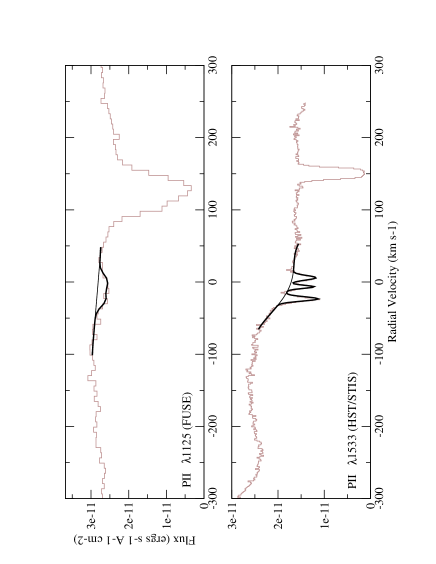
Figure 2: Plot of the P ii $\lambda$1125 line toward HD93222 as observed with FUSE (top) and of the $\lambda$1533 line as observed with STIS (bottom). The two lines have approximately the same oscillator strength. Given the relatively low spectral resolution, the FUSE observation allow to calculate the integrated column density along the sightline while the STIS observation gives the possibility to investigate column densities of each component.

Another possibility consists in comparing the integrated column density as derived from the unresolved profile of the P ii $\lambda$1125 line with FUSE, with the sum of the P ii column densities of individual clouds along the sightlines as derived with the STIS resolved profile of the P ii $\lambda$1533 line (Fig. 2). We get consistent findings within the error bars (see Table 4). This comparison provides a twofold confirmation: 1) the relative compatibility of the corresponding oscillator strengths, and 2) the absence of gross systematic errors when assuming only one global velocity component to estimate integrated column densities.

4 Results

4.1 Abundance of phosphorus

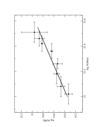
Figure 3: Plot of the P ii column density integrated over each sightline versus the total hydrogen column density defined as $\log[N(\textrm{H\,{\sc i}})+2\times N(\textrm{H}_{2})]$. The thick line shows the solar phosphorus abundance (Asplund et al. 2004) and the thin dashed line shows the regression fit.

We plot in Fig. 3 the integrated P ii column density (as derived with the P ii $\lambda 1532$ line) versus the total hydrogen content defined as $N$(H${}_{\textrm{tot}}$)=$N$(H i)$+2\times N$(H₂). We use the values $N$(H i) and $N$(H₂) derived by A2003 through FUSE observations, available for 8 of our 10 sightlines. Column densities are integrated along sightlines and sample the diffuse ISM. As compared with the solar abundance $\log$ (P/H)_⊙=$-6.65\pm 0.04$ (Asplund et al. 2004), the regression of P ii vs. H${}_{\textrm{tot}}$ gives a consistent value $-6.64\pm 0.05$. We can conclude that:

• Phosphorus is not depleted in the diffuse neutral ISM up to at least $\log N$(H${}_{\textrm{tot}}$)$\approx 21.5$ and $E$(B-V)$\approx 0.5$,

• P i exist only in negligible amounts in this gaseous phase since we would observe an even higher P/H ratio. P ii is indeed the dominant state of phosphorus along these 8 sightlines.

Of course, these findings must be tempered by the fact that we used the integrated column densities along the sightlines. As a matter of fact, P ii column densities can be derived for individual clouds (see next section), but unfortunately, it is not possible to do the same for hydrogen, given the relatively large width of the H i absorption lines observed with FUSE and HST/STIS.

4.2 Phosphorus versus oxygen

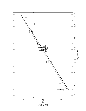
Figure 4: P ii total column density over each sightline is plotted versus the total O i column density. The thick line shows the solar ratio (Asplund et al. 2004) and the thin dashed line shows the regression fit.

The integrated P ii and O i column densities toward the 10 Galactic sightlines of our sample were derived using the P ii $\lambda 1533$ and O i $\lambda 1356$ lines, observable with STIS. Values are listed in Table 4 and plotted in Fig. 4. We find consistent integrated O i column densities within 1 $\sigma$ error bars with those found by A2003 except toward a few sightlines for which error bars of A2003 could have been somewhat underestimated. There are also some overlap with other past measurements (see Howk et al. 2000, Jensen et al. 2005, and Knauth et al. 2003). These past values are marginally consistent with our values within 1 $\sigma$ error bars, except the O i column density toward HD218915 derived by Howk et al. (2000). However, this Howk et al. determination is also inconsistent with the other studies of A2003 and Knauth et al. 2003.

There is a clear correlation between P ii and O i column densities. The derived error-weighted mean P ii/O i ratio is $-3.26^{+0.12}_{-0.10}$ (1 $\sigma$ error bars), which is consistent with the solar P/O proportion $-3.30\pm 0.07$ (Asplund et al. 2004). The only exception is the sightline toward the star HD121968 located in the halo. We observe a single absorption component which could arise in a cloud located in the low-density partly-ionized Galactic halo. Therefore, in such extreme conditions, P ii could also exist where oxygen is ionized so that the actual P/O ratio would be $\eta\times N$(P ii)/$N$(O i), where $\eta<1$ is an unknown factor which depends on the ionization conditions within the cloud. This ionization effect is negligible for all the other sightlines.

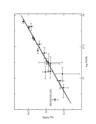
Figure 5: P ii column density of each individual component along the sightlines plotted against the corresponding O i column density. The thick line shows the solar ratio (Asplund et al. 2004) and the thin dashed line shows the regression fit.

Does the same correlation hold if we plot the column densities of individual clouds along the sightlines ? We selected individual components in each sightline on the basis of a clear separation from nearby other absorptions $-$ i.e. the wavelength shift due to the different radial velocities of clouds must be larger than the intrinsic line widths (convolution of the turbulent velocity and the instrumental line spread function). We identified 17 interstellar absorbing regions along our sightlines (Table 5). We still find a correlation over more than $\approx$1 dex in column density (Fig. 5), with a mean P ii/O i ratio of $-3.25^{+0.12}_{-0.10}$, again consistent with the solar P/O ratio. The only noticeable exception to this good correlation (apart from the single component along the HD121968 sightline, see above) is the component #2 along the HD104705 sightline. This sightline crosses an interarm region in the Milky Way disk where the medium is particularly ionized (Sembach 1994). This strongly suggests that the absorption component #2 lies in such a region where P ii/O i is larger than the actual P/O ratio.

Given these correlations, the following conclusions can be put forward:

• There is no clear evidence of a differential depletion of P ii and O i in the diffuse neutral gas sampled here. This is true over all the range of molecular fraction $f$(H₂) = 0.05-0.28 and reddening $E$(B-V) = 0.17-0.53.

• P ii and O i coexist in the same gaseous regions; no ionization correction seems to be required, except in two ionized interstellar clouds. Phosphorus and oxygen are thus likely to evolve in parallel in the ISM since the time they are produced in stars and to be well mixed.

• Finally, the oscillator strength of the P ii $\lambda$1533 line seems to be well defined and compatible with the $f$-value of the $\lambda$1125 line (see Sect. 3).

4.3 Measurements in various physical environments

We gathered from the literature several Galactic and extragalactic sightlines toward which both P ii and O i column densities have been measured (see Table 6). We have excluded two sightlines toward subdwarf O stars (Wood et al. 2004) since the P ii column densities were determined through only one saturated line.

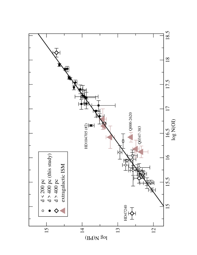
Figure 6: Compiled measurements of P ii and O i column densities found in the literature (see Table 6) overplotted on our results. Empty circles represent sightlines toward stars with distances less than 200 pc. Filled circles represent the values of this study (results plotted in Fig. 5 toward stars between $\approx 400$ and $\approx 5000$ pc), and diamonds represent values found in the literature toward stars with comparable distances. Finally, triangles show measures in the extragalactic ISM. The thick line represent the solar P/O proportion (Asplund et al. 2004).

The sightlines are quite various in terms of distances to the targets. We list indeed twenty stars, from the Local Bubble (within 100 pc) to the distant Galactic plane (with star distances up to 5 kpc), one star in the Small Magellanic Cloud, and four high-redshift damped Lyman $\alpha$ systems (DLAs). The sightlines also span various metallicities (from solar to $\sim 1/100$ solar) and various color excesses. All these values are overplotted on our results in Fig. 6. The correlation between P ii and O i column densities found in Sect. 4.2 still holds over more than three decades in column densities.

We notice however that in three DLAS, the P ii/O i column density ratio is significantly lower than the solar P/O value. This could be the sign of a metallicity dependence of P ii/O i although the measures in other low metallicity environments give solar values (Table 6). On contrary, Welsh et al. (2001) found a relatively high P ii/O i ratio in the high velocity gas toward HD47240, lying just behind the Monoceros Loop Supernova Remnant (SNR). This high ratio could be explained by the ionization effects of the SNR gas found by the authors.

The derived error-weighted mean P ii/O i ratio of all these data points is $-3.28^{+0.15}_{-0.13}$, again consistent with the solar P/O value. Results of previous section are thus confirmed and reinforced since P ii/O i appears to be relatively homogeneous, at least within the Milky Way over nearly 5 kpc.

As a conclusion, it is thus reasonable to propose that phosphorus, as traced by P ii, can be used to trace O i column density in the diffuse ISM since there is no clear sign of differential depletion.

5 Conclusions

We investigated 10 Galactic sightlines and found that:

• P ii is a good tracer of the neutral gas in most interstellar clouds and can be used as a proxy to derive the phosphorus abundance in this gaseous phase. Ionization seems to be an issue only in extreme conditions.

• There is no depletion of phosphorus in the diffuse neutral medium toward these stars.

• P ii and O i column densities relate to each other in solar P/O proportions. There is no differential depletion of P ii and O i.

• The oscillator strengths of the P ii $\lambda$1125 and P ii $\lambda$1533 lines do not suffer from significant misestimates.

Our results suggest in particular that phosphorus could be an ideal tracer of oxygen in extragalactic regions. Oxygen is indeed of prime importance to understand the chemical evolution of galaxies. It is one of the most abundant element in the Universe and its nucleosynthesis is well known. Its abundance is therefore widely used to estimate the metallicity of different Galactic and extragalactic ISM gas phases. Oxygen has been in particular extensively investigated to derive H ii region metallicities. However, in the neutral phase, oxygen abundance in extragalactic regions is often poorly constrained. Indeed, the O i lines detected in blue compact dwarfs (BCDs) and in giant H ii regions of spiral galaxies are often saturated resulting in large error bars on the metallicity determinations. Among the BCDs for which the neutral gas have been probed so far with FUSE, several suffer from large systematic errors on their O i column densities, complicating a further interpretation. The errors on $\log$ (O i/H i) are generally larger than $\pm 0.5$ dex (Lecavelier et al. 2003, Thuan et al. 2002, Thuan et al. 2005, Lebouteiller et al. 2004, Cannon et al. 2003). To circumvent this issue, the use of phosphorus could be a interesting new way to estimate the oxygen abundance, provided ionization corrections are not needed. However, note that if the spread of the P ii/O i ratio is only due to ionization and not to depletion or other effects, it can reveal a useful constraint to the ionization corrections in diffuse clouds. Finally, he present study is too limited to answer the question of the metallicity dependence of the P ii/O i ratio. Therefore, we cannot conclude without ambiguities on the use of phosphorus in low-metallicity environments such as DLAs.

Table 1: Stellar and sightline properties. Distances, reddening, and spectral types are from Diplas and Savage (1994) unless otherwise noted. Molecular hydrogen fraction along the sightlines are from A2003. The typical uncertainty in the distance is 30 %.

Star	d (pc)	l	b	$E$(B-V)	$f$(H2)	Spectral type
HD24534	450	163.1	$-17.1$	0.59	/	O9.5V
HD93222a	2900	287.7	$-1.0$	0.36	0.05	O7 III
HD99857	3060	295.0	$-4.9$	0.33	0.24	B0.5Ib
HD104705	3900	297.4	$-0.3$	0.26	0.16	B0 III/IV
HD121968	3620	334.0	$+55.8$	0.07	/	B5
HD124314	1150	312.7	$-0.4$	0.53	0.20	O7
HD177989	5010	17.8	$-12.0$	0.65	0.25	B2 II
HD202347a	1300	88.2	$-2.0$	0.17	0.17	B1 V
HD218915	2480	109.3	$-1.8$	0.17	0.18	O9.0III
HD224151	1360	115.4	$-4.6$	0.44	0.28	B0.5 III

• Distances, reddenings, and spectral types from Savage et al. (1985).

Table 2: Summary of FUSE observations.

Target	Program ID	Exp. Time (ksec)	Number of Exp.	Aperture	Mode
HD24534	P1930201	8.3	8	LWRS	TTAG
HD93222	P1023701	3.9	4	LWRS	HIST
HD99857	P1024501	4.3	7	LWRS	HIST
HD104705	P1025701	4.5	6	LWRS	HIST
HD121968	P1014501	9.2	18	LWRS	HIST
HD124314	P1026201	4.4	6	LWRS	HIST
HD177989	P1017101	10.3	20	LWRS	HIST
HD202347	P1028901	0.1	1	LWRS	HIST
HD218915	P1018801	5.4	10	LWRS	HIST
HD224151	S3040202	13.4	4	LWRS	TTAG

Table 3: Log of HST/STIS observations. All the data have been obtained with the E140H grating.

Target	Dataset	Expo. Time (ksec)	Range (Å)	Aperture
HD24534	O66P01020	8.8	1242-1444	$0\aas@@fstack{\prime\prime}2\times 0\aas@@fstack{\prime\prime}09$
	O66P02010	2.0	1425-1627	$0\aas@@fstack{\prime\prime}2\times 0\aas@@fstack{\prime\prime}09$
HD93222	O4QX02010	1.7	1140-1335	$0\aas@@fstack{\prime\prime}2\times 0\aas@@fstack{\prime\prime}09$
	O4QX02020	1.1	1315-1517	$0\aas@@fstack{\prime\prime}2\times 0\aas@@fstack{\prime\prime}09$
	O4QX02030	2.5	1497-1699	$0\aas@@fstack{\prime\prime}2\times 0\aas@@fstack{\prime\prime}09$
HD99857	O54301010	1.3	1170-1372	$0\aas@@fstack{\prime\prime}1\times 0\aas@@fstack{\prime\prime}03$
	O6LZ44010	1.2	1388-1590	$0\aas@@fstack{\prime\prime}2\times 0\aas@@fstack{\prime\prime}2$
HD104705	O57R01010	2.4	1170-1372	$0\aas@@fstack{\prime\prime}2\times 0\aas@@fstack{\prime\prime}09$
	O57R01030	2.9	1388-1590	$0\aas@@fstack{\prime\prime}2\times 0\aas@@fstack{\prime\prime}09$
HD121968	O57R02010	1.6	1170-1372	$0\aas@@fstack{\prime\prime}2\times 0\aas@@fstack{\prime\prime}09$
	O57R02020	2.9	1170-1372	$0\aas@@fstack{\prime\prime}2\times 0\aas@@fstack{\prime\prime}09$
	O57R02030	8.4	1352-1554	$0\aas@@fstack{\prime\prime}2\times 0\aas@@fstack{\prime\prime}09$
HD124314	O54307010	1.5	1170-1372	$0\aas@@fstack{\prime\prime}1\times 0\aas@@fstack{\prime\prime}03$
	O54307030	1.5	1388-1590	$0\aas@@fstack{\prime\prime}1\times 0\aas@@fstack{\prime\prime}03$
HD177989	O57R03020	2.9	1170-1372	$0\aas@@fstack{\prime\prime}2\times 0\aas@@fstack{\prime\prime}09$
	O57R04020	8.7	1388-1590	$0\aas@@fstack{\prime\prime}2\times 0\aas@@fstack{\prime\prime}09$
HD202347	O5G301010	0.8	1170-1372	$0\aas@@fstack{\prime\prime}1\times 0\aas@@fstack{\prime\prime}03$
	O5G301040	0.9	1388-1590	$0\aas@@fstack{\prime\prime}1\times 0\aas@@fstack{\prime\prime}03$
HD218915	O57R05010	2.0	1170-1372	$0\aas@@fstack{\prime\prime}2\times 0\aas@@fstack{\prime\prime}09$
	O57R05030	1.3	1388-1590	$0\aas@@fstack{\prime\prime}1\times 0\aas@@fstack{\prime\prime}03$
HD224151	O54308010	1.5	1170-1372	$0\aas@@fstack{\prime\prime}1\times 0\aas@@fstack{\prime\prime}03$
	O6LZ96010	0.3	1388-1590	$0\aas@@fstack{\prime\prime}2\times 0\aas@@fstack{\prime\prime}2$

Table 4: Column densities integrated over the sightlines. H i and H₂ measurements are from A2003. The FUSE determination of the P ii column density makes use of the $\lambda 1124$ line while the HST/STIS determination makes use of the $\lambda 1532$ line. O i is analyzed through the $\lambda 1356$ transition.

Sightline	$\log N$(H i)	$f$(H2)	$\log N$(P ii)	$\log N$(P ii)	$\log N$(O i)	$\log$ P ii/O i
			$[$FUSE$]$	$[$STIS$]$	$[$STIS$]$	$[$STIS$]$
HD24534	/	/	/	$14.42\pm 0.05$	$17.82\pm 0.06$	$-3.40\pm 0.08$
					(/)a
HD93222	$21.40$	$0.05$	$14.79\pm 0.06$	$14.82\pm 0.01$	$18.12\pm 0.03$	$-3.30\pm 0.03$
					($18.13\pm 0.02$)a
HD99857	$21.24$	$0.24$	$14.67\pm 0.06$	$14.64\pm 0.02$	$17.90\pm 0.03$	$-3.26\pm 0.03$
					($17.89\pm 0.03$)a
HD104705	$21.10$	$0.16$	$14.75\pm 0.04$	$14.54\pm 0.04$	$17.77\pm 0.04$	$-3.23\pm 0.06$
					($17.81\pm 0.02$)a
HD121968	/	/	$14.04\pm 0.09$	$14.02\pm 0.09$	$17.10\pm 0.11$	$-3.08\pm 0.15$
					(/)a
HD124314	$21.41$	$0.20$	$14.81\pm 0.04$	$14.96\pm 0.24$	$18.24\pm 0.11$	$-3.28\pm 0.28$
					($18.18\pm 0.02$)a
HD177989	$20.96$	$0.25$	$14.43\pm 0.04$	$14.47\pm 0.07$	$17.80\pm 0.05$	$-3.33\pm 0.09$
					($17.79\pm 0.03$)a
HD202347	$20.94$	$0.17$	$14.34\pm 0.17$	$14.33\pm 0.07$	$17.58\pm 0.10$	$-3.26\pm 0.13$
					($17.58\pm 0.06$)a
HD218915	$21.17$	$0.18$	$14.37\pm 0.10$	$14.53\pm 0.09$	$17.83\pm 0.05$	$-3.30\pm 0.11$
					($17.82\pm 0.03$)a
HD224151	$21.32$	$0.28$	/	$14.87\pm 0.09$	$18.10\pm 0.05$	$-3.23\pm 0.11$
					($18.06\pm 0.03$)a

• When measured, O i column densities derived in A2003.

Table 5: Column densities of the individual clouds along each sightline. No isolated component is found in the O i $\lambda$1356 and P ii $\lambda$1533 lines for HD224151.

Sightline	Component #	VLSR	$\log N$(O i)	$\log N$(P ii)	$\log\textrm{P\,{\sc ii}/O\,{\sc i}}$
		(km s-1)
HD24534	1	$13.8$	$17.82\pm 0.06$	$14.42\pm 0.11$	$-3.40\pm 0.08$
HD93222	1	$-8.9$	$17.44\pm 0.05$	$14.23\pm 0.01$	$-3.21\pm 0.05$
	2	$-25.6$	$17.81\pm 0.02$	$14.48\pm 0.01$	$-3.33\pm 0.02$
	3	$3.6$	$17.64\pm 0.03$	$14.37\pm 0.02$	$-3.27\pm 0.04$
HD99857	1	$6.5$	$17.90\pm 0.03$	$14.64\pm 0.02$	$-3.26\pm 0.04$
HD104705	1	$2.2$	$17.62\pm 0.02$	$14.33\pm 0.01$	$-3.29\pm 0.02$
	2	$-30.4$	$16.66\pm 0.02$	$13.75\pm 0.09$	$-2.91\pm 0.09$
	3	$-19.9$	$17.11\pm 0.11$	$13.88\pm 0.07$	$-3.23\pm 0.13$
HD121968	1	$-10.3$	$17.10\pm 0.11$	$14.02\pm 0.09$	$-3.08\pm 0.15$
HD124314	1	$0.5$	$17.23\pm 0.15$	$13.88\pm 0.22$	$-3.35\pm 0.30$
	2	$-10.3$	$17.07\pm 0.13$	$13.54\pm 0.31$	$-3.53\pm 0.37$
	3	$-21.0$	$17.25\pm 0.14$	$13.93\pm 0.33$	$-3.08\pm 0.15$
HD177989	1	$-2.4$	$17.54\pm 0.05$	$14.19\pm 0.07$	$-3.35\pm 0.09$
HD202347	1	$-13.8$	$17.40\pm 0.09$	$14.05\pm 0.06$	$-3.35\pm 0.11$
	2	$-8.4$	$16.96\pm 0.13$	$13.61\pm 0.11$	$-3.35\pm 0.18$
HD218915	1	$-9.1$	$17.27\pm 0.05$	$13.98\pm 0.05$	$-3.29\pm 0.07$
	2	$-19.5$	$16.85\pm 0.13$	$13.51\pm 0.11$	$-3.34\pm 0.18$

• Number within parenthesis are 1–$\sigma$ error bars.

Table 6: Compilation of O i and P ii measurements found in the literature. The distance we report is the target distance, it is also an upper limit for the cloud distances.

Sightline	$\log N$(O i)	$\log N$(P ii)	$\log$ P ii/O i	reference	comment
WD0004+330	$16.34\pm 0.15$	$12.85\pm 0.02$	$-3.50\pm 0.15$	Lehner et al. 2003	Star distance $D=97$ pc
WD0131$-$163	$15.85\pm 0.11$	$12.78\pm 0.09$	$-3.07\pm 0.14$	”	$D=96$ pc
WD1211+332	$15.74\pm 0.32$	$12.57\pm 0.08$	$-3.17\pm 0.32$	”	$D=115$ pc
WD1528$-$163	$15.80\pm 0.08$	$12.40\pm 0.30$	$-3.40\pm 0.30$	”	$D=140$ pc
WD1631+781	$15.78\pm 0.11$	$12.45\pm 0.14$	$-3.33\pm 0.17$	”	$D=67$ pc
WD1634$-$573a	$15.50\pm 0.04$	$12.08\pm 0.07$	$-3.43\pm 0.08$	”	$D=37$ pc
WD1800+685	$16.11\pm 0.14$	$12.94\pm 0.06$	$-3.17\pm 0.15$	”	$D=159$ pc
WD1844$-$223	$15.97\pm 0.19$	$12.59\pm 0.10$	$-3.38\pm 0.20$	”	$D=62$ pc
WD2004$-$605	$15.65\pm 0.08$	$12.36\pm 0.09$	$-3.29\pm 0.11$	”	$D=58$ pc
WD2011+395	$16.04\pm 0.07$	$12.59\pm 0.14$	$-3.45\pm 0.15$	”	$D=141$ pc
WD2124$-$224	$15.94\pm 0.03$	$12.74\pm 0.09$	$-3.20\pm 0.10$	”	$D=224$ pc
WD2211$-$495b	$15.34\pm 0.04$	$12.04\pm 0.10$	$-3.30\pm 0.11$	”	$D=53$ pc
WD2309+105	$15.67\pm 0.05$	$12.28\pm 0.04$	$-3.39\pm 0.07$	”	$D=79$ pc
WD2331$-$475	$15.48\pm 0.05$	$12.18\pm 0.10$	$-3.30\pm 0.11$	”	$D=82$ pc
HD185418	$18.15\pm 0.09$	$14.72\pm 0.10$	$-3.43\pm 0.14$	Sonnentrucker et al. 2003	$D=790$ pc
GD 246	$15.67\pm 0.07$	$12.29\pm 0.10$	$-3.38\pm 0.13$	Oliveira et al. 2003	$D=79$ pc
WD 2331$-$475	$15.48\pm 0.11$	$12.18\pm 0.20$	$-3.30\pm 0.25$	”	$D=82$ pc
HZ 121	$15.74\pm 0.10$	$12.57\pm 0.13$	$-3.17\pm 0.17$	”	$D=115$ pc
$\zeta$Pup	$16.70\pm 0.20$	$13.38\pm 0.05$	$-3.32\pm 0.21$	Morton et al. 1978	$D=450$ pc
$\zeta$Oph	$17.38\pm 0.10$	$13.98\pm 0.10$	$-3.40\pm 0.14$	Morton et al. 1975	$D=200$ pc
$\alpha$Vir	$15.58\pm 0.10$	$12.40\pm 0.15$	$-3.18\pm 0.20$	York & Kinahan 1979	$D=88$ pc
HD47240	$14.86\pm 0.02$	$12.60\pm 0.10$	$-2.26\pm 0.10$	Welsh et al. 2001	$D=1800$ pc
Sk108	$16.65\pm 0.06$	$13.39\pm 0.04$	$-3.26\pm 0.07$	Mallouris et al. 2003	(SMC star)
					Metallicity Z$\sim$Z⊙/4
Q0347$-$383c	$16.18\pm 0.18$	$12.48\pm 0.09$	$-3.70\pm 0.21$	Ledoux et al. 2003	(DLA)
					Redshift z${}_{\textrm{abs}}$=3.02485,
					Z$\sim$Z⊙/10
Q0347$-$383c	$16.12\pm 0.12$	$12.34\pm 0.19$	$-3.78\pm 0.24$	”	(DLA) z${}_{\textrm{abs}}$=3.02463,
					Z$\sim$Z⊙/10
LLIV Arch	$16.42\pm 0.23$	$13.21\pm 0.12$	$-3.21\pm 0.28$	Richter et al. 2001	Z$\sim$Z⊙
QSO HE 2243-6031	$16.79\pm 0.21$	$13.42\pm 0.10$	$-3.37\pm 0.25$	Lopez et al. 2002	(DLA) z${}_{\textrm{abs}}$=2.33,
					Z$\sim$Z⊙/12
QSO 0000$-$2620	$16.42\pm 0.10$	$12.63\pm 0.04$	$-3.79\pm 0.11$	Molaro et al. 2001	(DLA) z${}_{\textrm{abs}}$=3.3901,
					Z$\sim$Z⊙/100 (Molaro et al. 2000)

• Wood et al. (2002) obtained a consistent ratio $\log$ P ii/O i=$-3.43\pm 0.15$ for this sightline.

• Hébrard et al. (2002) obtained a consistent ratio $\log$ P ii/O i=$-3.29\pm 0.23$ for this sightline.

• Levshakov et al. (2002) found $-3.63\pm 0.03$ towards this QSO. We choose to quote the measurement of Ledoux et al. (2003) who obtained significantly better VLT/UVES data and had a particular attention on the saturation of O i lines.