Correspondence Between $5D$ Ricci-Flat Cosmological Models and Quintessence Dark Energy Models

Abstract

We study the accelerating expansion and the induced dark energy of the $5D$ Ricci-flat universe which is characterized by having a big bounce as opposed to a big bang. We show that the arbitrary function $\mu(t)$ contained in the $5D$ solutions can be rewritten in terms of the redshift $z$ as a new arbitrary function $f(z)$, and we find that there is a correspondence between this $f(z)$ and the potential $V(\phi)$ of the $4D$ quintessence models. Using this correspondence, the arbitrary function $f(z)$ and the $5D$ solution could be specified for a given form of the potential $V(\phi)$.

Received 19 May 2005Revised (Day Month Year)

PACS Nos.: 04.50.+h, 98.80.-k.

1 Introduction

Recent observations of high redshift Type Ia supernovae reveal that our universe is undergoing an accelerated expansion rather than decelerated expansion [1, 2, 3]. In addition, the discovery of Cosmic Microwave Background (CMB) anisotropy on degree scales together with the galaxy redshift surveys indicate $\Omega_{total}\simeq 1$ [4] and $\Omega_{m}\simeq\left.1\right/3$. All these results strongly suggest that the universe is permeated smoothly by ’dark energy’ which has a negative pressure and violates the strong energy condition. The dark energy and accelerating universe has been discussed extensively from different points of view [5, 6, 8]. In principle, a natural candidate to dark energy could be a small cosmological constant. However, there exist serious theoretical problems: fine tuning problem and coincidence problem. To overcome the coincidence problem, some self-interacting scaler fields $\phi$ with an equation of state (EOS) $w_{\phi}=p_{\phi}\left/\rho_{\phi}\right.$ were introduced dubbed quintessence, where $w_{\phi}$ is time varying and negative. In principle, the potentials of the scalar field would be determined from the underlying physical theories, such as Supergravity, Superstring/M-theory etc.. However, disregarding these underlying physical theories and just starting from the phenomenal level, one can design many kinds of potentials to solve the concrete problems [5, 7]. Once the potentials are given, EOS $w_{\phi}$ of dark energy can be found. On the contrary, the potential can be reconstructed by a given EOS $w_{\phi}$ [9]. Then, the forms of the scalar potential can be obtained by the observations data with a given EOS $w_{\phi}$.

The idea that our world may have more than four dimensions is due to Kaluza [10], who unified Einstein’s theory of General Relativity with Maxwell’s theory of Electromagnetism in a $5D$ manifold. In 1926, Klein reconsidered Kaluza’s idea and treated the extra dimension as a compacted small circle topologically [11]. Afterwards, the Kaluza-Klein idea has been studied extensively from different points of view. Among them, a kind of theory named Space-Time-Matter theory is designed to incorporate the geometry and matter by Wesson and his collaborators, for reviews please see [13] and references therein. In STM theory, our world is a hypersurface embedded in a five-dimensional Ricci flat ($R_{AB}=0$) manifold and all the matter in our world are induced from the higher dimension, which is supported by Campbell’s theorem [12] which says that any analytical solution of Einstein field equation of $N$ dimensions can be locally embedded in a Ricci-flat manifold of $\left(N+1\right)$ dimensions. Since the matter are induced from the extra dimension, this theory is also called induced matter theory. The application of the idea about induced matter or induced geometry can also be found in other situations [14]. The STM theory allows the metric components to be dependent on the extra dimension and does not require the extra dimension to be compact or not. The consequent cosmology in STM theory is studied in [15], [16], [17].

2 $4D$ dark energy models with quintessence

In a $4D$ spatially flat FLRW universe, the Friedmann equation can be written as

$$H^{2}=\frac{8\pi G}{3}\left(\Sigma_{i}\rho_{\gamma_{i}}+\rho_{\phi}\right),$$ (1)

where, the universe is dominated by barotropic perfect fluids with equation of state (EOS) $\rho_{\gamma_{i}}=\gamma_{i}p_{\gamma_{i}}$ ($0\leq\gamma_{i}\leq 1$) (where $\gamma=0$ for pressureless cold dark matter and $\gamma=1/3$ for radiation) and spatially homogenous scalar filed $\phi$, dubbed quintessence.

The energy density and pressure of the scalar field $\phi$ are

$$\rho_{\phi} = \frac{1}{2}\dot{\phi}^{2}+V(\phi),$$

$$p_{\phi} = \frac{1}{2}\dot{\phi}^{2}-V(\phi),$$ (2)

respectively, where $V(\phi)$ is the potential of the scalar field. The potential of the scalar fields is designed in different forms to obtain desired properties as has been interpreted in the introduction 1. The equation of state of the scalar field is

$$w_{\phi}=\frac{p_{\phi}}{\rho_{\phi}}.$$ (3)

Using Eqs. (2)-(3), one has

$$\frac{1}{2}\dot{\phi}^{2} = \frac{1}{2}\left(1+w_{\phi}\right)\rho_{\phi},$$

$$V(\phi) = \frac{1}{2}\left(1-w_{\phi}\right)\rho_{\phi}.$$ (4)

The evolution equation of the scalar field $\phi$ is

$$\dot{\rho_{\phi}}+3H\left(\rho_{\phi}+p_{\phi}\right)=0,$$ (5)

which yields [9]

$$\rho_{\phi}(z) = \rho_{\phi 0}\exp\left[3\int_{0}^{z}(1+w_{\phi})d\ln(1+z)\right]$$ (6)

$$\equiv \rho_{\phi 0}E(z),$$

where, $1+z=\frac{a_{0}}{a}$ is the redshift and the subscript $0$ denotes the current value. Then one obtains the potential in term of $w_{\phi}$

$$V[(\phi)]=\frac{1}{2}(1-w_{\phi})\rho_{\phi 0}E(z).$$ (7)

In terms of redshift, the Friedmann equation can be written as

$$H(z)^{2}=H_{0}^{2}\left[\Sigma_{i}\Omega_{\gamma_{i}0}(1+z)^{3(\gamma_{i}+1)}+\Omega_{\phi 0}E(z)\right],$$ (8)

where, $\Omega_{\gamma_{i}0}$s and $\Omega_{\phi 0}$ are the current values of dimensionless density parameters determined by observations.

3 Dark energy in 5D models

Within the framework of STM theory, a class of exact $5D$ cosmological solution was given by Liu and Mashhoon in 1995 [18]. Then, in 2001, Liu and Wesson [15] restudied the solution and showed that it describes a cosmological model with a big bounce as opposed to a big bang. The $5D$ metric of this solution reads

$$dS^{2}=B^{2}dt^{2}-A^{2}\left(\frac{dr^{2}}{1-kr^{2}}+r^{2}d\Omega^{2}\right)-dy^{2}$$ (9)

where $d\Omega^{2}\equiv\left(d\theta^{2}+\sin^{2}\theta d\phi^{2}\right)$ and

$$A^{2} = \left(\mu^{2}+k\right)y^{2}+2\nu y+\frac{\nu^{2}+K}{\mu^{2}+k},$$

$$B = \frac{1}{\mu}\frac{\partial A}{\partial t}\equiv\frac{\dot{A}}{\mu}.$$ (10)

Here $\mu=\mu(t)$ and $\nu=\nu(t)$ are two arbitrary functions of $t$, $k$ is the $3D$ curvature index $\left(k=\pm 1,0\right)$, and $K$ is a constant. This solution satisfies the 5D vacuum equation $R_{AB}=0$. So, the three invariants are

$$I_{1} \equiv R=0,I_{2}\equiv R^{AB}R_{AB}=0,$$

$$I_{3} = R_{ABCD}R^{ABCD}=\frac{72K^{2}}{A^{8}}.$$ (11)

The invariant $I_{3}$ in Eq. (11) shows that $K$ determines the curvature of the 5D manifold. It would be pointed out that the $5D$ and $4D$ Planck mass are not related directly, because in the STM theory one always has ${}^{5}G_{AB}=0$. So, in $4D$ we can take $\kappa_{4}^{2}=8\pi G_{4}$, where $G_{4}$ is $4D$ Newtonian gravitation constant.

Using the $4D$ part of the $5D$ metric (9) to calculate the $4D$ Einstein tensor, one obtains

$${}^{(4)}G_{0}^{0} = \frac{3\left(\mu^{2}+k\right)}{A^{2}},$$

$${}^{(4)}G_{1}^{1} = {}^{(4)}G_{2}^{2}=^{(4)}G_{3}^{3}=\frac{2\mu\dot{\mu}}{A\dot{A}}+\frac{\mu^{2}+k}{A^{2}}.$$ (12)

In our previous work [17], the induced matter was set to be a conventional matter plus a time variable cosmological ‘constant’ or three components: dark matter radiation and $x$-matter. In this paper, we assume that the induced matter contains four parts: CDM $\rho_{cd}$, baryons $\rho_{b}$, radiation $\rho_{r}$ and dark energy $\rho_{de}$. So, we have

$$\frac{3\left(\mu^{2}+k\right)}{A^{2}} = \rho_{cd}+\rho_{b}+\rho_{r}+\rho_{de},$$

$$\frac{2\mu\dot{\mu}}{A\dot{A}}+\frac{\mu^{2}+k}{A^{2}} = -\left(p_{cd}+p_{b}+p_{r}+p_{de}\right),$$ (13)

where

$$p_{cd}=0,\quad p_{b}=0,\quad p_{r}=\rho_{r}/3,\quad p_{de}=w_{de}\rho_{de}.$$ (14)

From Eqs.(13) and (14), one obtains the EOS of the dark energy

$$w_{de}=\frac{p_{de}}{\rho_{de}}=-\frac{2\left.\mu\dot{\mu}\right/A\dot{A}+\left.\left(\mu^{2}+k\right)\right/A^{2}+\rho_{r0}A^{-4}/3}{3\left.\left(\mu^{2}+k\right)\right/A^{2}-\rho_{cd0}A^{-3}-\rho_{b0}A^{-3}-\rho_{r0}A^{-4}},$$ (15)

and the dimensionless density parameters

$$\Omega_{cd} = \frac{\rho_{cd}}{\rho_{cd}+\rho_{b}+\rho_{r}+\rho_{de}}=\frac{\rho_{cd0}}{3\left(\mu^{2}+k\right)A},$$ (16)

$$\Omega_{b} = \frac{\rho_{b}}{\rho_{cd}+\rho_{b}+\rho_{r}+\rho_{de}}=\frac{\rho_{b0}}{3\left(\mu^{2}+k\right)A},$$ (17)

$$\Omega_{r} = \frac{\rho_{r}}{\rho_{cd}+\rho_{b}+\rho_{r}+\rho_{de}}=\frac{\rho_{r0}}{3\left(\mu^{2}+k\right)A^{2}},$$ (18)

$$\Omega_{de} = 1-\Omega_{cd}-\Omega_{b}-\Omega_{r}.$$ (19)

where $\rho_{cd0}=\bar{\rho}_{cd0}A_{0}^{3}$, $\rho_{b0}=\bar{\rho}_{b0}A_{0}^{3}$ and $\rho_{r0}=\bar{\rho}_{r0}A_{0}^{4}$. The Hubble and deceleration parameters were given in [15], [17],

$$H \equiv \frac{\dot{A}}{AB}=\frac{\mu}{A}$$ (20)

$$q\left(t,y\right) \equiv \left.-A\frac{d^{2}A}{d\tau^{2}}\right/\left(\frac{dA}{d\tau}\right)^{2}=-\frac{A\dot{\mu}}{\mu\dot{A}},$$ (21)

from which we see that $\dot{\mu}\left/\mu\right.>0$ represents an accelerating universe, $\dot{\mu}\left/\mu\right.<0$ represents a decelerating universe. So the function $\mu(t)$ plays a crucial role in defining the properties of the universe at late time.

4 Late time evolution of the cosmological parameters versus redshift

We only consider the spatial flat case $k=0$. In Eqs. (13)-(21), $\nu(t)$ does not explicitly appear in the equations. So, to avoid boring to choose the concrete forms $\nu(t)$, we use $A_{0}\left/A\right.=1+z$ and define $\mu_{0}^{2}\left/\mu_{z}^{2}\right.=f\left(z\right)$ (noting that $f(0)\equiv 1$), and then we find that the Eqs. (15)-(21) reduce to

$$w_{x} = -\frac{1+\Omega_{r}+\left(1+z\right)d\ln f\left(z\right)\left/dz\right.}{3-3\Omega_{cd}-3\Omega_{b}-3\Omega_{r}},$$ (22)

$$\Omega_{cd} = \Omega_{cd0}\left(1+z\right)f\left(z\right),$$ (23)

$$\Omega_{b} = \Omega_{b0}\left(1+z\right)f\left(z\right),$$ (24)

$$\Omega_{r} = \Omega_{r0}\left(1+z\right)^{2}f\left(z\right),$$ (25)

$$\Omega_{de} = 1-\Omega_{cd}-\Omega_{b}-\Omega_{r},$$ (26)

$$q = \frac{1+3\Omega_{x}w_{x}+\Omega_{r}}{2}=-\frac{\left(1+z\right)}{2}\frac{d\ln f\left(z\right)}{dz}.$$ (27)

As is known from the quintessence and phantom dynamical dark energy models, there exist undefined potentials $V(\phi)$. One can choose different forms of the potential $V(\phi)$ to describe the desired properties of dark energy [7], in which many forms of the potential are given. Now, there is an arbitrary function $\mu(t)$ in the present $5D$ model. Different choice of $\mu(t)$ corresponds to different choice of the potential $V(\phi)$ in quintessence or phantom models. By transforming $t$ to redshift $z$, the choices of $\mu(t)$ corresponds to the choice of $f(z)$. This enables us to look for desired properties of the universe via Eqs. (22)-(27). In these definition, the Friedmann equation becomes

$$H^{2}=H_{0}^{2}(1+z)^{2}f(z)^{-1},$$ (28)

where, $H_{0}$ is the current Hubble parameter. These enable us to use the supernova observations data to constrain the parameters contained in the model or function $f(z)$. And then we can postulate it in the early evolution epoch of the universe and discuss the possible phenomena. By comparing Eq. (28) with Eq. (8), we find that there exists some correspondence between the undefined potential $V(\phi)$ and the function $f(z)$. In naive, we can take $f(z)$ as follows

$$f(z)=(1+z)^{2}\left[\Sigma_{i}\Omega_{\gamma_{i}0}(1+z)^{3(\gamma_{i}+1)}+\Omega_{\phi 0}E(z)\right]^{-1},$$ (29)

From Eq. (29), it is easy to see that the function $E(z)$ is determined by the particular potential $V(\phi)$ and by this kind of correspondence the function $f(z)$ is defined. Then, the evolutions of the density components and the EOS of dark energy can be derived in this way. As did in Ref. [9], we consider the following cases as examples

Case I: $w_{\phi}=w_{0}$ (Ref. [19])

$$\tilde{V}(z) = \frac{1}{2}(1-w_{0})(1+z)^{3(1+w_{0})},$$ (30)

$$E(z) = (1+z)^{3(1+w_{0})},$$ (31)

$$f(z) = (1+z)^{2}\left[\Sigma_{i}\Omega_{\gamma_{i}0}(1+z)^{3(\gamma_{i}+1)}+\Omega_{\phi 0}(1+z)^{3(1+w_{0})}\right]^{-1}.$$ (32)

The evolutions of the dimensionless energy density parameters $\Omega_{i}$s, EOS of dark energy $\omega_{x}$ and decelerated parameter $q$ are plotted in Fig. (1) in this case.

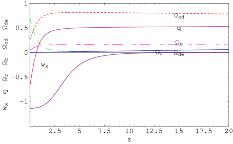
Figure 1: Case I: The evolution of the dimensionless density parameters $\Omega_{cd}$, $\Omega_{de}$, $\Omega_{b}$, $\Omega_{r}$ and deceleration parameter $q$, EOS of dark energy $w_{x}$ versus redshift $z$, where $\Omega_{cd0}=0.25$, $\Omega_{de0}=0.6991$, $\Omega_{b0}=0.05$, $\Omega_{b0}=0.0009$ and $\omega_{0}=-1.14$.

Case II: $w_{\phi}=w_{0}+w_{1}z$ (Ref. [20])

$$\tilde{V}(z) = \frac{1}{2}(1-w_{0}-w_{1}z)(1+z)^{3(1+w_{0}-w_{1})}e^{3w_{1}z},$$ (33)

$$E(z) = (1+z)^{3(1+w_{0}-w_{1})}e^{3w_{1}z},$$ (34)

$$f(z) = (1+z)^{2}\left[\Sigma_{i}\Omega_{\gamma_{i}0}(1+z)^{3(\gamma_{i}+1)}+\Omega_{\phi 0}(1+z)^{3(1+w_{0}-w_{1})}e^{3w_{1}z}\right]^{-1}.$$ (35)

The evolutions of the dimensionless energy density parameters $\Omega_{i}$s, EOS of dark energy $\omega_{x}$ and decelerated parameter $q$ are plotted in Fig. (2) for Case II.

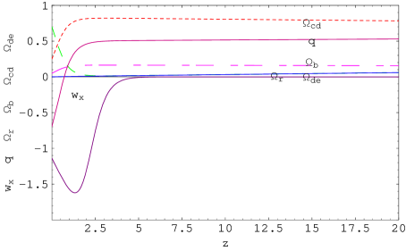
Figure 2: Case II: The evolution of the dimensionless density parameters $\Omega_{cd}$, $\Omega_{de}$, $\Omega_{b}$, $\Omega_{r}$ and deceleration parameter $q$, EOS of dark energy $w_{x}$ versus redshift $z$, where $\Omega_{cd0}=0.25$, $\Omega_{de0}=0.6991$, $\Omega_{b0}=0.05$, $\Omega_{b0}=0.0009$ and $\omega_{0}=-1.14$ and $\omega_{1}=-0.5$.

Case III: $w_{\phi}=w_{0}+w_{1}\frac{z}{1+z}$ (Ref. [21, 22, 23])

$$\tilde{V}(z) = \frac{1}{2}\left(1-w_{0}-w_{1}\frac{z}{1+z}\right)(1+z)^{3(1+w_{0}+w_{1})}e^{-3w_{1}\frac{z}{1+z}},$$ (36)

$$E(z) = (1+z)^{3(1+w_{0}+w_{1})}e^{-3w_{1}\frac{z}{1+z}},$$ (37)

$$f(z) = (1+z)^{2}\left[\Sigma_{i}\Omega_{\gamma_{i}0}(1+z)^{3(\gamma_{i}+1)}+\Omega_{\phi 0}(1+z)^{3(1+w_{0}+w_{1})}e^{-3w_{1}\frac{z}{1+z}}\right]^{-1}.$$ (38)

The evolutions of the dimensionless energy density parameters $\Omega_{i}$s, EOS of dark energy $\omega_{x}$ and decelerated parameter $q$ are plotted in Fig. (3) for Case III.

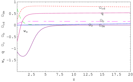
Figure 3: Case III: The evolution of the dimensionless density parameters $\Omega_{cd}$, $\Omega_{de}$, $\Omega_{b}$, $\Omega_{r}$ and deceleration parameter $q$, EOS of dark energy $w_{x}$ versus redshift $z$, where $\Omega_{cd0}=0.25$, $\Omega_{de0}=0.6991$, $\Omega_{b0}=0.05$, $\Omega_{b0}=0.0009$ and $\omega_{0}=-1.14$ and $\omega_{1}=-0.5$.

Case IV: $w_{\phi}=w_{0}+w_{1}\ln(1+z)$ (Ref. [24])

$$\tilde{V}(z) = \frac{1}{2}\left[1-w_{0}-w_{1}\ln(1+z)\right](1+z)^{3(1+w_{0})+\frac{3}{2}w_{1}\ln(1+z)},$$ (39)

$$E(z) = (1+z)^{3(1+w_{0})+\frac{3}{2}w_{1}\ln(1+z)},$$ (40)

$$f(z) = (1+z)^{2}\left[\Sigma_{i}\Omega_{\gamma_{i}0}(1+z)^{3(\gamma_{i}+1)}+\Omega_{\phi 0}(1+z)^{3(1+w_{0})+\frac{3}{2}w_{1}\ln(1+z)}\right]^{-1}.$$ (41)

The evolutions of the dimensionless energy density parameters $\Omega_{i}$s, EOS of dark energy $\omega_{x}$ and decelerated parameter $q$ are plotted in Fig. (4) for Case IV.

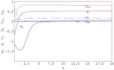
Figure 4: Case IV: The evolution of the dimensionless density parameters $\Omega_{cd}$, $\Omega_{de}$, $\Omega_{b}$, $\Omega_{r}$ and deceleration parameter $q$, EOS of dark energy $w_{x}$ versus redshift $z$, where $\Omega_{cd0}=0.25$, $\Omega_{de0}=0.6991$, $\Omega_{b0}=0.05$, $\Omega_{b0}=0.0009$ and $\omega_{0}=-1.14$ and $\omega_{1}=-0.5$.

From the above examples, it is found that the dark energy dominating the accelerating universe in our case can be obtained by using the correspondence between $f(z)$ and $V(\phi)$. In the above cases, we took the values of parameters at discretion to describe the correspondence. The observation values of the parameters can be determined by the data from supernovae observations easily.

5 Conclusions

A general class of $5D$ cosmological models is characterized by a big bounce as opposed to the big bang in $4D$ standard cosmological model. This exact solution contains two arbitrary functions $\mu(t)$ and $\nu(t)$, which are in analogy to the different forms of the potential $V\left(\phi\right)$ in quintessence or phantom dark energy models. Also, once the forms of the arbitrary functions are specified, the universe evolution will be determined. In this paper, we study these correspondence between the arbitrary function $f(z)$ and the scalar field potential $V(\phi)$. By these correspondences, we can define the arbitrary form $f(z)$. And then the evolution of the universe is determined by the correspondence. Four special cases of potentials $V(\phi)$ are discussed. In all these cases, dark energy dominated accelerating universe are obtained.

6 Acknowledgments

This work was supported by National Natural Science Foundation (10273004) and National Basic Research Program (2003CB716300) of P. R. China.

7 References

References

- [1] A.G. Riess, et.al., Observational evidence from supernovae for an accelerating universe and a cosmological constant, Astron. J. 116 1009 (1998), astro-ph/9805201; S. Perlmutter, et.al., Measurements of omega and lambda from 42 high-redshift supernovae, Astrophys. J. 517 565 (1999), astro-ph/9812133.
- [2] J.L. Tonry, et.al., Cosmological Results from High-z Supernovae , Astrophys. J. 594 1 (2003), astro-ph/0305008; R.A. Knop, et.al., New Constraints on , , and w from an Independent Set of Eleven High-Redshift Supernovae Observed with HST, astro-ph/0309368; B.J. Barris, et.al., 23 High Redshift Supernovae from the IfA Deep Survey: Doubling the SN Sample at z¿0.7, Astrophys.J. 602 571 (2004), astro-ph/0310843.
- [3] A.G. Riess, et.al., Type Ia Supernova Discoveries at From the Hubble Space Telescope: Evidence for Past Deceleration and Constraints on Dark Energy Evolution, astro-ph/0402512.
- [4] P. de Bernardis, et.al., A Flat Universe from High-Resolution Maps of the Cosmic Microwave Background Radiation, Nature 404 955 (2000), astro-ph/0004404; S. Hanany, et.al., MAXIMA-1: A Measurement of the Cosmic Microwave Background Anisotropy on angular scales of 10 arcminutes to 5 degrees, Astrophys. J. 545 L5 (2000), astro-ph/0005123; D.N. Spergel et.al., First Year Wilkinson Microwave Anisotropy Probe (WMAP) Observations: Determination of Cosmological Parameters, Astrophys. J. Supp. 148 175 (2003), astro-ph/0302209.
- [5] I. Zlatev, L. Wang, and P.J. Steinhardt , Quintessence, Cosmic Coincidence, and the Cosmological Constant, Phys. Rev. Lett. 82 896 (1999), astro-ph/9807002; P.J. Steinhardt, L. Wang , I. Zlatev, Cosmological Tracking Solutions, Phys. Rev. D 59 123504 (1999), astro-ph/9812313; M.S. Turner , Making Sense Of The New Cosmology, Int. J. Mod. Phys. A 17S1 180 (2002), astro-ph/0202008; V. Sahni , The Cosmological Constant Problem and Quintessence, Class.Quant.Grav. 19 3435 (2002), astro-ph/0202076.
- [6] R.R. Caldwell, M. Kamionkowski, N.N. Weinberg, Phantom Energy: Dark Energy with w Causes a Cosmic Doomsday, Phys. Rev. Lett. 91 071301 (2003), astro-ph/0302506; R.R. Caldwell, A Phantom Menace? Cosmological consequences of a dark energy component with super-negative equation of state, Phys. Lett. B 545 23 (2002), astro-ph/9908168; P. Singh, M. Sami, N. Dadhich, Cosmological dynamics of a phantom field, Phys. Rev. D 68 023522 (2003), hep-th/0305110; J.G. Hao, X.Z. Li , Attractor Solution of Phantom Field, Phys.Rev. D 67 107303 (2003), gr-qc/0302100.
- [7] V. Sahni, Theoretical models of dark energy, Chaos. Soli. Frac. 16 527 (2003).
- [8] Armendáriz-Picón, T. Damour, V. Mukhanov, k-Inflation, Physics Letters B 458 209 (1999); M. Malquarti, E.J. Copeland , A.R. Liddle, M. Trodden, A new view of k-essence, Phys. Rev. D 67 123503 (2003); T. Chiba , Tracking k-essence, Phys. Rev. D 66 063514 (2002), astro-ph/0206298.
- [9] Z.K. Guo, N. Ohtab and Y.Z. Zhang, Parametrization of Quintessence and Its Potential, astro-ph/0505253.
- [10] T. Kaluza, On The Problem Of Unity In Physics, Sitzungsber. Preuss. Akad. Wiss. Berlin (Math. Phys.) K1 966 (1921).
- [11] O. Klein, Quantum Theory And Five-Dimensional Relativity, Z. Phys. 37 895 (1926) [Surveys High Energ. Phys. 5 (1926) 241].
- [12] J.E. Campbell, A Course of Differential Geometry, (Clarendon Oxford, 1926); S. Rippl, R. Romero, R. Tavakol, Gen. Quantum Grav. 12 2411 (1995); C. Romero, R. Tavako and R. Zalaletdinov, Ge. Relativ. Gravit. 28 365 (1996); J. E.Lidsey, C. Romero, R. Tavakol and S. Rippl, Class. Quantum Grav. 14 865 (1997); S.S. Seahra, P.S. Wesson, Application of the Campbell-Magaard theorem to higher-dimensional physics, Class. Quant. Grav. 20 1321 (2003), gr-qc/0302015.
- [13] P.S. Wesson, Space-Time-Matter (Singapore: World Scientific) 1999; J.M. Overduin and P.S. Wesson, Phys. Rept. 283, 303 (1997), gr-qc/9805018.
- [14] V. Frolov, M. Snajdr, D. Stojkovic, Interaction of a brane with a moving bulk black hole, Phys. Rev. D 68, 044002 (2003).
- [15] H.Y. Liu and P.S. Wesson, Universe models with a variable cosmological “constant” and a “big bounce”, Astrophys. J. 562 1 (2001), gr-qc/0107093.
- [16] T. Liko, P.S. Wesson, The Big Bang as a Phase Transition, Int. J. Mod. Phys. A 20 2037 (2005), gr-qc/0310067; S.S. Seahra, P.S. Wesson, Universes encircling five-dimensional black holes, J. Math. Phys., 44 5664 (2003); Ponce de Leon J, Gen. Relativ. Gravit. 20 539 (1988); L.X. Xu , H.Y. Liu, B.L. Wang, Big Bounce singularity of a simple five-dimensional cosmological model, Chin. Phys. Lett. 20 995 (2003), gr-qc/0304049; H.Y. Liu, Exact global solutions of brane universe and big bounce, Phys. Lett. B 560 149 (2003), hep-th/0206198.
- [17] B.L. Wang, H.Y. Liu, L.X. Xu, Accelerating Universe in a Big Bounce Model, Mod. Phys. Lett. A 19 449 (2004), gr-qc/0304093; L.X. Xu, H.Y. Liu, Three Components Evolution in a Simple Big Bounce Cosmological Model, Int. J. Mod. Phys. D 14 883 (2005), astro-ph/0412241.
- [18] H.Y. Liu and B. Mashhoon, A machian interpretation of the cosmological constant, Ann. Phys. 4 565 (1995).
- [19] S. Hannestad and E. Mortsell, Phys. Rev. D 66 063508 (2002).
- [20] A.R. Cooray and D. Huterer, Astrophys. J. 513 L95 (1999).
- [21] M. Chevallier, D. Polarski, Int. J. Mod. Phys. D 10 213 (2001); gr-qc/0009008.
- [22] E.V. Linder, Phys. Rev. Lett. 90 091301 (2003).
- [23] T. Padmanabhan and T.R. Choudhury, Mon. Not. Roy. Astron. Soc. 344 823 (2003).
- [24] B.F. Gerke and G. Efstathiou, Mon. Not. Roy. Astron. Soc. 335 33 (2002).
- [25] J. Ponce de Leon, Gen. Relativ. Gravit. 20 539 (1988).
- [26] F. Dahia and C. Romero, Dynamically generated embeddings of spacetime, gr-qc0503103.