Testing the ‘dark-energy’-dominated cosmology via the Solar-system experiments

Abstract

The effect of ‘dark energy’ (i.e. the $\Lambda$-term in Einstein equations) is sought for at the interplanetary scales by comparing the rates of secular increase in the lunar orbit obtained by two different ways: (1) measured immediately by the laser ranging and (2) estimated independently from the deceleration of the Earth’s proper rotation. The first quantity involves both the well-known effect of geophysical tides and the Kottler effect of $\Lambda$-term (i.e. a kind of the ‘local’ Hubble expansion), while the second quantity is associated only with the tidal influence. The difference between them, 2.2$\pm$0.3 cm yr^-1, can be attributed just to the local Hubble expansion with rate $H_{0}^{\rm(loc)}\!=56{\pm}8$ km s^-1 Mpc^-1. Assuming that Hubble expansion is formed locally only by the uniformly distributed dark energy ($\Lambda$-term), while globally also by a clumped substance (for the most part, the cold dark matter), the total (large-scale) Hubble constant should be $H_{0}=65{\pm}9$ km s^-1 Mpc^-1. This is in reasonable agreement both with the commonly-accepted WMAP result, $H_{0}=71{\pm}3.5$ km s^-1 Mpc^-1, and with the data on supernovae Ia distribution. The above coincidence can serve as one more argument in favor of the dark energy.

1 Introduction

According to the recent astronomical data, the most part of energy density in the Universe (up to 75%) is in the ‘dark’ form (such as the so-called ‘quintessence’, inflaton potential, polarization of vacuum and so on), which is effectively described by $\Lambda$-term in the Einstein equations (e.g. reviews by van den Bergh, 1999; Chernin, 2001; Krauss, 2004, etc.). All arguments in favor of the dark energy were obtained so far from the observational data related to very large (intergalactic) scales, such as a distribution of supernovae Ia as function of their redshift, the spectrum of fluctuations of the cosmic microwave background radiation, the spectra of absorption lines from distant sources, or Ly$\alpha$ forest, and so on.

Is it possible to find a manifestation of the dark energy at much less scales (e.g. inside the Solar system)? In general, such effects can be expected from the solution of the equations of General Relativity for a point-like mass $M$ in the $\Lambda$-dominated (de Sitter) Universe, which was obtained by Kottler (1918) a very short time after the original Schwarzschild solution. (More details are given in Appendix A.)

The presence of $\Lambda$-term should change, particularly, the standard relativistic shift of Mercury’s perihelion, predicted by General Relativity. This was the idea by Cardona & Tejeiro (1998), who proposed using the measure of the uncertainty in our knowledge of Mercury’s perihelion shift to impose the upper bound on $\Lambda$. The result obtained was not so good as other cosmological estimates but, surprisingly, the accuracy was worse by only $1{\div}2$ orders of magnitude. So, according to the above-cited authors, improvement of the value of the shift by one or two decimal digits should make such method of determination of $\Lambda$ competitive with the observations at large scales. A more skeptical viewpoint on the same subject was presented recently by Iorio (2006).

In any case, since accuracy of the above method is still insufficient, it was proposed in our previous papers (Dumin, 2001, 2003) to utilize the data of radial (rather than angular) measurements of the Moon to reveal anomalous increase in its orbit produced by the $\Lambda$-term in metric (11)–(15), under assumption that the central mass $M$ belongs to the Earth. This looks formally as ‘local’ Hubble expansion. Unfortunately, the result of the earlier works was quite strange: the ‘local’ Hubble constant was found to be approximately in the middle between zero and the standard intergalactic value, which did not allow a reasonable quantitative interpretation.

The aim of the present work is to describe a much improved analysis of the available observations and to show that its results are in reasonable theoretical agreement with the large-scale data.

2 Theoretical viewpoints on the problem of local Hubble expansion

The secular increase in planetary radii due to the $\Lambda$-term, discussed in Appendix A, formally looks like a kind of the Hubble expansion. So, let us briefly discuss why is it necessary to reexamine the problem of local Hubble expansion just in the context of ‘dark-energy’-dominated cosmological models?

In general, Hubble dynamics at the small scales is studied for a long time, starting from the pioneering work by McVittie (1933). Although the results by various authors obtained by now were quite contradictory (e.g. review by Bonnor, 2000, and references therein), the most popular point of view was that the Hubble expansion manifests itself only at the sufficiently large distances (from a few Mpc) and is absent at the less scales at all (e.g. Misner, Thorne & Wheeler, 1973). There were a few arguments in favor of such conclusion.

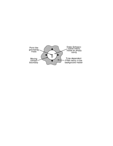
Figure 1: Schematic illustration of the Einstein–Straus theorem.

The first of them is based on the so-called Einstein–Straus theorem (Einstein & Straus, 1945). Let us consider the Friedmann–Robertson–Walker (FRW) cosmological model, uniformly filled with some kind of matter. Next, let us assume that the background matter inside a specified sphere is cut off and concentrated in the point in its centre, as illustrated in Fig. 1. Then, using equations of General Relativity, it can be shown that gravitational field inside the empty cavity is described by the purely static Schwarzschild metric and begins to experience the cosmological expansion only outside its contact boundary with the background matter distribution; this boundary moving just with the Hubble velocity. Therefore, there is no any Hubble expansion in the vicinity of the mass $M$.

Unfortunately, despite a mathematical elegance of this result, it is absolutely unclear how can the above-mentioned cavities be identified for the real astronomical objects. Moreover, this theorem becomes evidently inapplicable at all in the case of ‘dark-energy’-dominated cosmology, because it is meaningless to consider an empty cavity in the vacuum energy distribution.

The second argument against the Hubble expansion at small scales is based on a quasi-Newtonian treatment of Hubble effect in a small volume as a tidal-like action by distant matter (e.g. the recent work by Domínguez & Gaite, 2001, and references therein). The final conclusion usually derived by this way is that there should be no Hubble expansion in the gravitationally-bound systems (i.e. the ones whose kinetic energy is less than potential energy), such as the planetary systems or stars in galaxies. According to this criterion, the Hubble expansion should manifest itself only from $5{\div}10$ Mpc, as was actually observed for a long time.

Unfortunately, the tidal treatment of Hubble effect is not well justified from the theoretical point of view. Besides, more accurate astronomical measurements in the recent few years revealed a well-formed Hubble flow down to the distances of about 1 Mpc, which are considerably less than the scale of gravitational unbinding (Chernin, 2001; Ekholm et al., 2001). Moreover, in the $\Lambda$-dominated cosmology the tidal effects cannot be of primary significance just because of the perfectly uniform distribution of the dark energy and, therefore, may be expected only from minor constituents of the Universe.

At last, one more approach for treating the influence of cosmic expansion on the dynamics of small-scale systems is based on the Einstein–Infeld–Hoffmann (EIH) surface integral method, which enables to derive the equations of motion of the particles immediately from the field equations. This method is based on the integration of field equations over the small closed surfaces surrounding the point-like sources of the field and subsequent use of independence of these integrals on the particular surfaces. Such approach is widely employed to obtain the post-Newtonian equations of motion against the background of flat (Minkowski) space–time and was applied also to the problem of local Hubble expansion by Anderson (1995). It was found that planetary systems should really expand but with a rate much less than for the entire Universe. Unfortunately, the EIH method also becomes inappropriate if the space is filled everywhere with the dark energy, because the surface integrals are no longer invariant when the integration surfaces are moved.

Finally, a frequent experimental argument against Hubble expansion within the Solar system is based on the available constraint on time variation in the gravitational constant derived from the planetary dynamics, which is now as strong as $\,{\dot{G}}/G=\!(4{\pm}9){\times}10^{-13}$ yr^-1 (Williams, Turyshev & Boggs, 2004). So, as was concluded by these authors, “the ${\dot{G}}/G$ uncertainty is 83 times smaller than the inverse age of the Universe, $t_{0}=13.4$ Gyr …  Any isotropic expansion of the Earth’s orbit which conserves angular momentum will mimic the effect of $\dot{G}$ on the Earth’s semimajor axis, ${\dot{a}}/a=-{\dot{G}}/G$ …  There is no evidence for such local (${\sim}1$ AU) scale expansion of the solar system.”

Table 1: Rates of secular increase in the mean Earth–Moon distance.

Method	Immediate measurement by	Independent estimate from the
	the lunar laser ranging	Earth’s tidal deceleration
Effects involved	(1) geophysical tides	(1) geophysical tides
	(2) local Hubble expansion
Numerical value	$3.8{\pm}0.1$ cm yr-1	$1.6{\pm}0.2$ cm yr-1

Unfortunately, the above-stated equivalence between the effect of variable $G$ and the cosmological expansion is based solely on the Newtonian arguments. A more accurate treatment of this problem in the framework of General Relativity for a general case of the multi-component Universe is very difficult. Nevertheless, it can be performed in analytic form for the particular case of a point-like mass in the Universe filled only with dark energy (the $\Lambda$-term), and the corresponding results are outlined in Appendix A. As follows from expressions (16)–(19), the $\Lambda$-dependence of a few terms of the resulting metric tensor can really be reinterpreted as the effect of variable $G$, but this is not true in general: there are some terms whose $\Lambda$-dependence is radically different from any variations in $G$.

3 Analysis of observational data

Since all the commonly-used arguments against the small-scale Hubble expansion fail in the case of dark energy, it becomes reasonable to seek for the corresponding effect; and the most sensitive tool seems to be the lunar laser ranging (LLR) (e.g. Dickey et al., 1994; Nordtvedt, 1999). For example, if we assume that planetary systems experience the Hubble expansion with the same rate as everywhere in the Universe ($60{\div}70$ km s^-1 Mpc^-1), then average radius of the lunar orbit $R$ should increase by approximately 50 cm for the period of 20 years. On the other hand, the accuracy of LLR measurements during the last 20 years was maintained at the level of $2{\div}3$ cm (Dickey et al., 1994); so the perspective of revealing the local Hubble effect looks very good.

The main obstacle that needs to be got around is to exclude the effect of geophysical tides, which also contributes to the secular increase in the Earth–Moon distance. As is known (e.g. Kaula, 1968), because of dissipative effects, the Earth’s tidal bulge, formed by the lunar attraction, is not perfectly aligned in the direction to the Moon but slightly shifted towards the Earth’s proper rotation. Therefore, there is a torque moment, which decreases the proper angular momentum of the Earth and increases the orbital momentum of the Moon. As a result, the average Earth–Moon distance $R$ gradually increases in the course of time.

According to the law of conservation of angular momentum, the secular variation in $R$ is related to the change in the Earth’s diurnal period $T_{\rm E}$ by the simple formula:

$$\dot{R}=k\,{\dot{T}}_{\rm E}\,,$$ (1)

where $k\!=\!1.81{\times}10^{5}$ cm s^-1 (a more detailed discussion can be found, for example, in our previous work, Dumin, 2003). So, if ${\dot{T}}_{\rm E}$ is known from independent astrometric measurements of the Earth’s rotation deceleration with respect to distant objects, then relation (1) can be used to exclude the influence of geophysical tides and, thereby, to reveal a probable presence of local Hubble expansion.

Unfortunately, ${\dot{T}}_{\rm E}$ is not a well-defined quantity: its values derived from the observations in telescopic era and from the various sets of pre-telescopic data appreciably differ from each other (e.g. Stephenson & Morrison, 1984). It is not so important for us now what is the reason for these discrepancies: this may be the systematic errors in the earliest data or, for example, the tectonic processes appreciably changed the Earth’s moment of inertia just before the period of telescopic observations. Since LLR data refer to the last decades, they should be confronted with the most recent values of the Earth’s rotation deceleration. The corresponding telescopic data, starting from the middle of the 17th century, were processed by a few researches; and one of the most detailed compilations was presented recently by Sidorenkov (2002).

Of course, the value of secular trend derived from the quite short time series can suffer from the considerable periodic and quasi-periodic variations in $T_{\rm E}$. So, the main aim of our statistical analysis outlined in Appendix B was to estimate as carefully as possible the ‘mimic’ effect of such variations. Taking into account the corresponding uncertainty, the resulting value can be written as

$${\dot{T}}_{\rm E}\!=\!(8.77{\pm}1.04){\times}10^{-6}~{}{\rm s}{\,}{\rm yr}^{-1}.$$ (2)

The results of the entire analysis of LLR vs. the astrometric data are summarized in Table 1. The excessive rate of increase of the lunar orbit $2.2{\pm}0.3$ cm yr^-1 can be attributed to the local Hubble expansion with rate

$$H_{0}^{\rm(loc)}=56{\pm}8~{}{\rm km{\,}s^{-1}{\,}Mpc^{-1}}.$$ (3)

This value is appreciably greater than in our earlier work (Dumin, 2003), where it was found to be only $33{\pm}5$ km s^-1 Mpc^-1. This was because of using a substantially different rate of the Earth’s deceleration, ${\dot{T}}_{\rm E}\!=\!1.4{\times}10^{-5}$ s yr^-1. The last-mentioned value was obtained for the first time by Stephenson & Morrison (1984), who used the telescopic observations supplemented by a much longer series of medieval Arabian data; and their result was inaccurately cited in a number of subsequent reviews and monographs (e.g. Pertsev, 2000) as derived from the telescopic observations alone.

Finally, it should be mentioned that the basic relation (1) was written under assumption of constant moment of inertia of the Earth, which is a questionable item. For example, over 20 years ago Yoder et al. (1983) found that Earth’s oblateness, commonly characterized by the gravitational harmonic coefficient $J_{2}$, was decreasing. This was interpreted as viscous rebound of the solid Earth from the decrease in load due to the last deglaciation. The observed secular effect ${\dot{J}}_{2}\!=\!-3{\times}10^{-11}$ yr^-1 resulted in the Earth’s spin-up due to decreasing moment of inertia and, thereby, enabled the above-cited authors to get a reasonable agreement between the various sets of data on the Earth’s rotation. Therefore, following this approach, it would be unnecessary to take into consideration any other influences, such as the cosmological Hubble expansion.

Unfortunately, the early results by Yoder et al. (1983) were not confirmed by the most recent studies. For example, as follows from the analysis by Bourda & Capitaine (2004) performed over a sufficiently long time interval (1985–2002), the coefficient $J_{2}$ has a much smaller secular trend but a considerable oscillatory component with a period of two decades. An even more striking disagreement with the earlier data was obtained by Cox & Chao (2002), who found that since 1997 or 1998 the secular trend in $J_{2}$ has approximately the same absolute value as reported by Yoder et al. (1983) but the opposite sign (namely, ${\dot{J}}_{2}\!=\!+2.2{\times}10^{-11}$ yr^-1). Therefore, we can conclude that (1) a considerable disagreement between the LLR and astrometric data still exists and (2) the coefficient $J_{2}$ experiences most probably a quasi-periodic variation with a typical time scale of a few decades. The last-mentioned property justifies usage of formula (1), because the temporal variations in the Earth’s moment of inertia should be averaged out when data on the Earth’s rotation are taken for the period of ${\sim}350$ years.

4 Theoretical interpretation

How can the value (3) be interpreted? It is reasonable to assume that local Hubble expansion is formed only by the uniformly-distributed dark energy ($\Lambda$-term), while the irregularly-distributed (aggregated) forms of matter begin to affect the Hubble flow at the larger distances, thereby increasing its rate up to the standard intergalactic value.

If the universe is spatially flat and filled only with vacuum and a dust-like (‘cold’) matter, with densities $\rho_{{\Lambda}0}$ and $\rho_{{\rm D}0}$ respectively, then

$$H_{0}=\,\sqrt{\frac{8\pi G}{3}}\;\sqrt{\,\rho_{{\Lambda}0}+\rho_{{\rm D}0}}$$ (4)

(e.g. Landau & Lifshitz, 1975). So, if $H_{0}$ is formed locally only by ${\rho}_{{\Lambda}0}$, while globally by both these terms, ${\rho}_{{\Lambda}0}$ and ${\rho}_{{\rm D}0}$ (or, in terms of the relative densities, ${\Omega}_{{\Lambda}0}={\rho}_{{\Lambda}0}/{\rho}_{\rm cr}$ and ${\Omega}_{{\rm D}0}={\rho}_{{\rm D}0}/{\rho}_{\rm cr}$), then

$$\frac{H_{0}^{\rm(loc)}}{H_{0}}={\left[1+\frac{\Omega_{{\rm D}0}}{\Omega_{{\Lambda}0}}\,\right]}^{-1/2}.$$ (5)

At the commonly-accepted values $\Omega_{{\Lambda}0}\!=\!0.75$ and $\Omega_{{\rm D}0}\!=\!0.25$, we get ${H_{0}}/{H_{0}^{\rm(loc)}}\!\approx 1.15$. Therefore,

$$H_{0}=65{\pm}9~{}{\rm km{\,}s^{-1}{\,}Mpc^{-1}}\,,$$ (6)

which is in reasonable agreement both with the well-known WMAP result, $71{\pm}3.5$ km s^-1 Mpc^-1, and with the most recent Hubble diagram for a complete sample of type Ia supernovae (Reindl et al., 2005), whose interpretation requires a slightly reduced value of $H_{0}$.

On the other hand, at the given ratio ${H_{0}^{\rm(loc)}}\!/{H_{0}}$ we have

$$\frac{\Omega_{{\rm D}0}}{\Omega_{{\Lambda}0}}=\,{\bigg{(}\frac{H_{0}}{H_{0}^{\rm(loc)}}\bigg{)}}^{\!\!2}\,-1\;.$$ (7)

So, using the most popular value of the total Hubble constant $H_{0}\!=\!71$ km s^-1 Mpc^-1 and our value of the local Hubble constant $H_{0}^{\rm(loc)}\!=\!56$ km s^-1 Mpc^-1, we get ${\Omega_{{\rm D}0}}/{\Omega_{{\Lambda}0}}\approx 0.6$, i.e. a much less fraction of the dark energy than the commonly-accepted one. Therefore, a slightly reduced value of $H_{0}$ seems to be a preferable option.

5 Conclusions

As follows from the above analysis, the presence $\Lambda$-term can give us a reasonable explanation of the anomalous increase in the lunar orbit, consistent with the large-scale astronomical data. Thereby, this is one more argument in favor of the dark energy.

Besides, if the local Hubble expansion really exists, it should result in profound consequences not only for cosmological evolution but also for the dynamics of planetary systems and other ‘small-scale’ astronomical phenomena, which have to be studied in more detail.

Appendix A A point-like mass in the Lambda-dominated Universe

Solution of the equations of General Relativity for a point-like mass $M$ in the Universe filled only with $\Lambda$-term is

$${\rm d}s^{2}\!\! \!\!\!=\!\! \!-\,{\Bigl{(}1-\frac{2GM}{c^{2}r^{\prime}}-\frac{\Lambda{r^{\prime}}^{2}}{3}\Bigr{)}}\,c^{2}{\rm d}{t^{\prime}}^{2}$$ (8)

$$\!+\,{\Bigl{(}1-\frac{2GM}{c^{2}r^{\prime}}-\frac{\Lambda{r^{\prime}}^{2}}{3}\Bigr{)}}^{\!\!-1}\!{\rm d}{r^{\prime}}^{2}\!$$

$$\!+\>\>{r^{\prime}}^{2}({\rm d}{\theta}^{2}\!+{\sin}^{2}{\theta}\,{\rm d}{\varphi}^{2})$$

(Kottler, 1918), where $G$ is the gravitational constant, and $c$ is the speed of light (for general review, see also Kramer et al., 1980).

After a transformation to the cosmological Robertson–Walker coordinates

$$r^{\prime}=\,a_{0}\,{\exp}\Bigl{(}\frac{\displaystyle ct}{\displaystyle r_{0}}\Bigr{)}\,r\,,$$ (9)

$$t^{\prime}=\,t-\frac{1}{2}\,\frac{\displaystyle r_{0}}{\displaystyle c}\>\>{\ln}\Bigl{[}1-\frac{\displaystyle a_{0}^{2}}{\displaystyle r_{0}^{2}}\>{\exp}\Bigl{(}\frac{\displaystyle 2ct}{\displaystyle r_{0}}\Bigr{)}\>r^{2}\Bigr{]}\,,$$ (10)

metric (8) takes the form

$${\rm d}s^{2}\!\!\! \!\!\!=\!\! \!\!\!g_{tt}\,c^{2}{\rm d}{t}^{2}+\,2\,g_{tr}\,c\,{\rm d}{t}\,{\rm d}{r}+\,g_{rr}\,{\rm d}{r}^{2}$$ (11)

$$\!+ \!\!\!g_{\theta\theta}\,{\rm d}{\theta}^{2}+\,g_{\varphi\varphi}\,{\rm d}{\varphi}^{2}\,,$$

where

$$g_{tt}=\frac{\displaystyle-{\Bigl{(}1-\frac{r_{g}}{r^{\prime}}-\frac{{r^{\prime}}^{2}}{r_{0}^{2}}\Bigr{)}}^{\!\!2}+{\Bigl{(}1-\frac{{r^{\prime}}^{2}}{r_{0}^{2}}\Bigr{)}}^{\!\!2}\frac{{r^{\prime}}^{2}}{r_{0}^{2}}}{\displaystyle{\Bigl{(}1-\frac{r_{g}}{r^{\prime}}-\frac{{r^{\prime}}^{2}}{r_{0}^{2}}\Bigr{)}}{\Bigl{(}1-\frac{{r^{\prime}}^{2}}{r_{0}^{2}}\Bigr{)}}^{\!\!2}}\>\>,$$ (12)

$$g_{tr}=\frac{\displaystyle{\Bigl{(}1-\frac{{r^{\prime}}^{2}}{r_{0}^{2}}\Bigr{)}}^{\!\!2}-{\Bigl{(}1-\frac{r_{g}}{r^{\prime}}-\frac{{r^{\prime}}^{2}}{r_{0}^{2}}\Bigr{)}}^{\!\!2}}{\displaystyle{\Bigl{(}1-\frac{r_{g}}{r^{\prime}}-\frac{{r^{\prime}}^{2}}{r_{0}^{2}}\Bigr{)}}{\Bigl{(}1-\frac{{r^{\prime}}^{2}}{r_{0}^{2}}\Bigr{)}}^{\!\!2}}\;\frac{r^{\prime}}{r_{0}}\,\frac{r^{\prime}}{r}\>\>,$$ (13)

$$g_{rr}=\frac{\displaystyle{\Bigl{(}1-\frac{{r^{\prime}}^{2}}{r_{0}^{2}}\Bigr{)}}^{\!\!2}-{\Bigl{(}1-\frac{r_{g}}{r^{\prime}}-\frac{{r^{\prime}}^{2}}{r_{0}^{2}}\Bigr{)}}^{\!\!2}\frac{{r^{\prime}}^{2}}{r_{0}^{2}}}{\displaystyle{\Bigl{(}1-\frac{r_{g}}{r^{\prime}}-\frac{{r^{\prime}}^{2}}{r_{0}^{2}}\Bigr{)}}{\Bigl{(}1-\frac{{r^{\prime}}^{2}}{r_{0}^{2}}\Bigr{)}}^{\!\!2}}\;\frac{{r^{\prime}}^{2}}{r^{2}}\>\>,$$ (14)

$$g_{\theta\theta}=\,g_{\varphi\varphi}/{\sin}^{2}{\theta}={r^{\prime}}^{2}.$$ (15)

In the above formulas, $r_{g}\!=2GM/c^{2}$, $r_{0}=\sqrt{3/\Lambda}\,$, and $a_{0}$ is the scale factor of FRW Universe.

Taking $a_{0}\!=1$ at $t\!=0$ and keeping only the lowest-order terms of $\,r_{g}$ and $1/r_{0}$, we get

$$g_{tt}\!\approx-\Bigl{[}1-\frac{2GM}{c^{2}r}\Bigl{(}1-\frac{c\sqrt{\Lambda}\,t}{\sqrt{3}}\Bigr{)}\Bigr{]}\,,$$ (16)

$$g_{tr}\!\approx\frac{4\,GM\sqrt{\Lambda}}{\sqrt{3}\,c^{2}}\>\>,$$ (17)

$$g_{rr}\!\approx\Bigl{[}1+\frac{2GM}{c^{2}r}\Bigl{(}1-\frac{c\sqrt{\Lambda}\,t}{\sqrt{3}}\Bigr{)}\Bigr{]}\Bigl{(}1+\frac{2c\sqrt{\Lambda}\,t}{\sqrt{3}}\Bigr{)}\,,$$ (18)

$$g_{\theta\theta}=\,g_{\varphi\varphi}/{\sin}^{2}{\theta}\approx\,r^{2}\Bigl{(}1+\frac{2c\sqrt{\Lambda}\,t}{\sqrt{3}}\Bigr{)}\,.$$ (19)

As is seen from the above expressions, manifestation of the $\Lambda$-term in some components of the metric tensor looks like the influence of variable $G$, if we assume that $G=G_{0}+{\dot{G}}\,t$, where ${\dot{G}}=-c\sqrt{\Lambda}/\sqrt{3}\,$. Unfortunately, such interpretation is not self-consistent: the $\Lambda$-dependence of other components is irreducible to the effect of variable $G$.

Appendix B Statistical analysis of the Earth’s rotation deceleration

It is well known that diurnal period of the Earth $T_{\rm E}$, along with secular increase in the course of time, experiences a wide range of oscillations with (quasi-)periods from annual scale to many decades and, probably, even longer. In fact, just the long-period variations enforced the most of researchers to supplement the available telescopic data on the Earth’s rotation by ancient records of the solar eclipses (whose reliability was, of course, not so good).

On the other hand, as was already mentioned in the main body of the paper, we are interested in using only the data that are as close as possible to the LLR measurements. Of course, in deriving the secular term from the short data series, a special care should be paid to a probable interference from the oscillatory components: if periods of such oscillations are comparable with the length of the series analyzed, they can partially mimic the secular (linear) term and, therefore, produce a substantial error in its final value. So, the basic idea of our analysis was to simulate such mimic effect and to find its maximum contribution to the secular term.

Let the observational data be fitted by the following function:

$$f(t)=f_{0}+f_{1}\,t+\,a\,\sin(2\pi t/T)+\,b\,\cos(2\pi t/T)\,,$$ (20)

where $T$ is the trial period; and $f_{0}$, $f_{1}$, $a$ and $b$ are the unknown regression coefficients. They are determined, as usual, by minimization of the functional

$$\Phi(f_{0},f_{1},a,b,T,N_{\rm b},N_{\rm e})=\sum_{i=N_{\rm b}}^{N_{\rm e}}{\left[f(t_{i})-f_{i}\,\right]}^{2}$$ (21)

with respect to $f_{0}$, $f_{1}$, $a$ and $b$. Here, $i$ is the number of year, $f_{i}$ is the corresponding observed value of $f$; $N_{\rm b}$ and $N_{\rm e}$ are the beginning and end of the analyzed time interval.

The resulting values of $f_{0}$, $f_{1}$, $a$ and $b$ will be, in general, functions of $T$, $N_{\rm b}$ and $N_{\rm e}$. The extent of ‘mimic’ contribution from the periodic components to the secular term $f_{1}$ (i.e. the contribution under the worst conditions) can be characterized by the quantities

$$f_{1}^{\rm(min)}(N_{\rm b},N_{\rm e})=\,\min_{T}f_{1}(T,N_{\rm b},N_{\rm e})\,,$$ (22)

$$f_{1}^{\rm(max)}(N_{\rm b},N_{\rm e})=\,\max_{T}f_{1}(T,N_{\rm b},N_{\rm e})\,;$$ (23)

while $f_{1}^{\rm(lin)}(N_{\rm b},N_{\rm e})$ will denote the value derived with the purely linear regression function (20), when the coefficients $a$ and $b$ were dropped out a priopi.

The second important task is to estimate the effect of truncation of the time series on the resulting value of the secular term. (Since the earliest telescopic data might be not so reliable, it may be reasonable to exclude them from the analysis.) So, we performed a number of calculations with the shorter data series, when $N_{\rm b}$ changed from 1 to 50 (while $N_{\rm e}$ was always the same).

As was already mentioned, the primary observational data $f_{i}$ were taken from the monograph by Sidorenkov (2002). They represent the mean annual variations in the Earth’s angular velocity $f(t)=(\delta{\Omega}_{\rm E}/{\Omega}_{\rm E})\!\times\!10^{10}$ for the years 1656 to 2000.

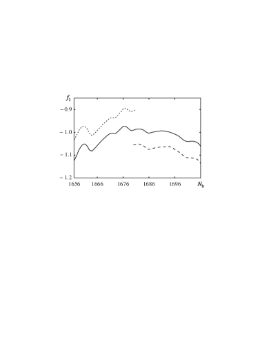
Figure 2: Values of $f_{1}^{\rm(lin)}$ (solid curve), $f_{1}^{\rm(min)}$ (dashed curve) and $f_{1}^{\rm(max)}$ (dotted curve) as functions of the beginning of the data series $N_{\rm b}$. In the intervals where some of the curves are not plotted, the corresponding extrema were not found.

The main results of our regression analysis are shown in Fig. 2. As is seen, the secular term $f_{1}$ can vary in total (as function of both $T$ and $N_{\rm b}$) from $-1.135$ yr^-1 to $-0.895$ yr^-1. So, its average value, distorted by the ‘mimic’ effect of periodic variations and insufficient accuracy of the earliest data, can be written as $f_{1}=-1.015\pm 0.12$ yr^-1. Then, the required rate of the Earth’s diurnal deceleration will be ${\dot{T}}_{\rm E}=-\,T_{\rm E}\,10^{-10}f_{1}$ (where $T_{\rm E}=8.64\!\times\!10^{4}$ s), resulting in ${\dot{T}}_{\rm E}\!=\!(8.77{\pm}1.04){\times}10^{-6}$ s yr^-1.

References

- Anderson (1995) Anderson J.L., 1995, Phys. Rev. Lett., 75, 3602
- Bonnor (2000) Bonnor W.B., 2000, Gen. Rel. Grav., 32, 1005
- Bourda & Capitaine (2004) Bourda G., Capitaine N., 2004, A&A, 428, 691
- Cardona & Tejeiro (1998) Cardona J.F., Tejeiro J.M., 1998, ApJ, 493, 52
- Chernin (2001) Chernin A.D., 2001, Physics–Uspekhi, 44, 1099
- Cox & Chao (2002) Cox C.M., Chao B.F., 2002, Sci, 297, 831
- Dickey et al. (1994) Dickey J.O. et al., 1994, Sci, 265, 482
- Domínguez & Gaite (2001) Domínguez A., Gaite J., 2001, Europhys. Lett., 55, 458
- Dumin (2001) Dumin Yu.V., 2001, Geophys. Res. Abstr., 3, 1965
- Dumin (2003) Dumin Yu.V., 2003, Adv. Space Res., 31, 2461
- Einstein & Straus (1945) Einstein A., Straus E.G., 1945, Rev. Mod. Phys., 17, 120
- Ekholm et al. (2001) Ekholm T., Baryshev Yu., Teerikorpi P., Hanski M.O., Paturel G., 2001, A&A, 368, L17
- Iorio (2006) Iorio L., 2006, Int. J. Mod. Phys. D, 15, 473
- Kaula (1968) Kaula W.M., 1968, An Introduction to Planetary Physics: The Terrestrial Planets. J. Wiley & Sons, NY
- Kottler (1918) Kottler F., 1918, Ann. Phys., 56, 401
- Kramer et al. (1980) Kramer D., Stephani H., MacCallum M., Herlt E., 1980, Exact Solutions of the Einsteins Field Equations. Deutscher Verlag der Wissenschaften, Berlin
- Krauss (2004) Krauss M., 2004, Nat, 431, 519
- McVittie (1933) McVittie G.C., 1933, MNRAS, 93, 325
- Landau & Lifshitz (1975) Landau L.D., Lifshitz E.M., 1975, The Classical Theory of Fields. Pergamon, Oxford
- Misner, Thorne & Wheeler (1973) Misner C.W., Thorne K.S., Wheeler J.A., 1973, Gravitation. W.H. Freeman & Co., San Francisco
- Nordtvedt (1999) Nordtvedt K., 1999, Class. Quant. Grav., 16, A101
- Pertsev (2000) Pertsev B.P., 2000, Izvestiya–Phys. Solid Earth, 36, 218
- Reindl et al. (2005) Reindl B., Tammann G.A., Sandage A., Saha A., 2005, ApJ, 624, 532
- Sidorenkov (2002) Sidorenkov N.S., 2002, Physics of the Earth’s Rotation Instabilities. Nauka-Fizmatlit, Moscow (in Russian)
- Stephenson & Morrison (1984) Stephenson F.R., Morrison L.V., 1984, Phil. Trans. R. Soc. Lond., A313, 47
- van den Bergh (1999) van den Bergh S., 1999, PASP, 111, 657
- Williams, Turyshev & Boggs (2004) Williams J.G., Turyshev S.G., Boggs D.H., 2004, Phys. Rev. Lett., 93, 261101
- Yoder et al. (1983) Yoder C.F., Williams J.G., Dickey J.O., Schutz B.E., Eanes R.J., Tapley B.D., 1983, Nat, 303, 757