Resolving the hard X-ray emission of GX 5-1 with INTEGRAL

We present the study of one year of INTEGRAL data on the neutron star low mass X-ray binary GX 5–1. Thanks to the excellent angular resolution and sensitivity of INTEGRAL, we are able to obtain a high quality spectrum of GX 5–1 from $\sim$5 keV to $\sim$100 keV, for the first time without contamination from the nearby black hole candidate GRS 1758-258 above 20 keV. During our observations, GX 5–1 is mostly found in the horizontal and normal branch of its hardness intensity diagram. A clear hard X-ray emission is observed above $\sim$30 keV which exceeds the exponential cut-off spectrum expected from lower energies. This spectral flattening may have the same origin of the hard components observed in other Z sources as it shares the property of being characteristic to the horizontal branch. The hard excess is explained by introducing Compton up-scattering of soft photons from the neutron star surface due to a thin hot plasma expected in the boundary layer. The spectral changes of GX 5–1 downward along the ”Z” pattern in the hardness intensity diagram can be well described in terms of monotonical decrease of the neutron star surface temperature. This may be a consequence of the gradual expansion of the boundary layer as the mass accretion rate increases.

1 Introduction

Low-mass X-ray binaries (LMXRBs) are systems where the compact object, either a neutron star (NS) or a black hole candidate (BHC), accretes matter from a companion with a mass $\textit{M}\lesssim$ $1\textit{M}_{\odot}$. LMXRBs hosting a weakly magnetised neutron star can be broadly classified in two classes (Hasinger & van der Klis 1989): high luminosity/Z sources and low luminosity/Atoll sources. In the colour-colour (CC) and X-ray hardness intensity diagrams (HID), Atoll sources display an upwardly curved branch while Z sources describe an approximate “Z” shape. Although two recent studies (Muno et al. 2002; Gierliński & Done 2002) have suggested that the clear Z/Atoll distinction on the CC diagram is an artifact due to incomplete sampling (Atoll sources, if observed long enough, do exhibit a Z shape as well) many differences remain. Atoll sources have weaker magnetic fields (about $10^{6}$ to $10^{7}$ G versus 10⁸–10⁹ G of Z sources), are generally fainter ($0.01$–$0.3\,L_{\text{Edd}}$ versus $\sim$$L_{\text{Edd}}$), can exhibit harder spectra and trace out the Z shape on longer time scales than typical Z-sources. Besides, their timing variability properties in a given spectral state are different.

The study of these sources in the hard X-ray domain has proven important especially in the recent years, in the light of the discovery of hard tails extending up to $\sim$100 keV in NS LMXRBs. This kind of hard emission was thought to be a prerogative of BHCs and had been proposed as a possible signature for the presence of a BH (see e.g., McClintock & Remillard 2004). Hard tails discovered in about 20 NS LMXRBs of the Atoll class as well as in some Z sources showed that NS binaries as well can power such an emission (Barret & Vedrenne 1994; Di Salvo & Stella 2002).

GX 5–1 (4U 1758-25) is thought to be a NS LMXRB and is one of the six currently known Galactic Z sources. It displays a complete Z pattern in the CC and HIDs (Kuulkers et al. 1994; Jonker et al. 2002) and shows secular shifts of the ”Z”. As most of the Z sources, it is located near the Galactic Centre which has rendered difficult its study due to source confusion and optical obscuration. Throughout the paper we assumed a distance of 8 kpc and column density N_H = 3$\times$10²² cm^-2 (Asai et al. 1994). Like all Z sources, GX 5–1 is a radio source (e.g. Fender & Hendry 2000) with the radio emission most likely originating in a compact jet. The determination of the radio counterpart allows for extremely accurate position measurements. These have led to a most likely candidate for an infra-red companion (Jonker et al. 2000). In the X-ray domain, up to now neither pulsations nor bursts have been detected (e.g. Vaughan et al. 1994).

Previous GX 5-1 hard X-ray data were almost always contaminated by the nearby (40^′) BHC LMXRB GRS 1758-258. The first mission to clearly resolve GX5-1 from GRS 1758-258 in the high energy domain was GRANAT (Paul et al. 1991). Observations from ART-P ($\sim$5–20 keV), on board GRANAT, showed that GX 5–1 was $\sim$30-50 times brighter than GRS 1758-258 below 20 keV. At higher energies, SIGMA detected only GRS 1758-258 (Sunyaev et al. 1991; Gilfanov et al. 1993).

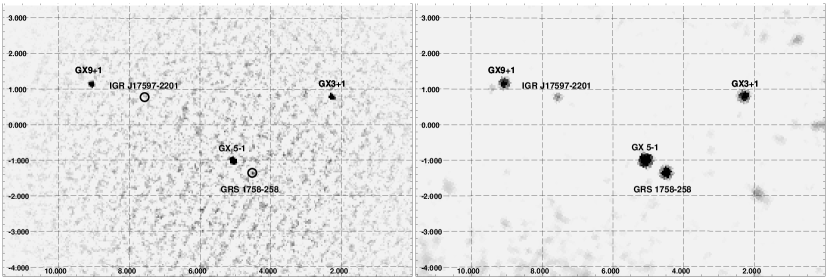
Figure 1: Mosaic images combining the April 2003 and October 2003 data sets. Left panel: JEM–X mosaic image of GX 5–1 in the 5–10 keV band (44 ScWs, $\sim$76 ksec). Right panel: IBIS/ISGRI mosaic image of GX5–1 in the 20–30 keV band (90 ScWs, $\sim$167 ksec). The source IGR J17597$-$2201 has been recently discovered by INTEGRAL (Lutovinov et al. 2003).

Figure 2: IBIS/ISGRI light curves of GX 5–1 in the 20–30 keV for the April 2003 and October 2003 coverage (left and rigth panel, respectively). Each point is one ScW (about 2000 s). Error bars are at 1$\sigma$. The observed countrate corresponds to a variability between about 30 and 130 mCrab. In the softer band (i.e. in JEM–X) the source is much brighter, around 1 Crab.

In this paper we report the results of one year of monitoring of GX 5–1 with the INTErnational Gamma-Ray Astrophysics Laboratory, INTEGRAL (Winkler et al. 2003). INTEGRAL is an ideal mission to study the hard X-ray emission of sources in the crowded Galactic Centre region. INTEGRAL/IBIS (Ubertini et al. 2003) has high sensitivity, about $\sim$10 times better than SIGMA, coupled to imaging capability with 12^′ angular resolution above 20 keV. In addition, two X-ray monitors, JEM–X1 and JEM–X2 (Lund et al. 2003), provide the soft-X ray simultaneous coverage (3–35 keV, 3^′ angular resolution). Effectiveness of INTEGRAL in the study of Galactic bulge bright LMXRBs has been demonstrated in Paizis et al. (2003, 2004) using only initial data.

2 Observations and data analysis

INTEGRAL performed a Galactic Plane Scan (GPS) about every 12 days and Galactic Centre Deep Exposures (GCDEs) according to the Galactic Centre visibility. Among these observation programs, GX 5–1 has been continuously in the INTEGRAL field of view around two distinct periods, April 2003 (INTEGRAL Julian Date IJD$\simeq 1200$, hereafter data set 1, $\sim$90 ksec) and October 2003 (IJD$\simeq 1380$, hereafter data set 2, $\sim$77 ksec).

For the analysis we used the available X-ray monitor, JEM–X2 (hereafter JEM–X), for soft photons (3–35 keV) and the low energy IBIS detector, ISGRI (Lebrun et al. 2003) for harder photons (20–200 keV). We have not used PICsIT, the hard photon IBIS detector (Di Cocco et al. 2003), as its peak sensitivity is above 200 keV, well beyond the 20 keV detection limit given by SIGMA. The spectrometer SPI (Vedrenne et al. 2003) has not been used as the presence of the nearby BH GRS 1758-258 could contaminate the data. The separation of the two sources, 40^′, is below the angular resolution of the instrument, $\sim 2.5^{\circ}$.

JEM–X and IBIS/ISGRI data were reduced using the Off-line Scientific Analysis (OSA) package, OSA 4.0. The description of the algorithms used in the scientific analysis can be found in Westergaard et al. (2003) and Goldwurm et al. (2003) for JEM–X and IBIS/ISGRI respectively. XSPEC 11.3.0 was used for the spectral analysis. The Comptonisation model by Nishimura et al. (1986) (COMPBB) was updated so that the cutoff energy of the model, originally at 70 keV, would suit ISGRI spectra (i.e. moved up to 300 keV).

We used JEM–X to build the hardness intensity diagram (HID) of GX 5–1. This was done using all the JEM–X data available with off-axis angle $<5^{\circ}$ which led to 113 science windows (hereafter ScWs) around 2000 sec exposure each. We extracted individual images from each ScW in 3 energy bands (3–5, 5–12 and 12–20 keV). A mosaicking tool by Chenevez et al. (2004) was used to obtain the final JEM–X mosaic image. Within each ScW we extracted 100 s bin light-curves and used one ScW and 100 s data bins to build the HID. For the spectral fitting of JEM–X data it is preferable to have the source within $3^{\circ}$ off-axis (better vignetting correction and signal-to-noise ratio). This led to 44 JEM–X ScWs. Spectra were grouped so that each new energy bin contained at least 200 counts. Based on Crab calibration results, 3% systematics have been applied between 5 and 22 keV were the spectral analysis has been performed.
In the case of ISGRI we selected the data within the totally coded field of view (FOV, $<$$4.5^{\circ}$, to avoid the partially to totally coded FOV edge), resulting in a total of 90 ScWs (44 of which are in common with JEM–X). We extracted individual ScW images in 10 energy ranges with the boundaries 20, 30, 40, 50, 60, 80, 100, 150, 300, 500 and 1000 keV. The fluxes extracted in each image and energy band were used to build the light-curves of GX 5–1. Images from each ScW were combined in a final mosaic from which an overall ISGRI spectrum was extracted. Spectra were also extracted from each ScW with the Least Square Method and were further grouped so that each new energy bin had a minimum of 20 counts. A 5% systematics has been applied to all channels. For the spectral fitting we used the OSA 4.0 ancillary response file (ARF) and redistribution matrix (RMF) re-binned to 16 spectral channels between 20 and 120 keV.
Simultaneous ISGRI and JEM–X fitting was carried out for the 44 JEM–X ScWs. The remaining 46 ISGRI ScWs were not analysed separately because there was not enough statistics to study ISGRI spectra alone on a ScW basis. In the JEM–X - ISGRI simultaneous fit a cross-calibration factor was let free to vary.

3 Results

3.1 Overview of the data

Figure 1 shows the JEM–X, 5–10 keV, and IBIS/ISGRI, 20–30 keV, mosaic image of the region of GX 5–1 (April 2003 and October 2003 data sets combined). The nearby BHC GRS 1758-258 is rather dim in the softer energy range (JEM–X) and becomes much brighter in the harder range (ISGRI) where it is clearly disentangled from GX 5–1. In the ISGRI mosaic, we detect GX 5–1 with about 4 counts/sec and a detection significance of about 100. In the same image, GRS 1758-258 is detected with an average countrate of about 2 counts/sec and a detection significance of about 50. For comparison, the average count rate obtained from Crab, in different positions of the totally coded field of view, is about 75 counts/sec in the 20–30 keV. In Fig. 2 the overall ISGRI 20–30 keV light curve of GX 5–1 is shown. Each data point corresponds to one ScW in which GX 5–1 has been automatically detected by the software. This happens in 66 ScWs (out of 90) in the 20–30 keV band (with detected countrate between 2 and 10 counts/sec, i.e. between about 30 and 130 mCrab) and in 10 ScWs in the 30–40 keV band (less than 2 counts/sec, $\sim$60 mCrab). In the remaining ScWs, GX 5–1 was not reaching the detection significance of 3, set as a threshold for the automatic detection in a single ScW. The combination of all the ScWs ($\sim$2 ksec each) in a single mosaic (167 ksec, Fig. 1) allows to reveal a hard X-ray emission above $\sim$20 keV.
In the softer energy range covered by JEM–X, GX 5–1 is much brighter (around 1 Crab) and is detected in each 100 sec bin with an average of 27 counts/sec (3–5 keV), 56 counts/sec (5–12 keV) and 5 counts/sec (12–20 keV).

3.2 The hardness intensity diagrams

In order to build the HID of GX 5–1 we used the JEM–X soft colour, defined as the (5–12 keV) to (3–5 keV) flux ratio, plotted versus the JEM–X intensity (defined as the 3–12 keV flux).

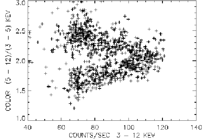
Figure 3: HID of GX5–1 with JEM–X (data set 1). The soft colour is the (5–12 keV) to (3–5 keV) flux ratio. The graph was built using 100 s time bins that were smoothed with a three bin box-car: this means that each 100 s data value is replaced by the mean of the three neighbouring values. The smoothing was chosen for visualisation purposes as it makes the ”Z” more evident. The horizontal branch (upper part, soft colour $>2$) and normal branch (lower part, soft colour $<2$) are clearly visible.

Figure 3 shows the HID we obtained for the first data set (April 2003). The graph was built starting from the 100 s bins that were smoothed to a 5 minute final bin for visualisation purposes. The horizontal branch, HB, and normal branch, NB, are quite evident while the flaring branch, FB, the last part of the ”Z”, is not visible. The FB could be hidden in the data since in GX 5–1 it is short and/or spread out by our choice of energy boundaries. Note the similarity with the HID derived from GINGA/ASM data (van der Klis et al. 1991) and Mir/Kvant TTM data (Blom et al. 1993).

Figure 4 shows the ”raw”, i.e. non-smoothed, HIDs obtained for the two data sets (April 2003 and October 2003 respectively). In the first data set the HB-NB vertex was set to (118,2.15) judging from the overall distribution of the data points. Then the slopes of the ”Z” were calculated so that an equal number of data points were left on either side of the line. The deduced slopes are shown in Fig. 4 with a solid line. As the first data set has a cleaner ”Z” pattern, we used this one as the ”true” one to which the second ”Z” was forced to bend. This was done shifting the HB-NB vertex of the second data set until the slopes of HB and NB became equal to those of the first data set. This led to a vertex in the second set at (115.1, 2.4) which resulted in a clear secular shift from 2.15 to 2.4 in the soft colour of the vertex. Since the current data have an almost continuous coverage from the HB through the NB while coverage of the FB (if any) is very poor, in this paper we focus on the HB and NB.

Figure 4: HID of GX5–1 with JEM–X for the two data sets. The scattered data points are 100 s bins while the points with error bars are one ScW bins. The average statistical error of the 100 s bins is shown in the bottom right of the graphs. The ScW bin values are computed as average of 100 s bins and the associated error is not the statistical one but a measure of how much the source moved along the ”Z” track within the ScW. The solid line shows the deduced ”Z” for the two data sets. Left panel: data set 1 (April 2003). Right panel: data set 2 (October 2003). The ”Z” shape is less evident in this data set with respect to the left panel. This change could be intrinsic to the source as the exposure time in the two data sets is comparable (58 ScWs in data set 1 and 55 ScWs in data set 2).

In order to investigate the correlation between the source position in the ”Z” pattern of the HID and the spectral behaviour, we introduced a one dimensional parameter that measures the position on the ”Z”: S_Z (Dieters & van der Klis 2000, and references therein). Strong evidence shows that the mass accretion rate $\dot{\textit{M}}$ of individual Z sources increases from the top-left to the bottom-right of the ”Z” pattern (Hasinger et al. 1990), i.e. along the HB, NB and FB. Hence, the S_Z parameter is supposed to be monotonically related to the mass accretion rate.

For each JEM–X data point (100 s bin and one ScW bin) in the HIDs, the two projections onto both branches and the distance to each branch were computed. The branch at the shortest distance was chosen and after confirmation via visual inspection, to ensure that data points did not jump from branch to branch outside the vertex area, the value of S_Z was assigned. The scale was set so that the HB-NB vertex was at S${}_{Z}=1$ while S${}_{Z}=0$ and S${}_{Z}=2$ were assigned at a 3–12 keV intensity of 40 counts/s (beginning of HB and end of NB respectively). In this frame, S_Z$<$1 means the source is on the HB (lower $\dot{\textit{M}}$) and 1$<$S_Z$<$2 means that the source is on the NB (higher $\dot{\textit{M}}$).

3.3 Energy Spectral Modeling

We averaged all the ISGRI and JEM–X data to achieve the best statistics and tried to find the most physically reasonable spectral model to fit the entire data set. The ISGRI (average) spectrum was obtained from the mosaic image shown in Fig. 1, right panel, and the JEM–X total spectrum by averaging the 44 JEM–X ScW spectra. In this case, the JEM-X spectrum was further grouped to have a number of energy bins comparable to ISGRI.

The X-ray spectra of bright LMXRBs hosting a NS are generally described as the sum of a soft and a hard component. Two different models are often adopted to describe this composite emission. They are the so-called eastern model (Mitsuda et al. 1984) and western model (White et al. 1986).

In the eastern model the softer part of the spectrum is a multi-colour disc describing the emission from the optically-thick, geometrically-thin accretion disc (XSPEC DISKBB model, Mitsuda et al. 1984). The temperature at the inner disc radius kT_in and the normalisation, linked to the inner disc radius itself, are the parameters of the model. The harder part of the spectrum is a higher temperature Comptonised blackbody describing the emission from the NS boundary layer (COMPBB model, Nishimura et al. 1986). Photons from the NS surface at a temperature kT_bb are up-scattered by a plasma of temperature kT_e and optical depth $\tau$. In this case the normalisation is linked to the seed photon emitting area.

In the western model a single temperature blackbody (from the optically thick boundary layer) describes the soft part of the spectrum (BB model in XSPEC). Comptonisation of soft seed photons (kT₀) in the innermost region of the accretion disc by a corona of given temperature kT_e and optical depth $\tau$ describes the hard part (Titarchuk 1994, e.g. COMPTT model).

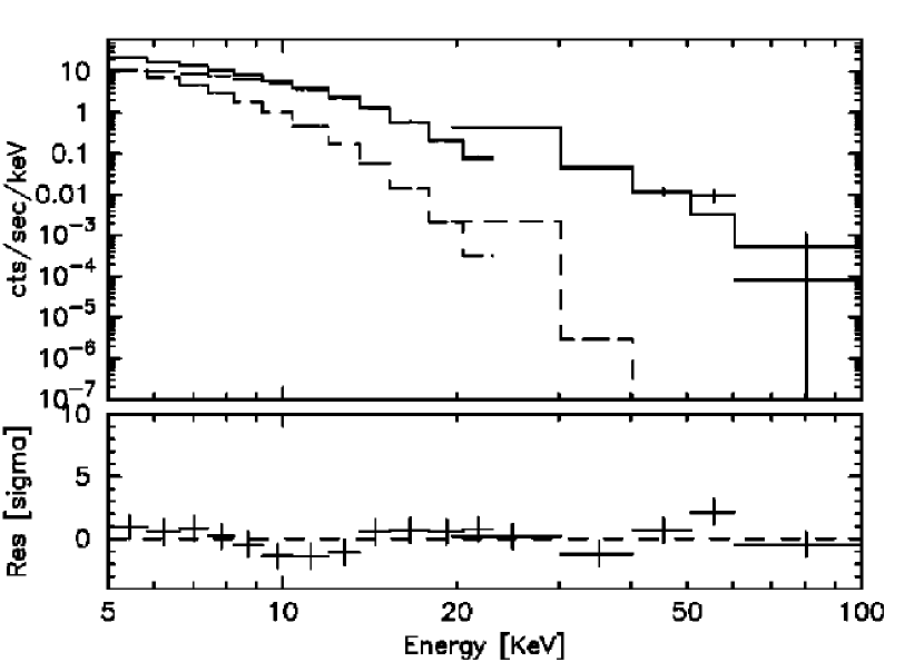
Figure 5: Best fit of the average ISGRI and JEM–X spectra using the eastern model. The parameters of the fit are given in Table 1. Residuals in terms of $\sigma$ and the single spectral components are shown.

Figure 6: Best fit of the average ISGRI and JEM–X spectra using the western model. Residuals in terms of $\sigma$ and the single spectral components are shown. A hard excess above $\sim$30 keV is visible. The parameters of the fit are given in Table 1.

We used the eastern and western model to fit the average JEM–X and ISGRI spectra simultaneously, and compared the results. In both cases a galactic absorption by a fixed hydrogen equivalent column density of N_H = 3$\times$10²² cm^-2 (Asai et al. 1994) was added.

Table 1: Best fit parameters for the average ISGRI and JEM–X spectra of GX 5–1. F${}_{5-20\,\mathrm{keV}}$ and F${}_{20-100\,\mathrm{keV}}$ are the unabsorbed fluxes in the 5-20 keV and 20-100 keV range respectively, in units of  erg s^-1 cm^-2; d.o.f. = degrees of freedom. The indicated errors are at 1$\sigma$. No error means the parameter was fixed to the indicated value. The cross-calibration factor was frozen to 0.9 for ISGRI with respect to JEM-X.

	Eastern model	Western model
kTin or kT (keV)	$1.4$	$1.7$
DISKBB or BB norm	288	0.1
kTbb or kT0	$1.93$$\pm 0.01$ keV	$0.87$$\pm 0.02$ keV
kTe	$10$ keV	$3.02$$\pm 0.02$ keV
$\tau$	$0.37$$\pm 0.01$	$4.15$$\pm 0.06$ keV
COMPBB/COMPTT norm	136	1.6
Red. $\chi$2	$1.12$ ($14$ d.o.f.)	$6.21$($13$ d.o.f.)
F${}_{5-20\,\mathrm{keV}}$	$1.54$$\times$10-8	$1.54$$\times$10-8
F${}_{20-100\,\mathrm{keV}}$	$3.41$$\times$10-10	$3.10$$\times$10-10

The results of the fit are given in Table 1 and Fig. 5 and  6.

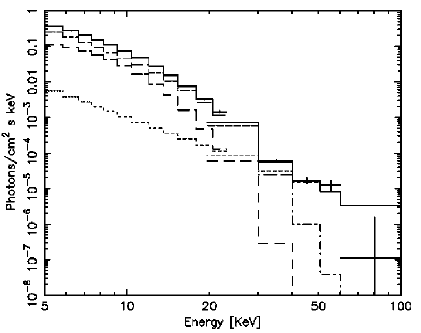
Figure 7: Photon spectrum of GX 5–1 obtained with the western plus additional power-law ($\Gamma$=2.5) model (Red. $\chi$²=1.2, 12 d.o.f.). Dash: NS boundary layer emission (BB). Dot-dash: Comptonisation of innermost region of the accretion disc (COMPTT). Dot: additional power-law. Solid: total spectrum.

Figure 8: Photon spectrum of GX 5–1 obtained with the eastern model described in Table 1. Dash: soft, disc blackbody component. Dot-dash: hard, NS surface blackbody component without Comptonisation ($\tau$=0). A hard excess is evident. Dot (basically overlapping with the solid line): NS blackbody component to which Comptonisation from a 10 keV, $\tau$=0.37 plasma was added. Solid: total spectrum (disc component and NS Comptonised component). The latter two are basically overlapping above 10 keV i.e. almost all the emission is coming from Comptonisation of the NS surface photons.

Both models can describe the spectral shape below $\sim$30 keV equally well. However, in the western model, there is a significant residual in the ISGRI data above $\sim$30 keV, that is reasonably well described in the eastern model. This is because the western model predicts an exponential cut-off above $\sim$10 keV, while the eastern model describes the spectral “flattening” above $\sim$20 keV as a Comptonised hard-tail emission. We are not able to constrain the Comptonising plasma temperature (and consequently the cut-off energy) from our average spectrum. In the eastern model, a good fit can be obtained with a plasma temperature up to about 50 keV. Either the cut-off is above the fitted energy range or our data are not of high enough quality to constrain the spectral break. We choose to fix the temperature to 10 keV as in this frame we can explain in a coherent way the spectral evolution of GX 5–1 (see below).

Adding a power-law component with fixed photon index $\Gamma$$=$$2.5$ in the western model results in a good fit of the observed hard-excess as shown in Fig. 7. In the 5–100 keV band the power-law component alone contributes to about 1.5% of the total luminosity.

Figure 8 shows the photon spectrum obtained with the eastern model parameters shown in Table 1. Since the eastern model provides a physical interpretation for the hard tail, we focus on this model for the analysis and discussion of the spectral changes of GX 5–1.

3.4 Spectral variability along the ”Z”

We studied the spectral variation of GX 5–1 along the HID using the $S_{Z}$ parameter within the frame of the eastern model (with one ISGRI - JEM–X combined spectrum per ScW for a total of 44 ScWs). The soft component (DISKBB) was frozen to the values obtained in the best fit given in Table 1, for all the ScWs. Similarly, the plasma temperature kT_e was fixed at a value of 10 keV, since this parameter is strongly correlated with $\tau$. The normalisation of the hard component, kT_bb and $\tau$ were let free to vary from one Scw fit to the next as well as the instrument cross-calibration factor. An average value of reduced $\chi$²$\simeq$1.2 was obtained. We found a clear relation between the S_Z value and the deduced kT_bb for all the ScWs. To see if we could describe the spectral evolution of GX 5–1 in a more constraining way, we proceeded fitting the data letting in one case kT_bb vary (with $\tau$ fixed to 0.4) and in the other $\tau$ vary (kT_bb fixed to 2.0 keV). In both cases the normalisation was let free as well. Fixing kT_bb resulted in a much worse fit (average reduced $\chi$²$\simeq$2.5) while fixing $\tau$ gave an equally acceptable fit (average reduced $\chi$²$\simeq$1.3). This is consistent with the fact that kT_bb has a clear relation with the position of GX 5–1 along the ”Z” and should not be frozen. Conversely, $\tau$ shows a random distribution of values around 0.4 (extreme cases being 0.1 and 0.8), it is not the main parameter driving the spectral evolution along the ”Z” and hence can be fixed.
The combined JEM–X and ISGRI spectral fitting for two ScWs, one for the HB and the other one for the NB, are shown in Fig. 9, left and right respectively. The spectrum extracted from the HB is significantly harder than the NB one. This is true also for the other spectra and the hard X-ray emission is indeed characteristic of the HB. In fact we obtain that the hard X-ray emission (ISGRI countrate) is systematically linked to the position of the source in the CC diagram: Fig. 10 shows the correlation among ISGRI 20–40 keV flux and JEM–X soft colour for the two datasets (off-axis angle $<$$5^{\circ}$). The different symbols used refer to the position of the source in the ”Z” track: the cases that have been identified with the HB have a higher ISGRI flux whereas the NB cases have a lower ISGRI flux. The second dataset, Fig. 10 right panel, has more uncertain cases as expected given that its ”Z” shape is less clean than for the first dataset.

Figure 9: ISGRI and JEM–X spectra for GX 5–1 in two different ScWs. The best fit and residuals in terms of $\sigma$ are shown. The two components of the model (DISKBB and COMPBB) are also shown (dashed lines). The Comptonising component is frozen to kT_e=10 keV and $\tau$=0.4. Left panel: ScW 012000950010 (IJD=1377.57, UTC=2003-10-09). For this ScW S_Z=0.50, i.e. GX 5–1 is in the HB. kT_bb=2.35 keV, red. $\chi$²=1.4 (112 d.o.f.). (The residuals obtained in the two ISGRI bins between 20–30 keV are not significant as they are due to known ISGRI systematics). Right panel: ScW 012200110010 (IJD=1381.63, UTC=2003-10-13). S_Z=1.56 i.e. GX 5–1 is in the NB. The spectrum is softer, only one ISGRI ($>20$ keV) data point met the requirement of a minimum of 20 counts per bin. kT_bb=1.49 keV, red. $\chi$²=1.5 (89 d.o.f.)

Figure 10: Correlation among ISGRI 20–40 keV flux and JEM–X soft colour, intensity ratio (5–12 keV)/(3–5 keV), for the two datasets (April 2003 on the left and October 2003 on the right). Each point is one ScW. The different symbols used refer to the position of the source in the ”Z” track: $\Box$ = clearly HB, $\Diamond$ = uncertain HB, $\triangle$ = HB or NB, $\times$ = clearly NB, $\ast$ = uncertain NB, $+$ = NB or FB. The big boxes indicate transitions between HB and NB (vertex S = 1). The two outliers in the left panel (assigned HB with low ISGRI intensity) are possibly due to systematics.

Figure 11 shows the variation of the emitting hot NS surface area and temperature, kT_bb, along the ”Z” (left and right panel respectively). While GX 5–1 moves from the HB to the NB (left to right in Fig. 11), the size of the emitting surface increases while its temperature decreases.

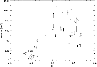
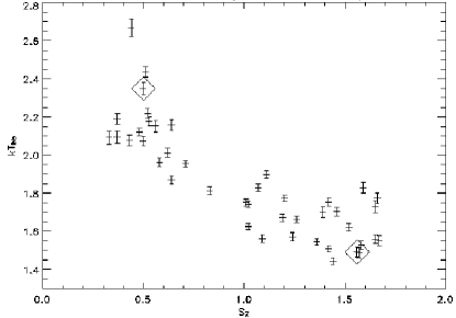
Figure 11: Relations among the seed photons’ properties and position of the source in the ”Z”. The electron plasma temperature kT_e and the optical depth were frozen to 10 keV and 0.4 respectively. In both panels the two ScWs of Fig. 9 are highlighted. Left panel: relation between the blackbody emitting surface and S_Z. The surface is in units of km² and is computed as $\pi$$\times$$d$²$\times$normalisation, where $d$ is the distance of the source in units of 10 kpc, assumed to be 0.8. Right panel: relation between the derived blackbody temperature kT_bb and S_Z.

4 Discussion

Our observations constitute the first opportunity in which the Z source GX 5–1 could be monitored in a long term period in the hard X-ray domain without contamination from the nearby BHC GRS 1758-258.
The source was thoroughly covered by INTEGRAL mainly during two periods (April and October 2003). The HIDs of GX 5–1 for the two periods show a clear secular shift. This is consistent with previous observations of GX 5–1 itself as well as of other Z sources (Kuulkers et al. 1994; Kuulkers & van der Klis 1995, and references therein) for which a secular shift was detected. In our data, GX 5–1 covers widely the HB and NB while very poor coverage of the FB (if any) is seen, similarly to previous observations (e.g., Kuulkers et al. 1994).

4.1 Hard X-ray Emission

The ISGRI and JEM–X average spectra show that GX 5–1 has a clear hard X-ray emission above 20 keV. Assuming a distance of GX 5–1 of 8 kpc, we obtain luminosities of the order of L${}_{1-20\,\mathrm{keV}}$$\sim$10³⁸ erg s^-1 () and L${}_{20-200\,\mathrm{keV}}$$\sim$10³⁶ erg s^-1, fully consistent with values obtained for other Z sources (Di Salvo & Stella 2002). With such luminosities, similarly to the case of the Z sources GX 17+2 and GX 349+2, GX 5-1 lies outside the so-called burster box (Barret et al. 2000), in a region that was originally believed to be populated by BH LMXRBs. Like BHs, NS LMXRBs can have a hard X-ray emission when they are bright.

At least in the cases in which a cut-off is observed, the hard X-ray emission can be interpreted as thermal Comptonisation of soft photons in a hot, optically thin plasma in the vicinity of the neutron star. In the case of GX 5–1 we are not able to constrain the Comptonising plasma temperature. This suggests that either our data are not of good enough quality to measure the cut-off or that the cut-off is beyond the fitted energy range. In any case, we do obtain a good fit with relatively low plasma temperatures (10 keV) hence non-thermal processes, even if not ruled out, cannot be claimed.

In cases where the cut-off has not been observed up to about 100 keV or higher (Di Salvo et al. 2000, 2001), extremely high electron temperatures are required, which is unlikely, given that the bulk of the emission of Z sources is very soft. Non attenuated power-law tails dominating the spectra at high energies may be produced by mildly relativistic ($v/c\sim 0.1$) outflows with flatter power laws corresponding to higher optical depth of the scattering medium and/or higher bulk electrons velocities, in a way that is similar to thermal Comptonisation (Psaltis 2001). Alternatively, X-ray components could originate from the Comptonisation of seed photons by the non thermal high energy-electrons of a jet (Di Salvo & Stella 2002, and references therein) or via synchrotron self-Compton emission directly by the jet (Markoff & Nowak 2004).

4.2 Spectral Variation

With INTEGRAL, we are able to study the spectral state of GX 5–1 within one ScW seeing the source variability above 20 keV that has never been studied before. On the other hand, the softer part of the spectrum, dominated by the disc emission, cannot be constrained and thus we fixed it to the value found from the JEM-X average spectrum.

The spectral changes of GX 5–1 along the ”Z” can be explained by the smooth variation of the physical properties of the seed photons originating from the hot NS surface (heated by the boundary layer). This scenario is different from the more complicated ones that e.g. Hasinger et al. (1990) and Hoshi & Mitsuda (1991) proposed to explain GINGA data of Cyg X–2 and GX 5–1 respectively. Hasinger et al. (1990) studied the spectral variations of Cyg X-2 using both the eastern and western model. The temperature and the luminosity of both components (soft and hard) were let free to vary in both models and a rather complicate interplay of the parameters of both components was describing the spectral variations of the source along the ”Z” pattern. Hoshi & Mitsuda (1991) used the eastern model for GX 5–1 and the spectral changes were also in this case due to the variation of different parameters: in the NB the inner disc radius temperature kT_in and the NS boundary layer temperature kT_bb remained constant and spectral shape changes were explained by an increase of the emission area (from lower left to upper right NB). While the spectrum became harder, in the HB, an additional parameter, kT_in, was let free to reproduce the trend of the data.

Unlike GINGA, with INTEGRAL data we cannot constrain the variability of the disc component and thus we had to fix it to the values found from the average spectra. The normalisation of this component (modelled with DISKBB in XSPEC terminology) led to an inner disc radius of R_in(cos$\theta$)^1/2 $\simeq$14(cos$\theta$)^1/2 km for an assumed source distance of 8 kpc where $\theta$ is the angle between the normal to the disc and the line of sight. In the inner region of the disc, a hot outer layer affects the emergent spectra by Comptonisation. This leads to an observed temperature T_col which is higher than the effective temperature T_eff. As a consequence the observed inner disc radius is underestimated by a factor of (T_col/T_eff)². With this hardening factor correction assumed to be 1.5 (Ebisawa et al. 1991), we obtained an inner disc of about R_eff(cos$\theta$)^1/2$\simeq$30(cos$\theta$)^1/2 km.

Not being sensitive to changes in the softer part of the spectrum is a limitation in our study as we do expect the soft part of the spectrum (the disc) to vary but, for the first time, we were able to study the variability of GX 5–1 in the less explored hard X-rays, above 20 keV. We see that the hard component is indeed chatacteristic of the HB, namely the spectrum is harder at lower accretion rates. This seems to be the general trend in LMXRBs (Barret & Vedrenne 1994). Atoll sources are thought to be at a lower level of accreting rate than Z sources and indeed they are generally harder. This trend continues also within a class of sources: the hard components observed in the Z sources GX 17+2 (Di Salvo et al. 2000), Cyg X-2 (Di Salvo et al. 2002) and GX349+2 (Di Salvo et al. 2001) decrease in intensity from HB to NB and FB, i.e. for increasing mass accretion rate. An exception to this trend was found in Sco X–1 (D’Amico et al. 2001) where the presence of the hard component was not related to the position of the source in the ”Z” track. Theoretical interpretations for this general trend have already been discussed (Inogamov & Sunyaev 1999; Popham & Sunyaev 2001; Kluzniak & Wagoner 1985).

Popham & Sunyaev (2001) have computed the boundary layer structure and its evolution with mass accretion rate $\dot{\textit{M}}$. They found a significant dependence of the boundary layer size (both height and radial extension) with $\dot{\textit{M}}$. Matter falls on a portion of the NS surface that is touched by the boundary layer. This part of the NS surface is thermalised and emits blackbody emission. As $\dot{\textit{M}}$ increases, the area covered by the boundary layer will increase and so will the NS surface responsible of the blackbody emission. This is the same trend we found in the case of GX 5–1 (Fig. 11, left): S_Z, i.e. $\dot{\textit{M}}$, increases and the emitting NS surface increases. This trend is more clearly visible in the HB than in the NB. A possible explanation for this could be that along the NB (with increasing mass accretion rate), the accretion disc, i.e. the soft part of the spectrum that we are not able to constrain with INTEGRAL, is starting to change. Besides, in the NB $\dot{\textit{M}}$ is not expected to vary much (as it is already close to $\dot{\textit{M}}_{Edd}$) so this may be also (part of) the reason why there is no clear trend in the NB.

The 5–100 keV observed luminosity reached a maximum variation of a factor of $\sim$3, unabsorbed L${}_{5-100\,\mathrm{keV}}$$\simeq$(0.6-1.7)$\times$10³⁸ erg s^-1 (). This is small compared to the NS emitting surface variation (factor of $\sim$20, see Fig. 11 left). L${}_{5-100\,\mathrm{keV}}$ is the total luminosity obtained from the composition of soft and hard component between 5–100 keV but the variation in L${}_{5-100\,\mathrm{keV}}$ is to be attributed to the changes in the hot NS surface properties alone as the boundary layer dominates the emission and the disc as well as the parameters of the Comptonising plasma were kept fixed. In our interpretation, any variation in L${}_{5-100\,\mathrm{keV}}$ is a consequence of changes in the properties of the hot NS surface that we modelled with a blackbody emission. Its luminosity is proportional to the emitting surface and temperature, L_bb $\propto$R²$\times$T_bb⁴. So, if the luminosity stays nearly constant (factor of $\sim$3) while the emitting surface increases (factor of $\sim$20), then the temperature of the emitting surface will decrease. Thus, the anti-correlation that we found between S_Z and the blackbody temperature kT_bb (Fig. 11, right) may be qualitatively understood.

5 Conclusions

We have studied the X-ray emission of the Z source GX 5–1 with INTEGRAL. A clear hard emission above $\sim$20 keV is detected and it may have the same origin of the hard components observed in other Z sources as it shares the property of being characteristic to the HB. We used the so-called “eastern” and “western” model to fit the average spectra of GX 5–1. The eastern model describes the spectral “flattening” above $\sim$20 keV as a Comptonised hard-tail emission whereas the western one predicts an exponential cut-off above $\sim$10 keV and an additional power-law is needed to account for the hard X-ray emission. Since the eastern model provides a physical interpretation for the hard tail, we focussed on this model for the analysis of the spectral changes of GX 5–1.

We interpret the spectral changes of GX 5–1 along the ”Z” pattern in the hardness intensity diagram in terms of Comptonisation of varying soft photons ($\sim$2 keV) by a hot plasma (10 keV). The soft photons are interpreted as blackbody emission from the part of the NS surface that is heated by the boundary layer. The Comptonising plasma is the boundary layer optically thin plasma. When GX 5–1 moves downwards in the ”Z”, the temperature and optical depth of the Comptonising plasma are not seen to change in the data. What changes along the ”Z” is the temperature of the optically thick emission from the hot NS surface that shows a steady decrease with increasing mass accretion rate. This may be a consequence of the gradual expansion of the boundary layer that we detect in the data. This trend is in agreement with theoretical studies (Popham & Sunyaev 2001) that indeed predict the expansion of the boundary layer surface with increasing mass accretion rate.

With the INTEGRAL long term monitoring we will also have higher chances to catch GX 5–1 in the FB. The behaviour of Z sources on the FB, believed to correspond to super-Eddington accretion, is quite complex and it will be interesting to see if it can be smoothly included in the HB and NB scenario described here. Furthermore we will search for hard tails extending above 100 keV, in GX 5–1 as well as in the other Z sources and NS binaries of our monitoring program.

The synergy of a long term monitoring and a multi-wavelength study should be the best way to understand the physics of hard-X ray emission of LMXRBs. Our collaboration is moving in this direction: regular coordinated INTEGRAL-RXTE observations of a sample of Atoll and Z sources (including GX 5–1) are being performed and simultaneous radio and optical observations are attempted.